Total Potential Optimization Using Metaheuristic Algorithms for Solving Nonlinear Plane Strain Systems

Abstract

Total Potential Optimization using Metaheuristic Algorithms (TPO/MA) is an alternative tool for the analysis of structures. It is shown that this emerging method is advantageous in solving nonlinear problems like trusses, tensegrity structures, cable networks, and plane stress systems. In the present study, TPO/MA, which does not need any specific implementation for nonlinearity, is demonstrated to be successfully applied to the analysis of plane strain structures. A numerical investigation is performed using nine different metaheuristic algorithms and an adaptive harmony search in linear analysis of a structural mechanics problem having 8 free nodes defined as design variables in the minimization problem of total potential energy. For nonlinear stress-strain relation cases, two structural mechanics problems, one being a thick-walled pipe and the other being a cantilever retaining wall, are analyzed by employing adaptive harmony search, which was found to be the best one in linear analyses. The nonlinear stress-strain relations considered in these analyses are hypothetical ones due to the lack of any such relationship in the literature. The results have shown that TPO/MA can solve nonlinear plane strain problems that can be encountered as engineering problems in structural mechanics.

1. Introduction

Finite Element Method (FEM) is a well-known mechanical and structural analysis tool that is used commonly by structural engineers. In FEM applications, firstly matrix equations are prepared for each element, and then these equations are combined to yield a general matrix equation of the form Kx = p where K is the square matrix called stiffness matrix, x is the vector of displacements and p is the vector of loads. This operation can be performed easily for linear and well-constrained systems. For nonlinear systems, either geometrically or materially, K is a function of displacements and loads. It cannot be written as independent of the values in x and p. FEM applications can be used for nonlinear systems, but an iterative procedure is needed. As a negative point to FEM, one can cite the problems that are under-constrained. For these problems K becomes ill-conditioned making the solution impossible. There are several other problems where FEM becomes very difficult to apply, like the cases where the solution is not unique or where there are unilateral or nonlinear constraints [1,2,3,4,5].

An alternative way for the structural analyses is based on calculating the total potential energy of the elements instead of solving their equilibrium equations. Then by combining all these energies by only summing all of them, it is possible to obtain a function of the whole system as a function of x and p. By following the minimization of that function concerning x, the well-known minimum potential energy theorem in mechanics is provided. This approach, called Total Potential Optimization using Metaheuristic Algorithms (TPO/MA) is first applied successfully to analyses of trusses where the optimization part is conducted using different kinds of metaheuristic algorithms. This approach is followed by further applications, with metaheuristic algorithms and hybrid ones, on planar or space trusses [6,7,8], tensegrity structures [9], and cable systems [10,11]. Latest applications concern plane stress problems, with well-known linear constitutive equations [12], or with hypothetical linear constitutive equations [13]. TPO/MA has advantages on special and nonlinear systems. TPO/MA uses iterative search like an optimization problem for both linear and nonlinear systems, while FEM is a direct solution method for linear systems, and also an iterative system for nonlinear ones.

In this study, the main purpose is to add a new type of structure to the existing application area of TPO/MA, namely, plane strain type plates. It is also aimed to show that systems with nonlinear stress-strain relations can be analyzed with this method with the same ease as with systems with linear stress-strain relations. For this purpose, besides linear systems, nonlinear systems are analyzed too. In these applications nonlinear stress-strain relations are hypothetical ones created by the authors, being not aware of any such real relations in the literature. The literature survey conducted has shown that no such nonlinear relations exist in two-dimensional structures, while they are numerous in the one-dimensional case. The nonlinear two-dimensional relations used in this study are of three different types. To find the best suitable metaheuristic method, 10 metaheuristic methods, one of them being the adaptive harmony search (AHS), are applied on a linear case of the first example. The results on these applications have shown that AHS is the one giving the best solution, in the shortest time. Then, the nonlinear cases of the first example and the other problems that have a higher number of design variables than the first example are solved via employing AHS.

2. Methods

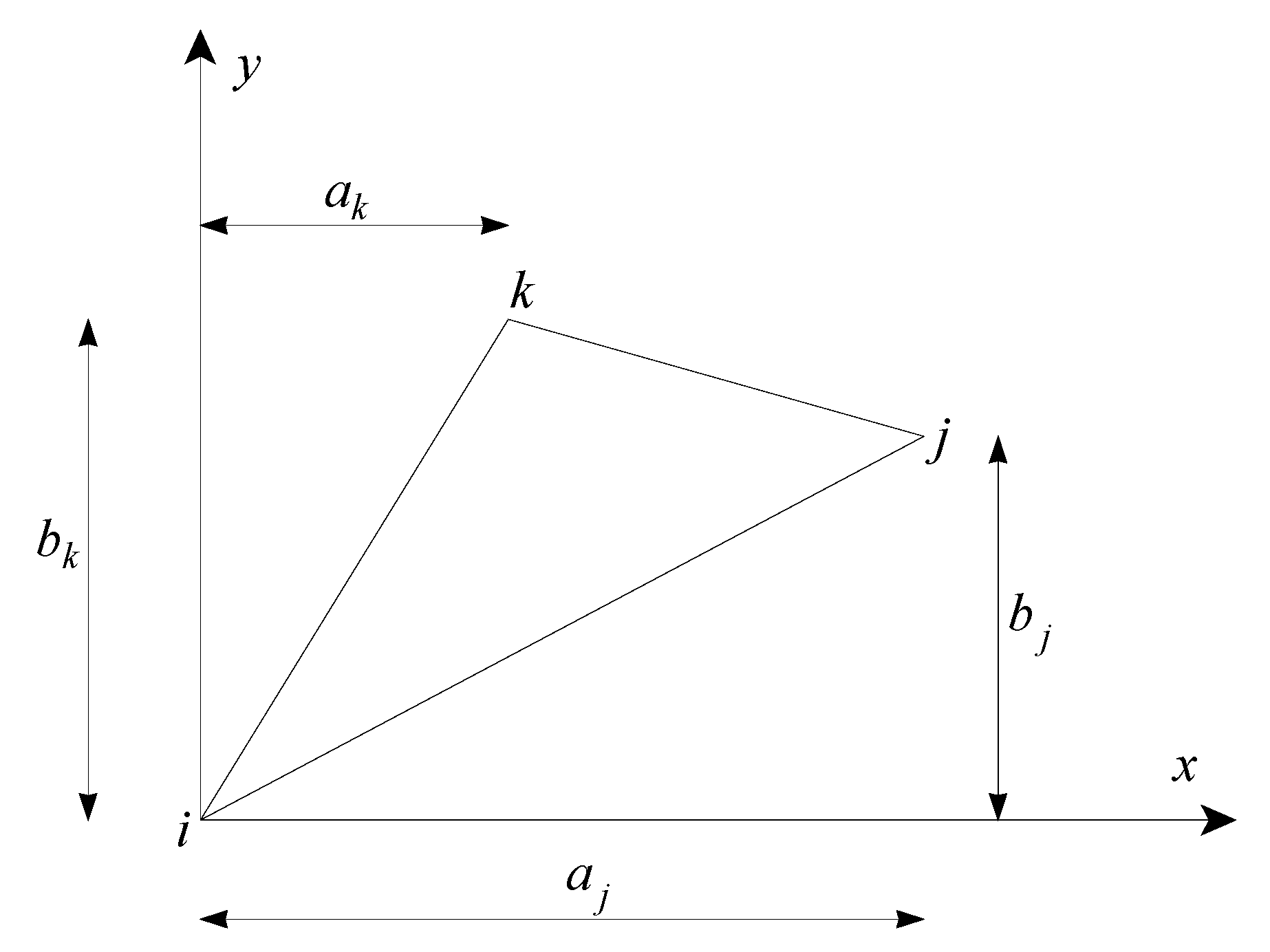
2.1. The Total Potential Energy of Plane Stress Members

It is possible to generate a structural system as a plate problem by considering triangular elements having three nodes i, j, and k, as shown in Figure 1. For the member that has a homogeneous and continuous material, linear displacement fields defined as u(x,y) and v(x,y) are, respectively, given in x and y directions in Equations (1) and (2) for a triangular element in the x-y plane. Translational displacements of a node symbolized as i are shown as u_i and v_i.

$$\mathrm{u}(\mathrm{x},\mathrm{y})={\mathrm{u}}_{\mathrm{i}}+{\mathrm{C}}_1\mathrm{x}+{\mathrm{C}}_2\mathrm{y}$$

(1)

$$\mathrm{v}(\mathrm{x},\mathrm{y})={\mathrm{v}}_{\mathrm{i}}+{\mathrm{C}}_3\mathrm{x}+{\mathrm{C}}_4\mathrm{y}$$

(2)

Knowing the displacement fields including constants named “C₁, C₂, C₃, and C₄,” the strains can be calculated as shown in Equations (3)–(5).

$${\mathsf{\epsilon }}_{\mathrm{x}}=\frac{\partial \mathrm{u}}{\partial \mathrm{x}}={\mathrm{C}}_1$$

(3)

$${\mathsf{\epsilon }}_{\mathrm{y}}=\frac{\partial \mathrm{v}}{\partial \mathrm{y}}={\mathrm{C}}_4$$

(4)

$${\gamma }_{xy}=\frac{\partial u}{\partial y}+\frac{\partial v}{\partial x}=C_2+C_3$$

(5)

The three different strains that are symbolized as ε_x, ε_y, and γ_xy, are the normal strain in the x-direction, normal strain in the y-direction, and shear strain, respectively. The nodal displacements are written as in Equations (6)–(8).

$$\mathrm{u}(0,0)={\mathrm{u}}_{\mathrm{i}},\hspace{0.17em}\hspace{0.17em}\mathrm{v}(0,0)={\mathrm{v}}_{\mathrm{i}}$$

(6)

$$\mathrm{u}({\mathrm{a}}_{\mathrm{j}},{\mathrm{b}}_{\mathrm{j}})={\mathrm{u}}_{\mathrm{j}},\hspace{0.17em}\mathrm{v}({\mathrm{a}}_{\mathrm{j}},{\mathrm{b}}_{\mathrm{j}})={\mathrm{v}}_{\mathrm{j}}$$

(7)

$$\mathrm{u}({\mathrm{a}}_{\mathrm{k}},{\mathrm{b}}_{\mathrm{k}})={\mathrm{u}}_{\mathrm{k}},\hspace{0.17em}\mathrm{v}({\mathrm{a}}_{\mathrm{k}},{\mathrm{b}}_{\mathrm{k}})={\mathrm{v}}_{\mathrm{k}}$$

(8)

After the displacements of each node are obtained, the displacement matrix form can be written as follows using Equations (1) and (2).

$$\left[\begin{array}{c}{u}_j\\ v_j\\ u_k\\ v_k\end{array}\right]=\left[\begin{array}{cccc}{a}_j& b_j& 0& 0\\ 0& 0& a_j& b_j\\ a_k& b_k& 0& 0\\ 0& 0& a_k& b_k\end{array}\right]\left[\begin{array}{c}{C}_1\\ C_2\\ C_3\\ C_4\end{array}\right]+\left[\begin{array}{c}{u}_i\\ v_i\\ u_i\\ v_i\end{array}\right]$$

(9)

In Equations (10)–(13), the constants C₁, C₂, C₃, and C₄ are formulated according to matrix calculations of Equation (9).

$${\mathrm{C}}_1=\frac{{\mathrm{b}}_{\mathrm{k}}({\mathrm{u}}_{\mathrm{j}}-{\mathrm{u}}_{\mathrm{i}})}{{\mathrm{a}}_{\mathrm{j}}{\mathrm{b}}_{\mathrm{k}}-{\mathrm{a}}_{\mathrm{k}}{\mathrm{b}}_{\mathrm{j}}}+\frac{{\mathrm{b}}_{\mathrm{j}}({\mathrm{u}}_{\mathrm{k}}-{\mathrm{u}}_{\mathrm{i}})}{{\mathrm{a}}_{\mathrm{k}}{\mathrm{b}}_{\mathrm{j}}-{\mathrm{a}}_{\mathrm{j}}{\mathrm{b}}_{\mathrm{k}}}$$

(10)

$${\mathrm{C}}_2=\frac{{\mathrm{a}}_{\mathrm{k}}({\mathrm{u}}_{\mathrm{j}}-{\mathrm{u}}_{\mathrm{i}})}{{\mathrm{a}}_{\mathrm{k}}{\mathrm{b}}_{\mathrm{j}}-{\mathrm{a}}_{\mathrm{j}}{\mathrm{b}}_{\mathrm{k}}}+\frac{{\mathrm{a}}_{\mathrm{j}}({\mathrm{u}}_{\mathrm{k}}-{\mathrm{u}}_{\mathrm{i}})}{{\mathrm{a}}_{\mathrm{j}}{\mathrm{b}}_{\mathrm{k}}-{\mathrm{a}}_{\mathrm{k}}{\mathrm{b}}_{\mathrm{j}}}$$

(11)

$${\mathrm{C}}_3=\frac{{\mathrm{b}}_{\mathrm{k}}({\mathrm{v}}_{\mathrm{j}}-{\mathrm{v}}_{\mathrm{i}})}{{\mathrm{a}}_{\mathrm{j}}{\mathrm{b}}_{\mathrm{k}}-{\mathrm{a}}_{\mathrm{k}}{\mathrm{b}}_{\mathrm{j}}}+\frac{{\mathrm{b}}_{\mathrm{j}}({\mathrm{v}}_{\mathrm{k}}-{\mathrm{v}}_{\mathrm{i}})}{{\mathrm{a}}_{\mathrm{k}}{\mathrm{b}}_{\mathrm{j}}-{\mathrm{a}}_{\mathrm{j}}{\mathrm{b}}_{\mathrm{k}}}$$

(12)

$${\mathrm{C}}_4=\frac{{\mathrm{a}}_{\mathrm{k}}({\mathrm{v}}_{\mathrm{j}}-{\mathrm{v}}_{\mathrm{i}})}{{\mathrm{a}}_{\mathrm{k}}{\mathrm{b}}_{\mathrm{j}}-{\mathrm{a}}_{\mathrm{j}}{\mathrm{b}}_{\mathrm{k}}}+\frac{{\mathrm{a}}_{\mathrm{j}}({\mathrm{v}}_{\mathrm{k}}-{\mathrm{v}}_{\mathrm{i}})}{{\mathrm{a}}_{\mathrm{j}}{\mathrm{b}}_{\mathrm{k}}-{\mathrm{a}}_{\mathrm{k}}{\mathrm{b}}_{\mathrm{j}}}$$

(13)

For a body with two dimensions, the strain energy (e) is formulated in Equation (14).

$$e={\displaystyle \underset{\epsilon =0}{\overset{\epsilon }{\int }}\sigma d\epsilon =\frac{1}{2}({\sigma }_x{\epsilon }_x}+{\sigma }_y{\epsilon }_y+{\tau }_{xy}{\gamma }_{xy})$$

(14)

For linear plane strain problems, the stresses are defined as Equations (15)–(17) that include two material constants, namely, elasticity modulus (E) and Poisson’s ratio (ν). σ_x, σ_y, and τ_xy are the normal stress in the x-direction, normal stress in the y-direction, and shear stress, respectively.

$${\sigma }_x=\frac{E}{(1+\nu )(1-2\nu )}((1-\nu ){\epsilon }_x+\nu {\epsilon }_y)$$

(15)

$${\sigma }_y=\frac{E}{(1+\nu )(1-2\nu )}(\nu {\epsilon }_x+(1-\nu ){\epsilon }_y)$$

(16)

$${\tau }_{xy}=\frac{E}{(1+\nu )(1-2\nu )}(\frac{1-2\nu }{2}{\gamma }_{xy})$$

(17)

The strains given as Equations (3)–(5) can be calculated via the constant values formulated as Equations (10)–(13), and then, both strains and stresses are shown in Equations (15)–(17) that used to obtain strain energies using Equation (14) for the linear case. As the main investigation of TPO/MA, three nonlinear stress-strain relationships are formulated as Equations (18)–(20) for Case 1, Equation (21) for Case 2, and Equations (22)–(24) for Case 3. It must be noted that these equations do not necessarily correspond to specific material, and the intention of using these formulations is to demonstrate and test the method that can handle easily.

Case 1. Nonlinear stress-strain relation 1

$${\sigma }_x=\frac{E}{(1+\nu )(1-2\nu )}((1-\nu ){\epsilon }_x^3+\nu {\epsilon }_y)$$

(18)

$${\sigma }_y=\frac{E}{(1+\nu )(1-2\nu )}(\nu {\epsilon }_x+(1-\nu ){\epsilon }_y^3)$$

(19)

$${\tau }_{xy}=\frac{E}{(1+\nu )(1-2\nu )}(\frac{1-2\nu }{2}{\gamma }_{xy})$$

(20)

Case 2. Nonlinear stress-strain relation 2

$$\begin{array}{l}{\sigma }_x=\frac{E}{(1+\nu )(1-2\nu )}((1-\nu ){\epsilon }_x+\nu {\epsilon }_y)\\ {\sigma }_y=\frac{E}{(1+\nu )(1-2\nu )}(\nu {\epsilon }_x+(1-\nu ){\epsilon }_y)\\ {\tau }_{xy}=\frac{E}{(1+\nu )(1-2\nu )}(\frac{1-2\nu }{2}{\gamma }_{xy})\end{array}\}\hspace{0.17em}\hspace{0.17em}\begin{array}{c}\mathrm{for}\hspace{0.17em}\hspace{0.17em}\mathrm{abs}({\epsilon }_x+{\epsilon }_y)<{\epsilon }_0,\hspace{0.17em}\hspace{0.17em}E=E\\ \mathrm{abs}({\epsilon }_x+{\epsilon }_y)>{\epsilon }_0,\hspace{0.17em}\hspace{0.17em}E=0.5E\end{array},$$

(21)

where ε₀ represents a value to control the linearity limit. In numerical examples, it was taken as 0.0001.

Case 3. Nonlinear stress-strain relation 3

$${\sigma }_x=\frac{E}{(1+\nu )(1-2\nu )}{((1-\nu ){\epsilon }_x+\nu {\epsilon }_y)}^3$$

(22)

$${\sigma }_y=\frac{E}{(1+\nu )(1-2\nu )}{(\nu {\epsilon }_x+(1-\nu ){\epsilon }_y)}^3$$

(23)

$${\tau }_{xy}=\frac{E}{(1+\nu )(1-2\nu )}(\frac{1-2\nu }{2}{\gamma }_{xy}^3)$$

(24)

In the formulation of the strain energy of the mth triangular element (U_m) given as Equation (25), strain energy density and volume of the mth triangular element are shown as e_m and V_m, respectively.

$$U_m=e_m{V}_m.$$

(25)

Equation (26) defines the volume of mth triangular element including the constant thickness (t) of the plate under consideration.

$${\mathrm{V}}_{\mathrm{m}}=\frac{({\mathrm{a}}_{\mathrm{j}}{\mathrm{b}}_{\mathrm{k}}-{\mathrm{a}}_{\mathrm{k}}{\mathrm{b}}_{\mathrm{j}})\mathrm{t}}{2}$$

(26)

Then, the total strain energy of a system is calculated by summing the strain energies of all elements generating the system. By calculating the energy for all members defined with the three nodes, as done in examples given in this study, compatibility is automatically provided since the neighbor members are assigned with the corresponding node numbers of the main system, as in FEM applications. As a formulation, the strain energy can be written as in Equation (27) for a system consisting of n elements.

$$\mathrm{U}={\displaystyle \sum _{\mathrm{m}=1}^{\mathrm{n}}{\mathrm{U}}_{\mathrm{m}}}$$

(27)

Finally, the total potential energy (Π_p) that is the difference between work realized with external forces and the total strain energy is calculated via Equation (28) if P_xi and P_yi are the positioned point loads in x and y directions, respectively.

$${\mathsf{\Pi }}_p=U-{\displaystyle \sum _{n=1}^p(P_{xn}{u}_n+P_{yn}{v}_n)}$$

(28)

As an iterative process using an appropriate optimization algorithm, the analysis is handled as a minimization problem of Π_p concerning u_i’s and v_i’s defined as design variables. After finding the nodal displacements, all stresses and strains in the plate are easily determined.

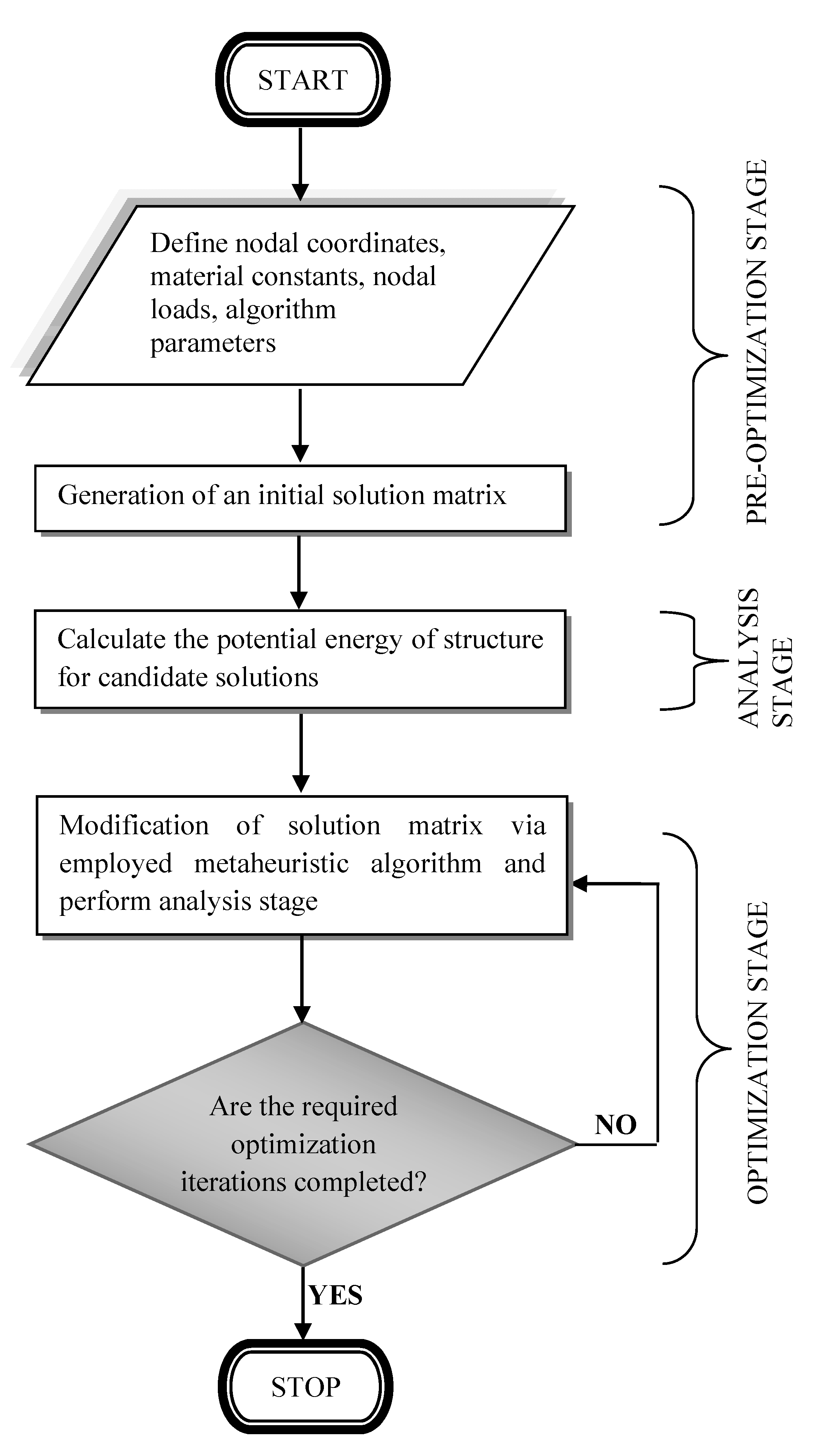
2.2. Optimization Process Via TPO/MA

In the section, the optimization process performed for the minimization of the total potential energy is explained. In the optimization, the objective function is the total potential energy of the system given in Equation (28). It is calculated by summing the energy values of members and subtracting the work done by all external forces.

The flowchart of handling of metaheuristics to provide optimum energy as TPO/MA can be shown in Figure 2.

As with all metaheuristic-based optimization algorithms, the method starts with the definition of nodal coordinates, material constants, nodal loads, and algorithm parameters. The nodes of the system are numbered and the nodal numbers of the members are defined. In that case, it is not needed to define an extra relation for the compatibility of displacements at the nodes. The design variables of the problem are the nodal displacements. For boundary conditions of fixed freedoms, these conditions are taken as design constants and defined as zero. All the other nodal displacements are randomly defined by considering the algorithm rules, and since the displacements are known, it is very practical to calculate directly the energy of all members and then, the whole system. Since the aim of the process is the analysis instead of design, design constraints are not used.

Then, an initial solution vector that includes the candidate values of design variables is generated. These variables are randomly selected in a predefined solution range. In TPO/MA, the design variables are the possible displacements at the nodes of the system that are not correct at the beginning, and then, the exact solution is obtained for the set that has the minimum potential energy value of the system at the end of the iteration process. Once these displacements are set, the distribution of strains in the structure can be defined, followed by the determination of stresses in concordance with the stress-strain relations, whether they are linear or not. Knowing the distribution of stresses and strains, the strain energy at each element can be determined. The summation of all strain energies in the elements gives the total strain energy in the system. Algebraically adding to this value, the work done by external forces due to nodal displacements, the total potential energy of the system becomes calculated. Comparison of these energies calculated for all candidate vectors enables the determination of the best and worst vectors. According to this evaluation, the employed algorithm determines how new candidates will be determined. With this process, one approaches a better set of candidates, and repeatedly following this approach, after several iterations, the final results are obtained.

Nine different metaheuristic algorithms including the genetic-based ones (GA [14], DE [15]), population or nature-based ones (PSO [16], ABC [17,18], FPA [19], TLBO [20], JA [21], GWO [22]), and memory-based HS [23] are evaluated for the linear analysis of the first structural model.

In this study, HS was applied using the modified equations. Here, two different stages exist to find the best harmonies by a musician as given in Equation (29).

$$\{\begin{array}{cc}\begin{array}{c}if \mathrm{HMCR}>\mathrm{rand}( )\\ else\end{array}& \begin{array}{c}{X}_{i, min}+\mathrm{rand} ( )\left(X_{i,max}-X_{i,min}\right)\\ X_{i,n}+\mathrm{rand}\left(\frac{-1}{2},\frac{1}{2}\right)\mathrm{FW} \left(X_{i,max}-X_{i,min}\right)\end{array}\end{array}.$$

(29)

There are two different HS parameters: $\mathrm{HMCR}$ is harmony consideration rate, and $\mathrm{FW}$ is the fret width. $X_{i, min}$ and $X_{i, max}$ are also upper and lower bounds of ith design variable, respectively. On the other hand, $X_{i,n}$ is nth candidate solution and is found as randomly, besides $X_{i, new}$ expresses the new value for this variable.

Also, an adaptive version of HS is employed in the study. To improve the performance of HS, the initial parameters of FW and HMCR are automatically modified during iterations in adaptive HS (AHS) according to Equations (30) and (31). IN and MI represent the current iteration number and maximum iteration number used in optimization, respectively. In addition, a consideration rate was used to allow the best current solution to be more chosen as $X_{i,n}$.

$$\mathrm{FW}={\mathrm{FW}}_{\mathrm{in}}\left(1-\frac{\mathrm{IN}}{\mathrm{MI}}\right)$$

(30)

$$\mathrm{HMCR}={\mathrm{HMCR}}_{\mathrm{in}}\left(1-\frac{\mathrm{IN}}{\mathrm{MI}}\right).$$

(31)

2.3. Structural Models

In the present study, various numerical examples were handled for the optimization of three different structural models. In the analysis process, both linear and three different nonlinear formulations were applied to all structural models. First, a linear analysis was performed on Structure 1 (Section 3.1.1) by employing all of the algorithms, and then, their performance and success were evaluated in terms of approach to the minimum energy value. Then, all structure models were analyzed via the selected algorithm, which has the best performance. Besides, in this process, all optimization analyses are implemented using 100,000 iterations with 30 populations, and 30 cycles for each analysis phase.

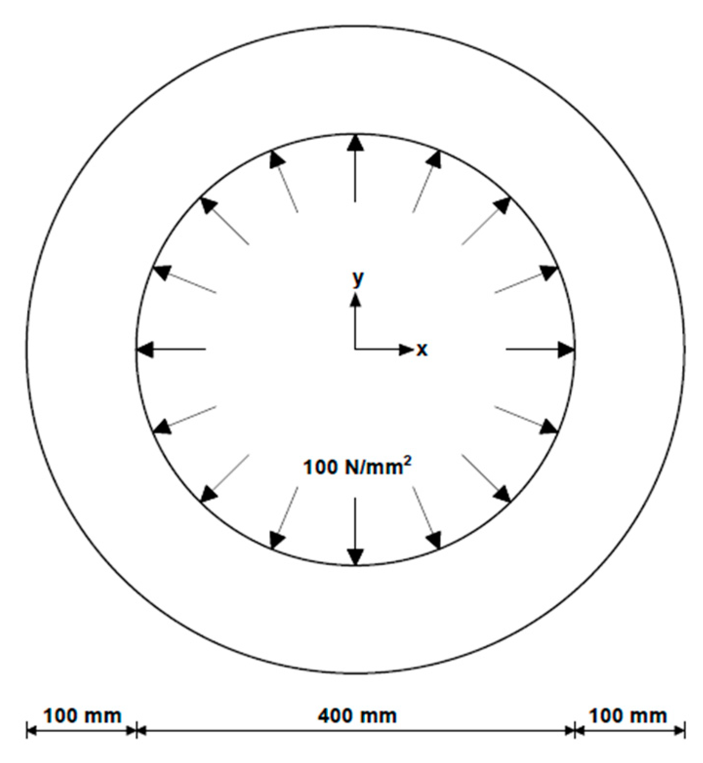
2.3.1. Structure 1: A Pipe with a Thick-Wall Subjected to Internal Pressure

The first model is a pipe structure solved via FEM by Topçu [24]. It has walls with 100 mm thickness under the effect of internal pressure. The internal pressure is 100 N/mm² as seen in Figure 3. Elasticity modulus and Poisson’s ratio of pipe used are 100 kN/mm² and 0.25, respectively, as reported in Topçu [24]. It can be shown that the model can be handled using a quarter of it with 4 members and 6 nodes due to the symmetry of the pipe as shown in Figure 4.

The same problem was analyzed for a finer meshing option. Similarly, it is analyzed as a quarter system using a different meshing model. This mesh difference is related to the use of members and node numbers as 12 and 14, respectively, in Figure 5.

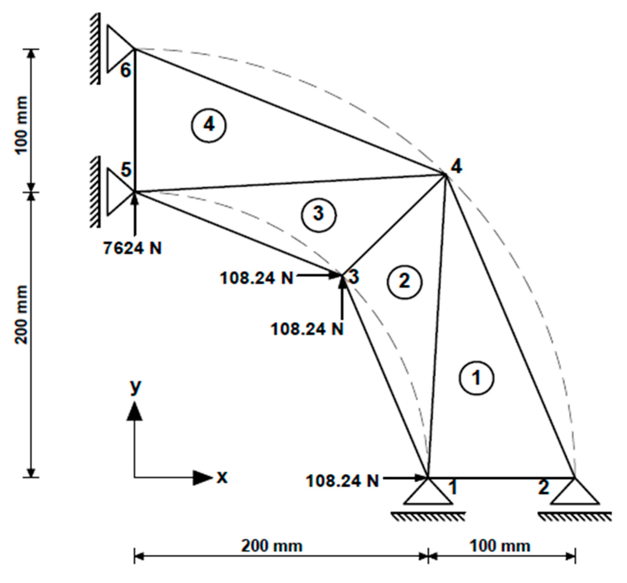
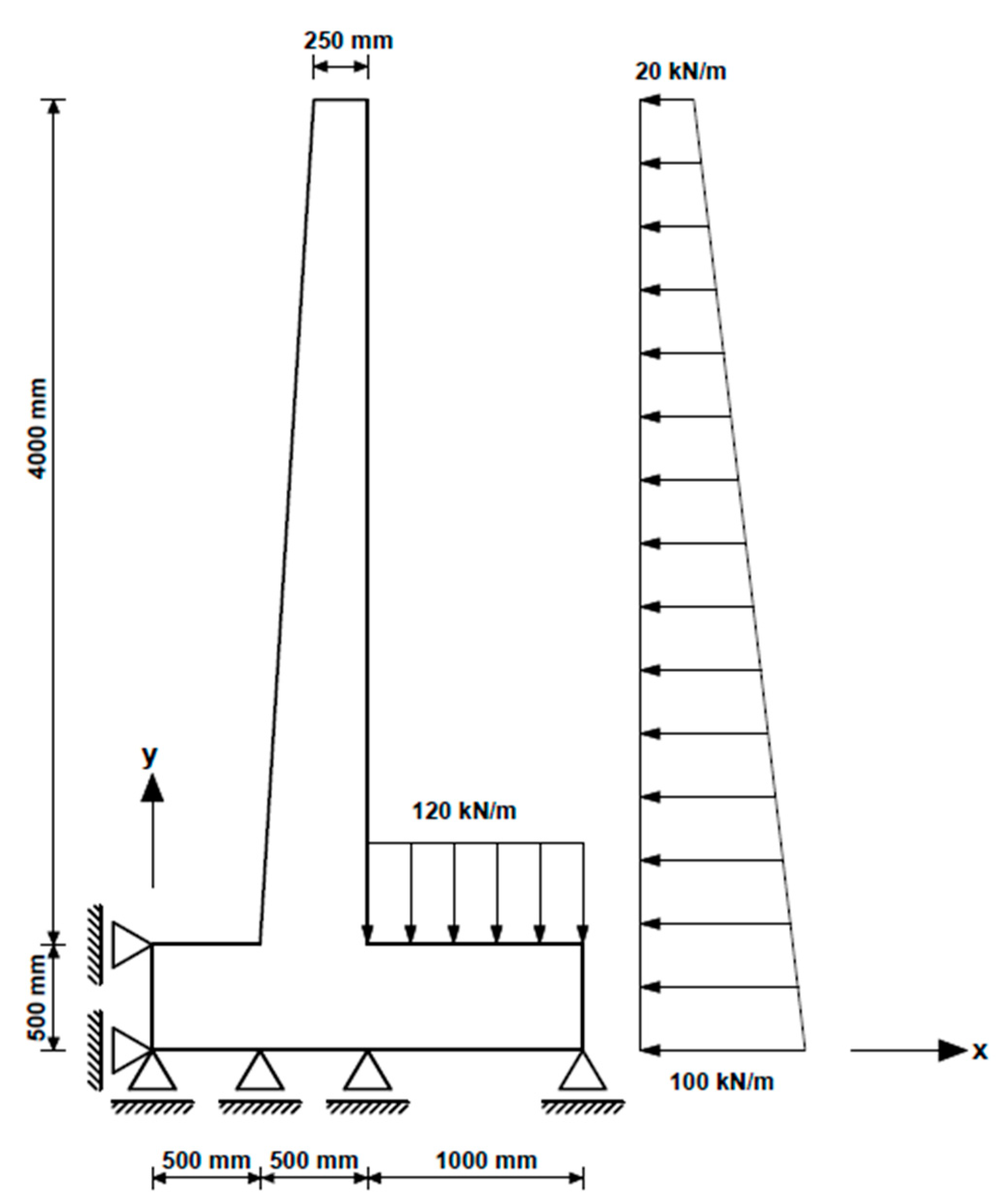
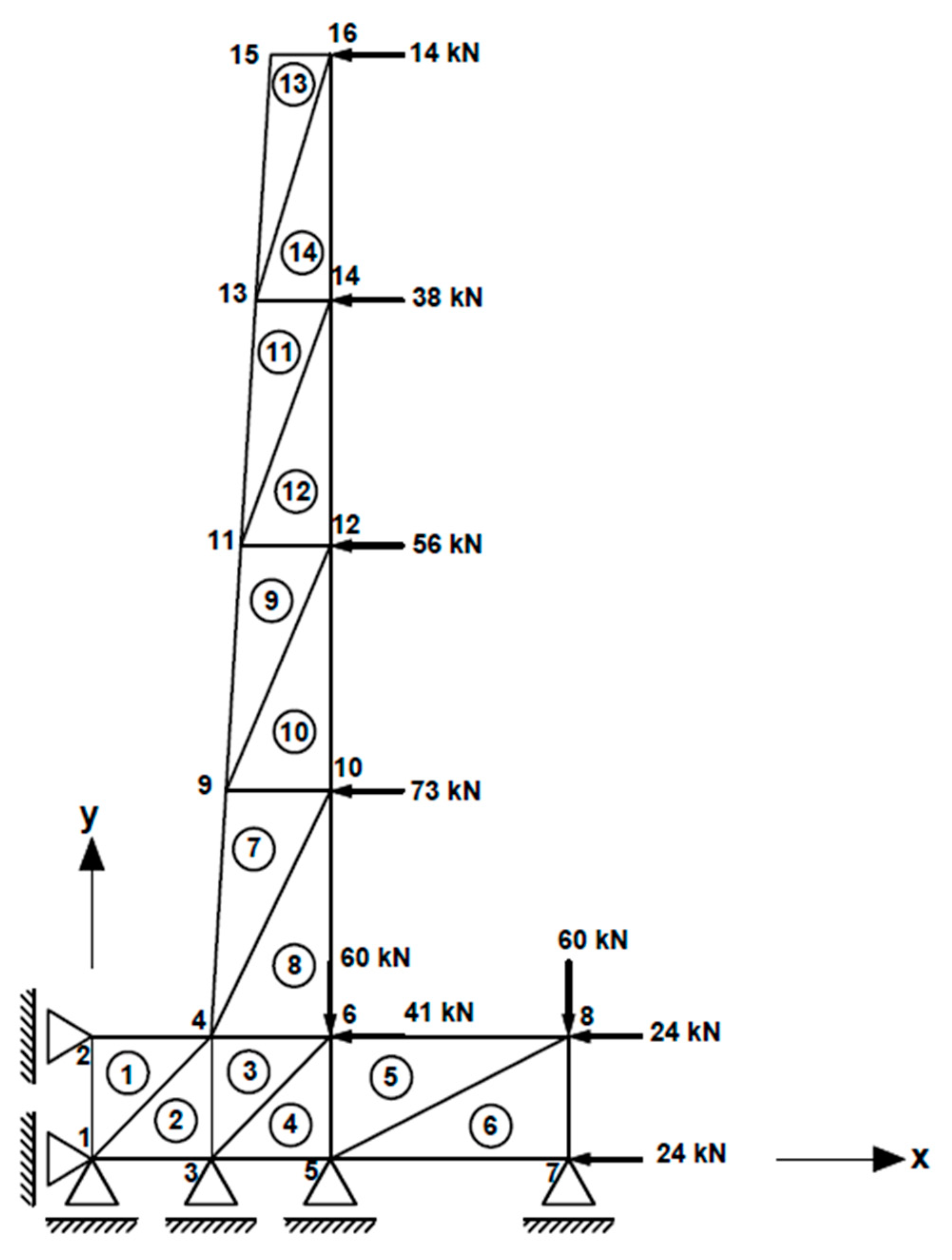
2.3.2. Structure 2: A Cantilever Retaining Wall (with 14 Members-16 Nodes)

Finally, the third structural model is a reinforced concrete (RC) cantilever retaining wall (Structure 2). The model is shown in Figure 6 with the loading conditions. Additionally, the model is generated with a meshing of the system by considering 14 members-16 nodes in Figure 7. Properties of an RC cantilever retaining wall material are selected as 32 × 10⁶ kN/m² and 0.2 for the elasticity modulus (E) and Poisson’s ratio, respectively.

3. Results

3.1. Structure 1

3.1.1. Linear Analysis to Evaluate Nine Employed Metaheuristics

This case aims to find the best suitable algorithm for the problem to apply this algorithm to advance and nonlinear cases. The optimization results provided by nine algorithms for the present structure are represented in

Table 1. Optimization results for the structural system with 4 members-6 nodes (linear).

TPOMA
Method	Node 1		Node 2		Node 3		Node 4		Node 5		Node 6		Пp (Nmm)
	Δx (mm)	Δy (mm)	Δx (mm)	Δy (mm)	Δx (mm)	Δy (mm)	Δx (mm)	Δy (mm)	Δx (mm)	Δy (mm)	Δx (mm)	Δy (mm)
FEM	0.472	0.000	0.424	0.000	0.370	0.370	0.297	0.297	0.000	0.472	0.000	0.424	−7611.581
GA	2.208	0.000	2.239	0.000	1.521	0.054	1.168	0.131	0.000	−0.698	0.000	−0.980	34,413.583
DE	0.472	0.000	0.424	0.000	0.370	0.370	0.297	0.297	0.000	0.472	0.000	0.424	−7611.581
PSO	0.393	0.000	0.335	0.000	0.329	0.430	0.272	0.336	0.000	0.577	0.000	0.529	−7511.990
HS	0.471	0.000	0.424	0.000	0.369	0.362	0.294	0.290	0.000	0.474	0.000	0.424	−7607.300
AHS	0.472	0.000	0.424	0.000	0.370	0.370	0.297	0.297	0.000	0.472	0.000	0.424	−7611.581
ABC	−0.389	0.000	−0.486	0.000	−0.185	0.325	−0.039	0.320	0.000	0.492	0.000	0.461	470.741
TLBO	0.472	0.000	0.424	0.000	0.370	0.370	0.297	0.297	0.000	0.472	0.000	0.424	−7611.581
FPA	0.472	0.000	0.424	0.000	0.370	0.370	0.297	0.297	0.000	0.472	0.000	0.424	−7611.581
GWO	−0.656	0.000	0.037	0.000	−0.400	−2.337	0.816	−2.336	0.000	0.048	0.000	−0.553	359,953.164
JA	0.472	0.000	0.424	0.000	0.370	0.370	0.297	0.297	0.000	0.472	0.000	0.424	−7611.581

. From the table, the most effective and successful algorithms are AHS, DE, TLBO, FPA, and JA in terms of approaching minimum energy. FEM can be easily and directly applied to linear systems to find the exact solutions, and the solution of nodal displacements is the same for FEM results reported in Topçu [24] and the mentioned successful algorithms. The essential advantage of TPOMA is the solving ability of nonlinear systems without implementations of an additional method, while FEM needs to be combined with other iterative methods to solve a specific nonlinear case.

Besides, the best iteration steps from all iterations in each cycle were evaluated with the direction of providing the best objective function in

Table 2. Evaluation of best iteration steps among maximum iteration numbers to reach the minimum total energy.

Best Methods	Пp (Nmm)	Mean of Пp (Nmm)	Standard Deviation of Пp (Nmm)	Best Iteration
DE	−7611.581	−7611.581	0.000000000002	93,515
TLBO	−7611.581	−7611.581	0.000000000002	4882
FPA	−7611.581	−7611.581	0.000000000002	2824
JA	−7611.581	−7611.581	0.000000000002	10,698
AHS	−7611.581	−7611.581	0.000000000002	2023

. The total potential energies, i.e., the best and average values, and the standard deviations are the same for the best 5 methods. The following analyses are conducted via AHS since this method was arriving at the best total potential energy with the least number of iterations, as compared to the other algorithms, as can be seen in Table 2.

3.1.2. Nonlinear Analysis by Employing AHS

For nonlinear cases, the nodal displacement and minimum total potential energy are presented in

Table 3. Optimum solutions for the system with 4 members-6 nodes (adaptive harmony search (AHS)).

	TPOMA (linear)		TPOMA (Nonlinear 1)		TPOMA (Nonlinear 2)		TPOMA (Nonlinear 3)
Node	Δx (mm)	Δy (mm)	Δx (mm)	Δy (mm)	Δx (mm)	Δy (mm)	Δx (mm)	Δy (mm)
1	0.475	0	24.576	0	0.9436	0.0000	24.2151	0.0000
2	0.424	0	−13.677	0	0.8473	0.0000	15.3721	0.0000
3	0.370	0.370	79.170	79.170	0.7392	0.7392	24.4123	24.4124
4	0.297	0.297	74.359	74.359	0.5936	0.5936	24.1185	24.1185
5	0	0.472	0	24.576	0.0000	0.9436	0.0000	24.2157
6	0	0.424	0	−13.677	0.0000	0.8473	0.0000	15.3726
Пp (Nmm)	−7611.581		−7.3478558728 × 107		−15,223.1614		−674,376.1117

. The example has only 8 non-zero displacements. That is why the method is presented for a higher number of freedoms than structure 1 in other numerical examples. The nonlinear constitutive equations used in the paper show that the nonlinear stress-strain relationship in case 2 is very close to one in the linear case, while the other 2 relationships corresponding to case 1 and case 3 are very different from the one in the linear case. Cases 1 and 3 involve cubic powers of the strain on the right-hand side of the equations, while the only difference between nonlinear case 2 and linear relationships is the shifting of the value of the elasticity modulus according to the values of strains. In numerical examples, the value of elasticity modulus for the nonlinear part of case 2 is half of the linear case. It seems that the strains generally tend to the nonlinear part with the half elasticity modulus value that is resulted in the doubling of displacements compared to the linear case. Similarly, the total potential energy value in case 2 is double than in the linear case, while the other nonlinear cases have very small total potential energy values. All total potential energies are negative, and the absolute values of the total potential energy show an increase with the direct increase in the nodal displacements.

To verify the nonlinear cases, Poisson’s ratio values are checked between 0.27 and 0.3 for all cases and the results are presented in

Table 4. Optimum solutions for the system with 4 members-6 nodes for different Poisson’s ratio values (nonlinear via AHS).

ν		TPOMA (Linear)		TPOMA (Nonlinear 1)		TPOMA (Nonlinear 2)		TPOMA (Nonlinear 3)
	Node	Δx (mm)	Δy (mm)	Δx (mm)	Δy (mm)	Δx (mm)	Δy (mm)	Δx (mm)	Δy (mm)
0.27	1	0.4694	0.0000	25.6721	0.0000	0.9389	0.0000	20.1678	0.0000
	2	0.4171	0.0000	−14.9597	0.0000	0.8341	0.0000	10.1456	0.0000
	3	0.3696	0.3696	85.3729	85.3729	0.7392	0.7392	28.1996	28.1996
	4	0.2920	0.2920	79.8247	79.8247	0.5841	0.5841	26.3712	26.3712
	5	0.0000	0.4694	0.0000	25.6721	0.0000	0.9389	0.0000	20.1678
	6	0.0000	0.4171	0.0000	−14.9597	0.0000	0.8341	0.0000	10.1456
	Пp (Nmm)	−7593.8609		−101,203,819.3376		−15,187.7219		−689,396.1522
0.28	1	0.4681	0.0000	26.2344	0.0000	0.9362	0.0000	19.5071	0.0000
	2	0.4136	0.0000	−15.5831	0.0000	0.8273	0.0000	9.0151	0.0000
	3	0.3696	0.3696	88.4359	88.4359	0.7391	0.7391	29.2697	29.2697
	4	0.2895	0.2895	82.5355	82.5355	0.5791	0.5791	27.1497	27.1497
	5	0.0000	0.4681	0.0000	26.2344	0.0000	0.9362	0.0000	19.5071
	6	0.0000	0.4136	0.0000	−15.5831	0.0000	0.8273	0.0000	9.0151
	Пp (Nmm)	−7583.2397		−118,167,986.0712		−151,66.4795		−699,183.7821
0.29	1	0.4667	0.0000	26.8047	0.0000	0.9334	0.0000	19.0866	0.0000
	2	0.4101	0.0000	−16.1982	0.0000	0.8202	0.0000	8.1306	0.0000
	3	0.3695	0.3695	91.4805	91.4805	0.7390	0.7390	30.2294	30.2294
	4	0.2869	0.2869	85.2366	85.2366	0.5739	0.5739	27.9006	27.9006
	5	0.0000	0.4667	0.0000	26.8047	0.0000	0.9334	0.0000	19.0866
	6	0.0000	0.4101	0.0000	−16.1982	0.0000	0.8202	0.0000	8.1306
	Пp (Nmm)	−7571.4371		−137,625,581.0665		−15,142.8743		−709,938.7099
0.30	1	0.4652	0.0000	27.3819	0.0000	0.9304	0.0000	18.7847	0.0000
	2	0.4064	0.0000	−16.8072	0.0000	0.8128	0.0000	7.3561	0.0000
	3	0.3694	0.3694	94.5115	94.5115	0.7387	0.7387	31.1627	31.1627
	4	0.2843	0.2843	87.9316	87.9316	0.5686	0.5686	28.6625	28.6625
	5	0.0000	0.4652	0.0000	27.3819	0.0000	0.9304	0.0000	18.7847
	6	0.0000	0.4064	0.0000	−16.8072	0.0000	0.8128	0.0000	7.3561
	Пp (Nmm)	−7558.4473		−159,977,948.1027		−15,116.8946		−721,624.5843

. For the linear case and nonlinear case 2, the effect of the Poisson’s ratio is limited. In the linear case, the percentage of change of energies is 0.47% by considering minimum and maximum energies. The same value for nonlinear case 2 is 0.47%. For the other cases, the increases of Poisson’s ratio significantly affect both displacement and total potential energy values. It is observed that the absolutes of the total potential energy values show an increase with the increase in Poisson’s ratio. The increase in absolute displacement values in nonlinear case 1 is directly proportional to that of the Poisson’s ratio and the difference ratio between maximum and minimum energies is 36.74%. In nonlinear case 3 where the cubic powers are also included for the Poisson’s ratio values, specific displacements increase, while other ones show a decreasing manner by the increase in the Poisson’s ratio values. The maximum percentage difference of total potential energy values is 4.47% for this case.

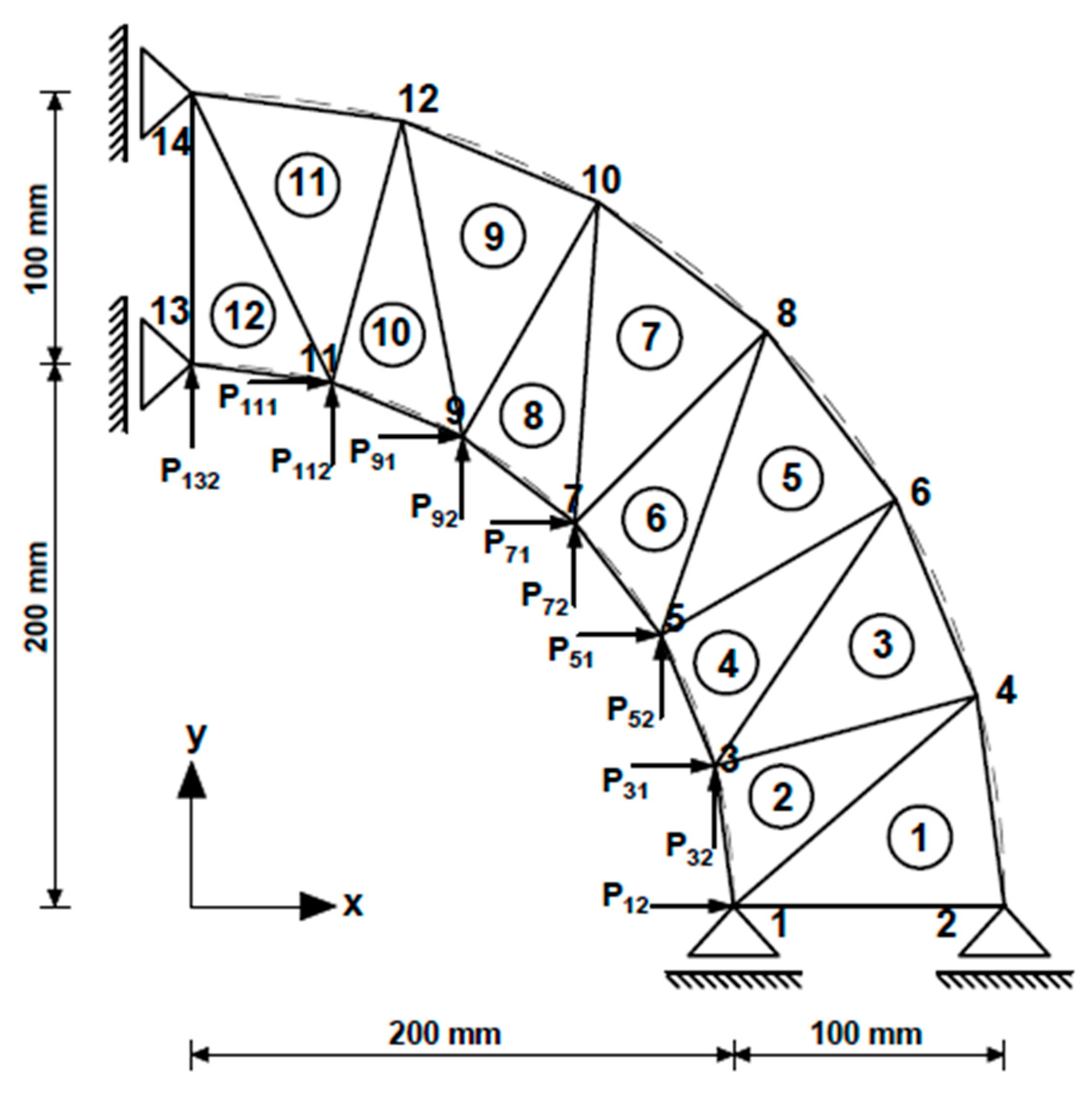
3.1.3. Advanced Case of Structure 1 with 12 Members-14 Nodes

The applied loads on nodes for this meshing option can be seen in

Table 5. Applied concentrated loads for Structure 2.

	Concentrated Loads (N)
Node	x Direction	y Direction
1	P11 = 2610.5	P12 = 171.1
3	P31 = 5043.1	P32 = 1351.3
5	P51 = 4521.6	P52 = 2610.5
7	P71 = 3691.8	P72 = 3691.8
9	P91 = 2610.5	P92 = 4521.6
11	P111 = 1351.3	P112 = 5043.1
13	P113 = 171.1	P113 = 2610.5

.

The results of the analyses are shown in

Table 6. Optimum results for the system with 12 members-14 nodes (AHS).

	FEM (Linear)		TPOMA (Linear)		TPOMA (Nonlinear 1)		TPOMA (Nonlinear 2)		TPOMA (Nonlinear 3)
Node	Δx (mm)	Δx (mm)	Δx (mm)	Δy (mm)	Δx (mm)	Δy (mm)	Δx (mm)	Δy (mm)	Δx (mm)	Δy (mm)
1	0.479	0.000	0.479	0.000	29.882	0.000	0.959	0.000	27.652	0.000
2	0.422	0.000	0.422	0.000	−0.219	0.000	0.845	0.000	20.305	0.000
3	0.480	0.131	0.480	0.131	40.580	25.3407	0.961	0.261	28.044	9.018
4	0.404	0.104	0.404	0.104	8.190	18.872	0.807	0.208	18.110	6.868
5	0.442	0.254	0.442	0.254	59.811	53.252	0.883	0.508	28.741	18.130
6	0.368	0.210	0.368	0.210	40.500	48.925	0.736	0.420	21.545	16.379
7	0.373	0.373	0.373	0.373	86.303	86.303	0.746	0.746	24.585	24.585
8	0.294	0.294	0.294	0.294	84.501	84.501	0.588	0.588	25.376	25.376
9	0.254	0.442	0.254	0.442	53.252	59.811	0.508	0.883	18.130	28.741
10	0.210	0.368	0.210	0.368	48.925	40.500	0.420	0.736	16.379	21.545
11	0.131	0.480	0.131	0.480	25.341	40.580	0.261	0.961	9.018	28.044
12	0.104	0.404	0.104	0.404	18.872	8.190	0.208	0.807	6.868	18.110
13	0.000	0.479	0.000	0.479	0	29.882	0.000	0.959	0.000	27.652
14	0.000	0.422	0.000	0.422	0	−0.219	0.000	0.845	0.000	20.305
Пp (Nmm)			−7887.851		−1.09356257515 × 108		−15,775.702		−740,764.295

. From the table, optimization results of the linear analysis are closely compared with the first meshing option in Figure 4. The displacement results show a great match with the FEM results for the linear case. However, nonlinear analysis results are very different from this structure, especially for nonlinear cases as 1 and 3. Besides that, in this model, energies can be provided less than the first model. Similar behavior with the other meshing option is observed as expected for the comparison of linear and nonlinear cases.

3.2. Structure 2

The ensured optimum analysis results are shown in

Table 7. Solutions for the system with 14 members (AHS).

	FEM (Linear)	TPOMA (Linear)			TPOMA (Nonlinear 1)		TPOMA (Nonlinear 2)		TPOMA (Nonlinear 3)
Node	Δx (m)	Δy (m)	Δx (m)	Δy (m)	Δx (m)	Δy (m)	Δx (m)	Δy (m)	Δx (m)	Δy (m)
1	0.000000	0.000000	0.000000	0.000000	0.000000	0.000000	0.000000	0.000000	0.000000	0.000000
2	0.000000	−0.000002	0.000000	−0.000002	0.000000	−0.176510	0.000000	−0.000002	0.000000	−0.002403
3	−0.000002	0.000000	−0.000002	0.000000	0.176644	0.000000	−0.000002	0.000000	−0.002019	0.000000
4	−0.000010	−0.000014	−0.000010	−0.000014	−0.177006	−0.177006	−0.000010	−0.000014	−0.013126	−0.012299
5	−0.000013	0.000000	−0.000013	0.000000	0.353080	0.000000	−0.000013	0.000000	−0.017347	0.000000
6	−0.000014	0.000011	−0.000014	0.000011	0.353137	−0.176261	−0.000014	0.000011	−0.022839	0.014085
7	−0.000018	0.000000	−0.000018	0.000000	0.706119	0.000000	−0.000018	0.000000	−0.035964	0.000000
8	−0.000020	0.000000	−0.000020	0.000000	0.706354	−0.177103	−0.000020	0.000000	−0.042223	0.005558
9	−0.000140	−0.000032	−0.000141	−0.000032	0.193755	−0.531293	−0.000140	−0.000032	−0.118902	−0.024612
10	−0.000139	0.000036	−0.000140	0.000036	0.349492	−0.528870	−0.000138	0.000036	−0.112289	0.035232
11	−0.000340	−0.000031	−0.000342	−0.000032	0.211354	−0.884866	−0.000339	−0.000031	−0.283322	−0.027028
12	−0.000339	0.000047	−0.000341	0.000047	0.342311	−0.881895	−0.000338	0.000047	−0.278773	0.042540
13	−0.000573	−0.000022	−0.000576	−0.000023	0.224691	−1.237878	−0.000571	−0.000022	−0.492982	−0.024042
14	−0.000573	0.000050	−0.000576	0.000050	0.334289	−1.235242	−0.000571	0.000050	−0.490333	0.045575
15	−0.000814	−0.000009	−0.000818	−0.000009	0.237355	−1.590342	−0.000811	−0.000009	−0.730701	−0.015649
16	−0.000814	0.000051	−0.000818	0.000051	0.325597	−1.588350	−0.000811	0.000051	−0.729844	0.042830
Пp (kNm)			−0.031567	−1,385,982.025122			−0.031567		−40.719902

. As expected, linear and nonlinear results are different from each other. The linear results of FEM show a good match with those of TPO/MA. Both displacement and total potential energy of the second nonlinear case are the same as those of the linear case since all deformations are within the limitation of the linearity. Different from the other example, the strain values of nonlinear case 2 are the same as those of the linear case because the linearity limit used in nonlinear case 2 was not exceeded. The same structure was analyzed for different Poisson’s ratio values, and the minimum total potential energy values are shown in

Table 8. The total energy values for the system with 14 members by changing Poisson’s ratio (AHS).

ν	TPOMA (Linear)	TPOMA (Nonlinear 1)	TPOMA (Nonlinear 2)	TPOMA (Nonlinear 3)
0.15	−0.031403525	−654458.4484	−0.031403525	−39.59712014
0.16	−0.031457332	−771097.8575	−0.031457332	−39.81729795
0.17	−0.031501216	−900090.841	−0.031501216	−40.03945641
0.18	−0.031534625	−1044225.23	−0.031534625	−40.26378793
0.19	−0.031556952	−1205801.743	−0.031556952	−40.49051621
0.2	−0.031567536	−1385982.025	−0.031567536	−40.71990187
0.21	−0.031565648	−1586562.796	−0.031565648	−40.95224928
0.22	−0.031550489	−1812681.81	−0.031550489	−41.18791476

. From the results, the changes of Poisson’s ratio have a small effect on the values for the cases with a small absolute value of the total potential energy. Although the results of nonlinear case 1 show a linear and expected reduction by the increase in the Poisson’s ratio, the effects are significant due to big energy values in absolute value. The different percentages of maximum and minimum energy values are 0.52%, 63.90%, 0.52%, and 3.86% for the linear case, nonlinear case1, nonlinear case2, and nonlinear case3, respectively.

4. Discussions

In the present study, the best method in finding the minimum potential energy level is found to be AHS. Methods taken into account are compared with each other according to their performance in solving the verification case, which is the 4 member model of pipe example. Five of 10 algorithms are found to be effective in finding the optimum value. Their robustness is checked by solving the same problem 30 times and evaluating the results obtained in all these runs. It has been seen in this evaluation that all these algorithms were robust giving nearly zero standard deviation values. The essential advantage of AHS was the computing time. Indeed, AHS could reach the optimum results with 2023 iterations, while for DE, TLBO, FPA, and JA, the number of iterations was 93513, 4882, 2824, and 10698, respectively.

After finding the best method, the nonlinear cases were handled by only changing the employed equations for the stress-strain relationship. It is seen that, as expected, there were no difficulties in solving these nonlinear problems once relevant stress-strain equations are used.

5. Conclusions

In the present study, it is shown that TPO/MA is an efficient method in solving plane strain problems too whether the constitutive equation is linear or not.

Until now, TPO/MA was applied to truss systems [5,6,7,8], tensegrity structures [9], cable structures [10,11], and plane stress problems [12,13] for a wide range of examples. By including plane-strain problems in the application record, it is shown in this paper that the application area of this technique is not limited to previous ones. It is hoped that in the future, the method TPO/MA will be shown to apply to many other types of structural analysis problems.

Currently, there are quite a big number of metaheuristic algorithms. Although all of them can be implemented in TPO/MA, it is seen that there may be differences in inaccuracies and time consumed, probably depending on problems. In this paper, 10 metaheuristic algorithms were compared with each other on an exemplary problem that was a 4 member pipe with a linear stress-strain relationship. It is seen that among the algorithms tried, five were more efficient than the others, and AHS among them was the most successful if the CPU time is taken into account.

Three different nonlinear behaviors are reflected with stress-strain relationships that are different from the linear material. The nonlinear stress-strain relations in case 2 are very close to those of the linear case since it differs from the linear problem by only with the shifting of the value of the elasticity modulus according to the values of strains. For example, displacements of nonlinear case 2 in structure 1 were double those in the linear case due to the tendency of the nonlinear part with the half value of the elasticity modulus of the linear situation. Differently, displacements in nonlinear case 2 of structure 2 tend to have the same value of the elasticity modulus of the linear case. Both displacements and total potential energy of nonlinear case 1 and case 3 are very different from those of linear case since these cases involve cubic powers.

The method TPO/MA can automatically deal with nonlinear stress-strain relationship formulations by only changing the coded equation without the need for additional user interventions like in FEM. In addition, TPO/MA can handle the total potential energy process quickly. For example, the process for the linear case of structure 1 via AHS can reach the optimum solution after 0.4 s of computing time.

As indicated above, the nonlinear analyses were done by employing AHS after seeing its success in applications on the linear case. Indeed, it was among the five algorithms that reached the minimum energy level in all cycles, and the one necessitating minimum CPU time. For nonlinear cases, the processing time is between 1 and 2 s according to the number of design variables.

This study has shown that TPO/MA is a real and powerful alternative to other methods in solving statical analysis problems especially when there are nonlinearities in the problem. In future researches, complex systems; especially space structures can be constructed as plane stress or plane strain members can be solved via the proposed method to increase the generality of TPOMA. As more complexity than the existing ones, the plate member that include rotational freedoms and those which are under-constrained can be considered. Via this capacity, it will be possible to make the full detailed analysis of a structure using a single method.

References

1. Saffari, H.; Fadaee, M.J.; Tabatabaei, R. Nonlinear Analysis of Space Trusses Using Modified Normal Flow Algorithm. J. Struct. Eng. 2008, 134, 998–1005. [Google Scholar] [CrossRef]
2. Krenk, S. Non-Linear Modeling and Analysis of SOLIDS and Structures; Cambridge University Press: Cambridge, UK, 2009. [Google Scholar]
3. Greco, M.; Menin, R.; Ferreira, I.; Barros, F. Comparison between two geometrical nonlinear methods for truss analyses. Struct. Eng. Mech. 2012, 41, 735–750. [Google Scholar] [CrossRef]
4. Levy, R.; Spillers, W.R. Analysis of Geometrically Nonlinear Structures; Springer Science & Business Media: Berlin, Germany, 2013. [Google Scholar]
5. Toklu, Y.C. Nonlinear analysis of trusses through energy minimization. Comput. Struct. 2004, 82, 1581–1589. [Google Scholar] [CrossRef]
6. Toklu, Y.C.; Bekdaş, G.; Nigdeli, S.M. Analysis of under-constrained and unstable structures by the method TPO/MA. In Proceedings of the 15th International Conference of Numerical Analysis and Applied Mathematics, Thessaloniki, Greece, 25–30 September 2017. [Google Scholar]
7. Kayabekir, A.E.; Bekdaş, G.; Nigdeli, S.M.; Toklu, Y.C. The Population Factor on Metaheuristic Based Analyses of Truss Structures. In Proceedings of the International Conference on Bioinspired Optimization Methods and their Applications (BIOMA 2018), Paris, France, 16–18 May 2018. [Google Scholar]
8. Bekdaş, G.; Kayabekir, A.E.; Nigdeli, S.M.; Toklu, Y.C. Advanced energy-based analyses of trusses employing hybrid metaheuristics. Struct. Des. Tall Spéc. Build. 2019, 28, e1609. [Google Scholar] [CrossRef]
9. Toklu, Y.C.; Uzun, F. Analysis of tensegric structures by total potential optimization using metaheuristic algorithms. J. Aerosp. Eng. 2016, 29, 04016023. [Google Scholar] [CrossRef]
10. Bekdaş, G.; Kayabekir, A.E.; Nigdeli, S.M.; Toklu, Y.C. Analyses of cable nets by using energy minimization using several metaheuristic methods. In Proceedings of the International Conference on Bioinspired Optimization Methods and their Applications (BIOMA 2018), Paris, France, 16–18 May 2018. [Google Scholar]
11. Nigdeli, S.M.; Bekdaş, G.; Toklu, Y.C. Total Potential Energy Minimization Using Metaheuristic algorithms for Spatial Cable Systems with increasing Second Order Effects. In Proceedings of the 12th International Congress on Mechanics (HSTAM2019), Thessaloniki, Greece, 22–25 September 2019. [Google Scholar]
12. Kayabekir, A.E.; Toklu, Y.C.; Bekdaş, G.; Nigdeli, S.M.; Yücel, M.; Geem, Z.W. A Novel Hybrid Harmony Search Approach for the Analysis of Plane Stress Systems via Total Potential Optimization. Appl. Sci. 2020, 10, 2301. [Google Scholar] [CrossRef] [Green Version]
13. Toklu, Y.C.; Kayabekir, A.E.; Bekdaş, G.; Nigdeli, S.M.; Yücel, M. Analysis of Plane-Stress Systems via Total Potential Optimization Method Considering Nonlinear Behavior. J. Struct. Eng. 2020, 146, 04020249. [Google Scholar] [CrossRef]
14. Holland, J.H. Adaptation in Natural and Artificial Systems; University of Michigan Press: Ann Arbor, MI, USA, 1975. [Google Scholar]
15. Storn, R.; Price, K. Differential Evolution–A Simple and Efficient Heuristic for global Optimization over Continuous Spaces. J. Glob. Optim. 1997, 11, 341–359. [Google Scholar] [CrossRef]
16. Eberhart, R.; Kennedy, J. Particle swarm optimization. In Proceedings of the IEEE International Conference on Neural Networks, Perth, WA, Australia, 27 November–1 December 1995; Volume 4, pp. 1942–1948. [Google Scholar]
17. Karaboga, D. An Idea Based on Honey Bee Swarm for Numerical Optimization; Technical Report-tr06; Erciyes University, Engineering Faculty, Computer Engineering Department: Kayseri, Turkey, 2005; Volume 200, pp. 1–10. [Google Scholar]
18. Karaboga, D.; Basturk, B. Artificial Bee Colony (ABC) Optimization Algorithm for Solving Constrained Optimization Problems. In Proceedings of the International Fuzzy Systems Association World Congress, Cancun, Mexico, 27–30 June 2007; Springer: Berlin/Heidelberg, Germany; pp. 789–798. [Google Scholar]
19. Rao, R.V.; Savsani, V.J.; Vakharia, D.P. Teaching–learning-based optimization: A novel method for constrained mechanical design optimization problems. Comput. Aided Des. 2011, 43, 303–315. [Google Scholar] [CrossRef]
20. Yang, X.S. Flower pollination algorithm for global optimization. In Proceedings of the International Conference on Unconventional Computing and Natural Computation, Orléans, France, 3–7 September 2012; Springer: Berlin/Heidelberg, Germany, 2012; pp. 240–249. [Google Scholar]
21. Mirjalili, S.; Mirjalili, S.M.; Lewis, A. Grey wolf optimizer. Adv. Eng. Softw. 2014, 69, 46–61. [Google Scholar] [CrossRef] [Green Version]
22. Rao, R.V. Jaya: A simple and new optimization algorithm for solving constrained and unconstrained optimization problems. Int. J. Ind. Eng. Comput. 2016, 7, 19–34. [Google Scholar]
23. Geem, Z.W.; Kim, J.H.; Loganathan, G.V. A new heuristic optimization algorithm: Harmony search. Simulation 2001, 76, 60–68. [Google Scholar] [CrossRef]
24. Topçu, A. Sonlu Elemanlar Metodu, Eskişehir Osmangazi Üniversitesi. 2015. Available online: http://mmf2.ogu.edu.tr/atopcu/ (accessed on 1 April 2019).
Figure 1. Triangular elements used in the generation of plate systems.
Applsci 11 03220 g001
Figure 2. The flowchart of the Total Potential Optimization using Metaheuristic Algorithms (TPO/MA) including three stages used in the process.
Applsci 11 03220 g002
Figure 3. Structure 1: Thick-walled pipe under internal pressure.
Applsci 11 03220 g003
Figure 4. Model of the structural system as a thick-wall pipe with 4 members-6 nodes.
Applsci 11 03220 g004
Figure 5. Model of the system with 12 members-14 nodes.
Applsci 11 03220 g005
Figure 6. Cantilever retaining wall as Structure 2.
Applsci 11 03220 g006
Figure 7. Model for the system with 14 members-16 nodes.
Applsci 11 03220 g007