Nonlinear Dynamics of an Internally Resonant Base-Isolated Beam under Turbulent Wind Flow

Abstract

A base isolation system, aimed to passively control the nonlinear dynamics of an internally resonant tower, exposed to turbulent wind flow, is studied. A continuous visco-elastic beam, constrained at the bottom end by a nonlinear visco-elastic device and free at the top end, is considered. All the nonlinearities, structural, inertial and aeroelastic, these latter computed via the quasi-static theory, are accounted in the model. The interaction between self- and parametric excitations, triggered by the mean wind velocity and the turbulent component, respectively, are analyzed. The Multiple Scale Method is applied to the partial differential equations of motion, to investigate critical and post-critical behaviors, when two modes in internal 1:3 resonance are involved in the response. The first mode is found to lead the phenomenon, while the second mode is marginally involved. The effectiveness of the visco-elastic nonlinear isolation system is assessed, both in increasing the mean wind bifurcation value and in reducing the limit-cycle amplitude. The contribution of structural nonlinearities is found to weakly affect the response.

1. Introduction

Slender structures under wind flow often manifest aeroelastic bifurcation phenomena. Examples are wings [1,2], wind-turbines [3,4], cables [5,6,7], bridges [8,9,10], and tall buildings [11,12,13,14,15,16]. Depending on the nature of the loads, the different kinds of excitation can interact, e.g., self vs. parametric excitation [17,18,19,20]. This phenomenon, affecting tall buildings, has received attention in the literature. The galloping response of tall prismatic structures, subjected to unsteady wind, was analytically studied in [21], where multi harmonic external and parametric excitation were considered. The parametric, external and self-excitation of one/two towers under turbulent wind flow were analyzed in [22,23,24] and in [25,26], where periodic and quasi-periodic motions were detected.

To passively suppress the aeroelastic instabilities, different kinds of added control devices have been proposed. In [27] a new aeroelastic device for the wind turbines was studied, yielding an attenuation of loads. In [28], a single-loop control system was applied to long-span suspension bridges, by controlling the leading- and trailing-edge flaps by sensing the main deck pitch angle. In [29], a passive control tool to increase the supersonic flutter boundary of composite panels, using a multimodal shunted piezoceramic in parallel topology, was identified. A wide use of the nonlinear energy sinks (NES), applied to aeroelastic problems, was also made in the literature (see, e.g., [30,31,32,33,34,35]). Here, the passive devices, consisting of essentially nonlinear oscillators, were designed to absorb energy from the main structure. They are able to shift forward the bifurcation point and, moreover, to reduce the amplitude of the nonlinear vibrations.

Referring to tall buildings, a visco-elastic device, made of an elastic spring in parallel with a nonlinear dashpot, was applied to the base of a tower, to mitigate the effects of a steady [36] and unsteady [37] wind flow, respectively. In particular, in [37] the interaction between self- and parametrically-excited vibrations was first studied. The wind turbulent component was found to reduce the galloping velocity, leading to periodic or quasi-periodic motions. On the other hand, the visco-elastic device provided a beneficial effect, since it increased the galloping velocity and reduced the amplitudes of both limit-cycles and tori. To summarize, calibration of the device visco-elastic parameters must account for several aspects, namely: (i) the purely elastic base-isolation produces a detrimental lowering of the critical wind velocity, making essential the addition of a (linear) dashpot; (ii) in order for the linear dashpot to dissipate energy on the base displacement, the isolation system requires using sufficiently soft spring; (iii) very soft springs, however, should be avoided, to prevent unwanted large motions; (iv) the linear dashpot mainly shifts the critical wind velocity, but does not reduce the amplitude of limit-cycles and tori, for which nonlinear dashpot is also needed.

In [37] only the internally nonresonant case was analyzed, in which the dynamics of the system was described by just one mode. On the contrary, when internal resonance case occurs, higher-order modes can significantly affect the response [38,39,40,41,42]. As a few examples, in [24] internally resonant coupled towers under wind effect were analyzed close to a double-Hopf bifurcation, and in [43] the system was extended to the case of isolated bases, tackled in direct approach. In [42], a nonlinear energy sink was used as a passive control device to reduce the response of a nonlinear elastic string, subjected to primary external excitation and in internal resonance conditions.

Guided by these results, the analysis of [37] is extended in this paper to account for internally resonance. The study is aimed at investigating whether the passive control system, designed when just one mode contributes to the response, is still efficient when two modes are involved in the internal resonance phenomenon. However, an important aspect of modeling needs to be addressed. It is well-known that, based on multiple scale analysis, when just one mode is involved in galloping, the structural nonlinearities, both of geometric and inertial nature, are negligible, since they only affect the phase but not the amplitude modulation of motion. When, in contrast, two or more internally resonant modes contribute to the aeroelastic response, it can be shown that structural nonlinearities do enter to the amplitude equations, by the way of the internal coupling terms. Therefore, at least potentially, structural nonlinearities can play a non-negligible role on nonlinear dynamics, which deserves to be investigated. Accordingly, the model of [37] is extended, in which: (a) the structural nonlinear geometric and inertial effects are fully taken into account; (b) the stiffness of the elastic spring at the base is adjusted to tune the two lower natural frequencies into the 1:3 resonant ratio.

The paper is organized as follows. In Section 2 the equations of motion of the system are presented (detailed formulation is given in Appendix A) and the modal properties of the associated linear problem are assessed, as well as the internal resonance conditions; in Section 3 the perturbation analysis of the nonlinear problem is addressed; in Section 4 the numerical results are shown; in Section 5 some conclusions are drawn.

2. Model

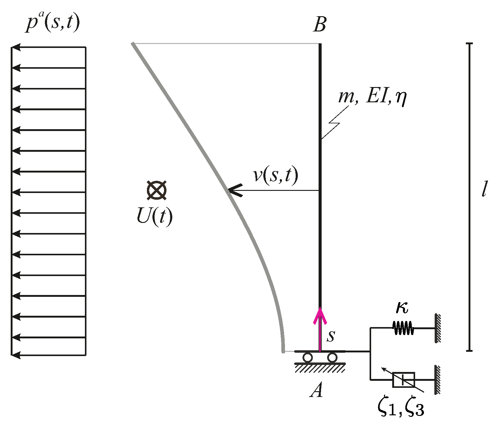
2.1. Nonlinear Aeroelastic Model

The aeroelastic behavior of a base-isolated tall building, with a square cross-section and subjected to a turbulent wind flow, is investigated. The system is similar to the one proposed in [37], but here the structural model, besides the aerodynamic one, is assumed to be nonlinear as well. The building is modeled by a planar visco-elastic Euler-Bernoulli beam (Figure 1), obeying the Kelvin-Voigt constitutive law. The beam is free at the top, and constrained at ground by a visco-elastic device, consisting of a rheological model made of a linear elastic spring of stiffness $\kappa$ in-parallel with a nonlinear dashpot. This last is characterized by a linear viscosity coefficient ${\zeta }_1$ and a nonlinear (van der Pol-like) viscosity coefficient ${\zeta }_3$. The wind velocity $U\left(t\right)$ is assumed to be uniform in space and equal to:

$$U\left(t\right)=\overline{U}+\widehat{u}cos\mathsf{\Omega }t$$

(1)

in which $\overline{U}$ is the (leading) steady-state wind velocity, and $\widehat{u}(\ll \overline{U})$ the amplitude and $\mathsf{\Omega }$ the fundamental frequency of the turbulent component (the higher harmonics being neglected). The flow induces aerodynamic loads $p_a\left(s,t\right)$ nonlinearly depending on the structural velocity $\dot{v}\left(s,t\right)$, described by the quasi-steady theory [44].

The relevant equations of motion and boundary conditions are derived in Appendix A, extending those obtained in [45] to the case of Kelvin-Voigt material and base isolation. Introduction of the following positions is done:

$$\begin{array}{cccccccccc}\hfill v^{*}& ≔ \frac{v}{l},\hfill & \hfill s^{*}& ≔ \frac{s}{l},\hfill & \hfill t^{*}& ≔ t{\omega }_r,\hfill & \hfill {\mathsf{\Omega }}^{*}& ≔ \frac{\mathsf{\Omega }}{{\omega }_r},\hfill & \hfill {\omega }_r& ≔ \frac{1}{l^2}\sqrt{\frac{EI}{m}},\hfill \\ \hfill {\eta }^{*}& ≔ \eta {\omega }_r,\hfill & \hfill c_e^{*}& ≔ c_e\frac{{\omega }_r{l}^4}{EI},\hfill & \hfill b_i^{*}& ≔ b_i\frac{{\omega }_r^2{l}^5}{EI},\hfill & \hfill {\overline{U}}^{*}& ≔ \frac{\overline{U}}{{\omega }_{r}l},\hfill & \hfill {\widehat{u}}^{*}& ≔ \frac{\widehat{u}}{{\omega }_{r}l},\hfill \\ \hfill {\kappa }^{*}& ≔ \kappa \frac{l^3}{EI},\hfill & \hfill {\zeta }_1^{*}& ≔ {\zeta }_1\frac{l^3{\omega }_r}{EI},\hfill & \hfill {\zeta }_3^{*}& ≔ {\zeta }_3\frac{l^5{\omega }_r}{EI}\hfill \end{array}$$

(2)

where $v\left(s,t\right)$ is the transverse displacement at the abscissa $s\in \left[0,l\right]$ and time $t\in \left[0,\infty \right)$, with l the length of the beam; $EI$ is the flexural stiffness of the beam; m is the mass per unit length; $\eta$ is the internal viscous damping coefficient; $c_e$ is the external damping coefficient, accounting for dissipation of the beam in motionless air; $b_i≔ {\displaystyle \frac{1}{2}}{\varrho }_{a}D{A}_i$ (for $i=1,3$) where ${\varrho }_a$ is the air mass density and $A_i$ are dimensionless aerodynamic coefficients, depending on the cross-section shape, of which D is a characteristic length; ${\omega }_r$ is a reference frequency; prime and dot denote differentiation with respect to the non-dimensional abscissa and time, respectively.

Accounting for Equation (2) and omitting the asterisks, the nondimensional form of the partial differential equation is found to be:

$$\begin{array}{cc}\hfill \ddot{v}& +(c_e+b_1\overline{U})\dot{v}+{[v^{″}\left(1+\frac{v^{\prime 2}}{2}\right)+\eta {\left[v^{″}\left(1+\frac{v^{\prime 2}}{2}\right)\right]}^{•}]}^{″}+{\left[{(v^{″}+\eta {\dot{v}}^{″})}^{\prime }\frac{v^{\prime 2}}{2}\right]}^{\prime }\hfill \\ & +\frac{v^{\prime }}{2}{\left[{\displaystyle {{\displaystyle \int }}_0^s}{v}^{\prime 2}\left(\xi \right)d\xi \right]}^{••}+\frac{v^{″}}{2}{{\displaystyle \int }}_1^s{\left[{\displaystyle {{\displaystyle \int }}_0^{\xi }}{v}^{\prime 2}\left(\xi \right)d\xi \right]}^{••}d\xi \hfill \\ & +\frac{b_3}{\overline{U}}{\dot{v}}^3+\left(b_1\dot{v}-\frac{b_3}{{\overline{U}}^2}{\dot{v}}^3\right)\widehat{u}\cos \left(\mathsf{\Omega }t\right)=0\hfill \end{array}$$

(3)

with boundary conditions:

$$\begin{array}{cc}& v_A^{\prime }=0\hfill \\ & {[v_A^{″}\left(1+\frac{v_A^{\prime 2}}{2}\right)+\eta {\left[v_A^{″}\left(1+\frac{v_A^{\prime 2}}{2}\right)\right]}^{•}]}^{\prime }+\left(v_A^{‴}+\eta {\dot{v}}_A^{‴}\right)\frac{v_A^{\prime 2}}{2}\hfill \\ & +\kappa v_A+{\zeta }_1{\dot{v}}_A+{\zeta }_3{\dot{v}}_A{v}_A^2=0\hfill \\ & -{[v_B^{″}\left(1+\frac{v_B^{\prime 2}}{2}\right)+\eta {\left[v_B^{″}\left(1+\frac{v_B^{\prime 2}}{2}\right)\right]}^{•}]}^{\prime }-\left(v_B^{‴}+\eta {\dot{v}}_B^{‴}\right)\frac{v_B^{\prime 2}}{2}=0\hfill \\ & v_B^{″}\left(1+\frac{v_B^{\prime 2}}{2}\right)+\eta {\left[v_B^{″}\left(1+\frac{v_B^{\prime 2}}{2}\right)\right]}^{•}+\left(v_B^{″}+\eta {\dot{v}}_B^{″}\right)\frac{v_B^{\prime 2}}{2}\hfill \end{array}$$

(4)

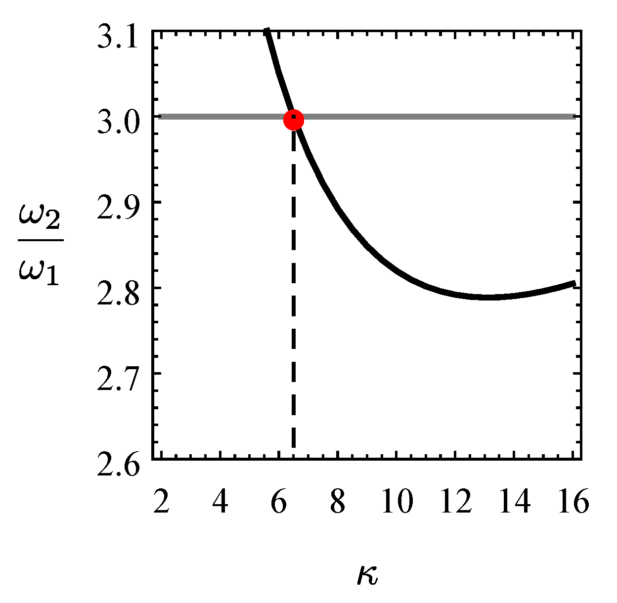
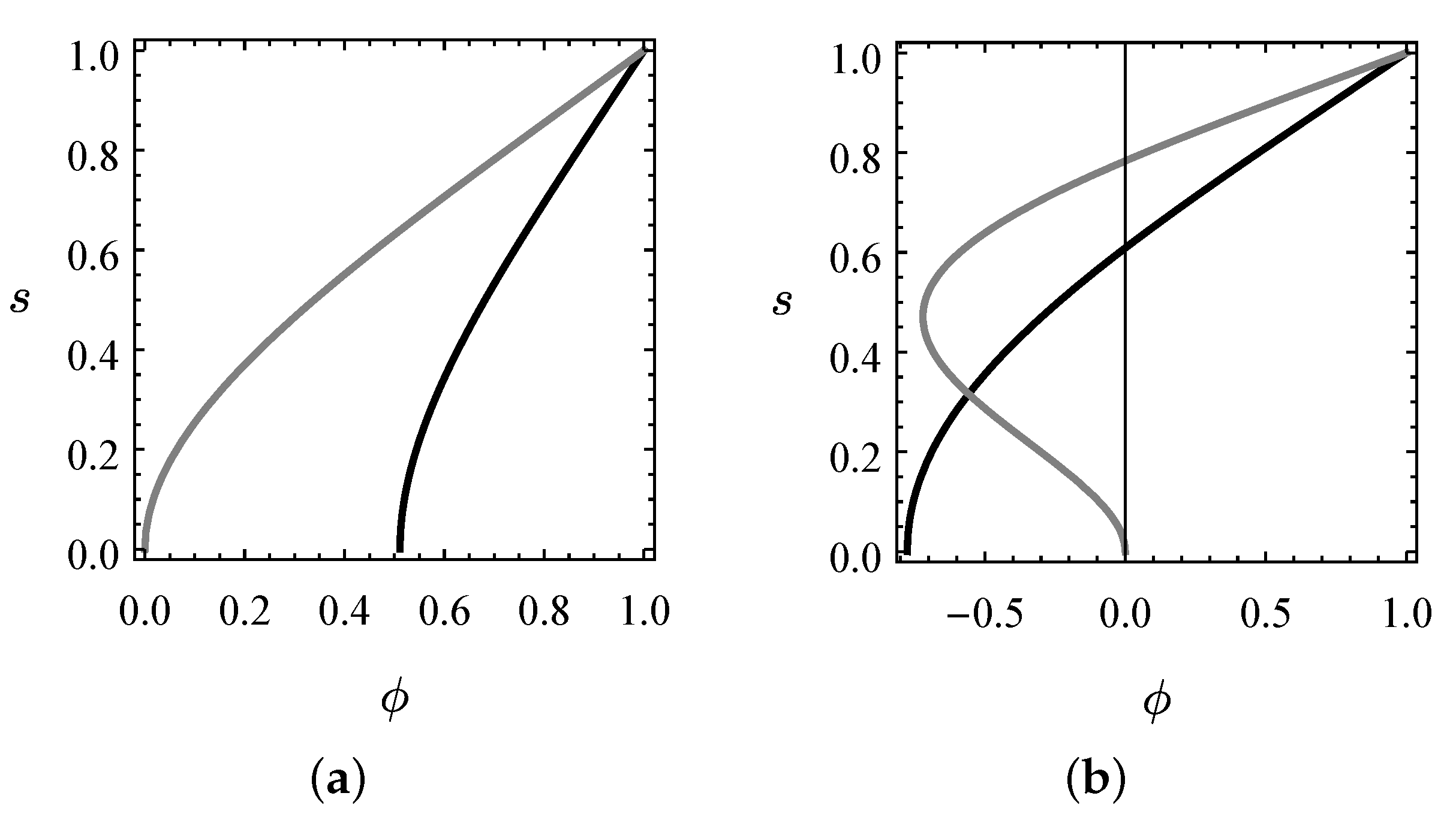
2.2. Modal Proprieties

First, free dynamics of the undamped and unloaded beam, constrained at ground by the elastic spring $\kappa$, are addressed, to evaluate the natural frequencies and modes. To this aim, by letting $v\left(s,t\right)=\phi \left(s\right)e^{i\omega t}$ and substituting it in Equations (3) and (4), the following boundary value problem is derived, when retaining linear terms and neglecting structural and aerodynamic damping:

$$\begin{array}{cc}\hfill & {\phi }^{″″}-{\omega }^2\phi =0\hfill \\ \hfill & {\phi }_A^{\prime }=0\hfill \\ \hfill & {\phi }_A^{‴}+\kappa {\phi }_A=0\hfill \\ \hfill -& {\phi }_B^{‴}=0\hfill \\ \hfill & {\phi }_B^{″}=0\hfill \end{array}$$

(5)

with $\left(\omega ,\phi \left(s\right)\right)$ a real eigenpair. The solution reads:

$$\phi \left(s\right)=c_{1}sin\left(\alpha s\right)+c_{2}cos\left(\alpha s\right)+c_{3}sinh\left(\alpha s\right)+c_{4}cosh\left(\alpha s\right)$$

(6)

with $\alpha ≔ \sqrt{\omega }$ a root of the transcendental characteristic equation:

$$\frac{{\alpha }^{3}tan\left(\alpha \right)}{\kappa }+\frac{{\alpha }^{3}tanh\left(\alpha \right)}{\kappa }=sec\left(\alpha \right)\sec \mathrm{h}\left(\alpha \right)+1$$

(7)

The system natural frequencies, therefore, depend on the stiffness $\kappa$ of the base elastic spring. Aimed to investigate possible internal resonances, the ratio ${\omega }_2/{\omega }_1$ between the second and the first root of Equation (7) is evaluated by varying the stiffness $\kappa$, see Figure 2. It is observed that, for $\kappa =6.5$, a 1:3 internal resonance occurs.

The relevant frequencies ${\omega }_1$ and ${\omega }_2$ of the two first natural modes, and the coefficients of the associated modal shapes ${\phi }_1\left(s\right)$ and ${\phi }_2\left(s\right)$, normalized according to $\phi \left(1\right)=1$, are reported in

Table 1. Frequencies and coefficients of the natural modes 1 and 2 of both uncontrolled and controlled system; the modes are normalized according to $\phi \left(1\right)=1$. Internally resonant case for $\kappa =6.5$.

	Uncontrolled (U)			Controlled (C)
	Mode 1	Mode 2		Mode 1	Mode 2
$\omega$	3.52	22.03		2.17	6.51
$c_1$	0.37	−0.51		0.52	−0.15
$c_2$	−0.50	0.50		−0.17	−0.70
$c_3$	−0.37	0.51		−0.52	0.15
$c_4$	0.50	0.50		0.68	−0.07

, for both the uncontrolled ($\kappa \to \infty$) and controlled ($\kappa =6.5$) systems. The modal shapes are also shown in Figure 3. They show that the chosen spring stiffness allows quite large (but again acceptable) displacements at the base, according which the isolation system is effective (in the linear field). Therefore, this particular internally resonant case deserves to be analyzed.

3. Perturbation Analysis

The perturbation analysis is carried out here to evaluate the bifurcation equations and analyze in detail the post-critical solutions, into a small region of the parameter space. It is performed using the Multiple Scale Method in direct approach [46], i.e., directly applying the method to the PDE of motion (3) and (4), on the same line followed in [37], where a 1:2 resonance between the first mode of the beam and the turbulence excitation term is considered. However, here the procedure is extended to the concurrent 1:3 internal resonance condition between the first two modes of the beam, and taking into account the structural nonlinear contributions as well.

Introducing a small and positive bookkeeping parameter $ϵ$, the following scaling of variable is chosen:

$$v={ϵ}^{1/2}\widehat{v}$$

(8)

consistently with systems with cubic nonlinear terms; for the parameters, the scaling is:

$$\begin{array}{cccccccccccc}\hfill & c_e=ϵ{\widehat{c}}_e,\hfill & \hfill & \eta =ϵ\widehat{\eta },\hfill & \hfill & b_1=ϵ{\widehat{b}}_1,\hfill & \hfill & {\zeta }_1=ϵ{\widehat{\zeta }}_1,\hfill & \hfill & {\zeta }_3=O\left(1\right),\hfill & & b_3=O\left(1\right)\end{array}$$

(9)

which brings linear damping and wind effect to the highest perturbation order here considered.

Time scales are introduced, as $t_0=t$, $t_1=ϵt$, and time-derivatives consistently become:

$$\frac{\partial }{\partial t}={\partial }_0+ϵ{\partial }_1,\frac{{\partial }^2}{\partial t^2}={\partial }_0^2+2ϵ{\partial }_0{\partial }_1$$

(10)

where ${\partial }_j=\frac{\partial }{\partial t_j}$, $j=0,1$. Moreover, series expansion of the dependent variable is applied:

$$\widehat{v}={\widehat{v}}_0+ϵ{\widehat{v}}_1$$

(11)

Resonance conditions read:

$$\begin{array}{c}\hfill \mathsf{\Omega }=2{\omega }_1+ϵ{\sigma }_e\\ \hfill {\omega }_2=3{\omega }_1+ϵ{\sigma }_i\end{array}$$

(12)

where ${\sigma }_e,{\sigma }_i$ are the external and internal detuning parameters, respectively.

Substituting Equations (8)–(11) in Equations (3) and (4), dividing by ${ϵ}^{1/2}$ and collecting terms multiplying ${ϵ}^0$ and ${ϵ}^1$, respectively, the following perturbation equations are obtained (omitting hat):

$$\begin{array}{cc}\hfill & \begin{array}{cc}\hfill & {\partial }_0^2{v}_0+v_0^{″″}=0\hfill \end{array}\hfill \\ \hfill & \left.\begin{array}{cc}\hfill & v_0^{\prime }=0\hfill \\ \hfill & v_0^{‴}+\kappa v_0=0\hfill \end{array}\right\}\mathrm{at}s=0\hfill \\ \hfill & \left.\begin{array}{cc}\hfill -& v_0^{‴}=0\hfill \\ \hfill & v_0^{″}=0\hfill \end{array}\right\}\mathrm{at}s=1\hfill \end{array}$$

(13)

and

$$\begin{array}{cc}\hfill & \begin{array}{cc}\hfill & {\partial }_0^2{v}_1+v_1^{″″}=-2{\partial }_0{\partial }_1{v}_0-{\left[v_0^{\prime }{\left(v_0^{\prime }{v}_0^{″}\right)}^{\prime }\right]}^{\prime }-\eta {\partial }_0{v}_0^{″″}-\frac{v_0^{\prime }}{2}{\partial }_0^2\left[{\int }_0^s{v}_0^{\prime 2}\left(\xi \right)d\xi \right]\hfill \\ \hfill & -\frac{v_0^{″}}{2}{\int }_1^s{\partial }_0^2\left[{\int }_0^{\xi }{v}_0^{\prime 2}\left(\zeta \right)d\zeta \right]d\xi -(c_e+b_{1}U){\partial }_0{v}_0-\frac{b_3}{U}{\left({\partial }_0{v}_0\right)}^3\hfill \\ \hfill & -\left(b_{1}U{\partial }_0{v}_0-\frac{b_3}{U^2}{\left({\partial }_0{v}_0\right)}^3\right)\widehat{u}cos\left(\mathsf{\Omega }t\right)\hfill \end{array}\hfill \\ \hfill & \left.\begin{array}{cc}\hfill v_1^{\prime }& =0\hfill \\ \hfill v_1^{‴}& +\kappa v_1=-v_0^{\prime }{\left(v_0^{\prime }{v}_0^{″}\right)}^{\prime }-\eta {\partial }_0{v}_0^{‴}-{\zeta }_1{\partial }_0{v}_0-{\zeta }_3{\partial }_0{v}_0{v}_0^2\hfill \end{array}\right\}\mathrm{at}s=0\hfill \\ \hfill & \left.\begin{array}{cc}\hfill -v_1^{‴}& =v_0^{\prime }{\left(v_0^{\prime }{v}_0^{″}\right)}^{\prime }+\eta {\partial }_0{v}_0^{‴}\hfill \\ \hfill v_1^{″}& =-v_0^{\prime 2}{v}_0^{″}-\eta {\partial }_0{v}_0^{″}\hfill \end{array}\right\}\mathrm{at}s=1\hfill \end{array}$$

(14)

Equation (13) provides the generating solution:

$$v_0=A_1\left(t_1\right)e^{i{\omega }_1{t}_0}{\phi }_1\left(s\right)+A_2\left(t_1\right)e^{i{\omega }_2{t}_0}{\phi }_2\left(s\right)+\mathrm{c}.\mathrm{c}.$$

(15)

where, due to the presence of damping, only internally resonant modes are retained, with $A_1\left(t_1\right),A_2\left(t_1\right)$ slow time varying complex amplitudes to be determined, c.c. standing for complex conjugate and i for the imaginary unit. Substitution of Equation (15) in Equation (14), with use of Equation (12), provides:

$$\begin{array}{cc}\hfill & \begin{array}{cc}\hfill & v_1^{″″}-{\partial }_0^2{v}_1=q_1(s,t_1)e^{i{\omega }_1{t}_0}+q_2(s,t_1)e^{i{\omega }_2{t}_0}+\mathrm{N}.\mathrm{R}.\mathrm{T}\hfill \end{array}\hfill \\ \hfill & \left.\begin{array}{cc}\hfill & v_1^{\prime }=0\hfill \\ \hfill & v_1^{‴}+\kappa v_1=Q_1(0,t_1)e^{i{\omega }_1{t}_0}+Q_2(0,t_1)e^{i{\omega }_2{t}_0}+\mathrm{N}.\mathrm{R}.\mathrm{T}\hfill \end{array}\right\}\mathrm{at}s=0\hfill \\ \hfill & \left.\begin{array}{cc}\hfill -& v_1^{‴}=Q_1(1,t_1)e^{i{\omega }_1{t}_0}+Q_2(1,t_1)e^{i{\omega }_1{t}_0}+\mathrm{N}.\mathrm{R}.\mathrm{T}\hfill \\ \hfill & v_1^{″}=C_1(1,t_1)e^{i{\omega }_1{t}_0}+C_2(1,t_1)e^{i{\omega }_1{t}_0}+\mathrm{N}.\mathrm{R}.\mathrm{T}\hfill \end{array}\right\}\mathrm{at}s=1\hfill \end{array}$$

(16)

where $q_j,Q_j,C_j$, $j=1,2$, having the meaning of distributed loads, point-forces and couples, respectively, collect resonant terms and N.R.T. stands for non-resonant terms. For the sake of brevity, definition of $q_j,Q_j,C_j$ is omitted here.

Solvability conditions must be imposed in order to remove resonant terms at the right hand side of Equation (16). It assumes the form of the Virtual Power Equation, namely:

$$\begin{array}{cc}\hfill & {\int }_0^1{q}_1(s,t_1){\phi }_1\left(s\right)ds+Q_1(0,t_1){\phi }_1\left(0\right)+Q_1(1,t_1){\phi }_1\left(1\right)+C_1(1,t_1){\phi }_1^{\prime }\left(1\right)=0\hfill \\ \hfill & {\int }_0^1{q}_2(s,t_1){\phi }_2\left(s\right)ds+Q_2(0,t_1){\phi }_2\left(0\right)+Q_2(1,t_1){\phi }_2\left(1\right)+C_2(1,t_1){\phi }_2^{\prime }\left(1\right)=0\hfill \end{array}$$

(17)

Coming back to the time t and reabsorbing $ϵ$, Equation (17) produces the following Amplitude Modulation Equations (AME):

$$\begin{array}{cc}\hfill {\dot{A}}_1& =\left(d_{10}+\overline{U}{\widehat{d}}_{10}\right)A_1+\left(\frac{d_2}{\overline{U}}+{\widehat{d}}_2+i{\tilde{d}}_2\right)A_1^2{\overline{A}}_1+\widehat{u}\frac{d_1}{\overline{U}}{A}_1^3{e}^{-it{\sigma }_e}+\widehat{u}{d}_{11}{A}_2{e}^{it\left({\sigma }_i-{\sigma }_e\right)}\hfill \\ \hfill & +\widehat{u}{d}_{12}{\overline{A}}_1{e}^{it{\sigma }_e}+\widehat{u}\frac{d_3}{\overline{U}}{A}_1{A}_2{\overline{A}}_1{e}^{it\left({\sigma }_i-{\sigma }_e\right)}+\widehat{u}\frac{d_4}{\overline{U}}{A}_1{\overline{A}}_1^2{e}^{it{\sigma }_e}\hfill \\ \hfill & +\left(\frac{d_5}{\overline{U}}+{\widehat{d}}_5+i{\tilde{d}}_5\right)A_2{\overline{A}}_1^2{e}^{it{\sigma }_i}+\widehat{u}\frac{d_6}{\overline{U}}{A}_1^2{\overline{A}}_2{e}^{it\left({\sigma }_e-{\sigma }_i\right)}\hfill \\ \hfill & +\left(\frac{d_7}{\overline{U}}+{\widehat{d}}_7+i{\tilde{d}}_7\right)A_1{A}_2{\overline{A}}_2+\widehat{u}\frac{d_8}{\overline{U}}{A}_2^2{\overline{A}}_2{e}^{it\left({\sigma }_i-{\sigma }_e\right)}\hfill \\ \hfill & +\widehat{u}\frac{d_9}{\overline{U}}{A}_2{\overline{A}}_1{\overline{A}}_2{e}^{it{\sigma }_e}\hfill \\ \hfill {\dot{A}}_2& =\left(d_{22}+\overline{U}{\widehat{d}}_{22}\right)A_2+\widehat{u}{d}_{21}{A}_1{e}^{it\left({\sigma }_e-{\sigma }_i\right)}+\left(\frac{d_{13}}{\overline{U}}+{\widehat{d}}_{13}+i{\tilde{d}}_{13}\right)A_1^3{e}^{-it{\sigma }_i}\hfill \\ \hfill & +\widehat{u}\frac{d_{14}}{\overline{U}}{A}_1^2{A}_2{e}^{-it{\sigma }_e}+\widehat{u}\frac{d_{15}}{\overline{U}}{A}_1^2{\overline{A}}_1{e}^{it\left({\sigma }_e-{\sigma }_i\right)}+\left(\frac{d_{16}}{\overline{U}}+{\widehat{d}}_{16}+i{\tilde{d}}_{16}\right)A_1{A}_2{\overline{A}}_1\hfill \\ \hfill & +\widehat{u}\frac{d_{17}}{\overline{U}}{A}_2^2{\overline{A}}_1{e}^{it\left({\sigma }_i-{\sigma }_e\right)}+\widehat{u}\frac{d_{18}}{\overline{U}}{A}_2{\overline{A}}_1^2{e}^{it{\sigma }_e}\hfill \\ \hfill & +\widehat{u}\frac{d_{19}}{\overline{U}}{A}_1{A}_2{\overline{A}}_2{e}^{it\left({\sigma }_e-{\sigma }_i\right)}+\left(\frac{d_{20}}{\overline{U}}+{\widehat{d}}_{20}+i{\tilde{d}}_{20}\right)A_2^2{\overline{A}}_2\hfill \end{array}$$

(18)

where the coefficients are given in Appendix B. It is worth noting that the structural geometric and inertial nonlinear terms give rise to the coefficients indicated as ${\tilde{d}}_j$, $j=2,5,7,13,16,20$, which contribute as imaginary parts of the relevant terms.

The real form of the AME is obtained using the polar transformation, namely $A_1\left(t\right)=\frac{a_1\left(t\right)}{2}{e}^{i{\vartheta }_1\left(t\right)}$ and $A_2\left(t\right)=\frac{a_2\left(t\right)}{2}{e}^{i{\vartheta }_2\left(t\right)}$, to be substituted in Equation (18). Then, separating real and imaginary parts and defining the phase differences ${\psi }_1\left(t\right)=2{\vartheta }_1\left(t\right)-{\sigma }_{e}t$ and ${\psi }_2\left(t\right)={\vartheta }_2\left(t\right)-3{\vartheta }_1\left(t\right)+{\sigma }_{i}t$, the real AME become:

$$\begin{array}{cc}\hfill {\dot{a}}_1& =\left(d_{10}+\overline{U}{\widehat{d}}_{10}\right)a_1+\widehat{u}{d}_{12}cos{\psi }_1{a}_1+\frac{1}{4}\widehat{u}\frac{d_1}{\overline{U}}cos{\psi }_1{a}_1^3+\frac{1}{4}\left(\frac{d_2}{\overline{U}}+{\widehat{d}}_2\right)a_1^3+\frac{1}{4}\widehat{u}\frac{d_4}{\overline{U}}cos{\psi }_1{a}_1^3\hfill \\ \hfill & +\widehat{u}{d}_{11}cos\left({\psi }_1+{\psi }_2\right)a_2+\frac{1}{4}\widehat{u}\frac{d_3}{\overline{U}}cos\left({\psi }_1+{\psi }_2\right)a_1^2{a}_2+\frac{1}{4}\left(\left(\frac{d_5}{\overline{U}}+{\widehat{d}}_5\right)cos{\psi }_2-{\tilde{d}}_{5}sin{\psi }_2\right)a_1^2{a}_2\hfill \\ \hfill & +\frac{1}{4}\widehat{u}cos\left({\psi }_1+{\psi }_2\right)\frac{d_6}{\overline{U}}{a}_1^2{a}_2+\frac{1}{4}\left(\frac{d_7}{\overline{U}}+{\widehat{d}}_7\right)a_1{a}_2^2+\frac{1}{4}\widehat{u}\frac{d_9}{\overline{U}}cos{\psi }_1{a}_1{a}_2^2+\frac{1}{4}\widehat{u}\frac{d_8}{\overline{U}}cos\left({\psi }_1+{\psi }_2\right)a_2^3\hfill \\ \hfill {\dot{a}}_2& =\widehat{u}{d}_{21}cos\left({\psi }_1+{\psi }_2\right)a_1+\frac{1}{4}\left(\left(\frac{d_{13}}{\overline{U}}+{\widehat{d}}_{13}\right)cos{\psi }_2+{\tilde{d}}_{13}sin{\psi }_2\right)a_1^3+\frac{1}{4}\widehat{u}\frac{d_{15}}{\overline{U}}cos\left({\psi }_1+{\psi }_2\right)a_1^3\hfill \\ \hfill & +\left(d_{22}+\overline{U}{\widehat{d}}_{22}\right)a_2+\frac{1}{4}\widehat{u}\frac{d_{14}}{\overline{U}}cos{\psi }_1{a}_1^2{a}_2+\frac{1}{4}\left(\frac{d_{16}}{\overline{U}}+{\widehat{d}}_{16}\right)a_1^2{a}_2+\frac{1}{4}\widehat{u}\frac{d_{18}}{\overline{U}}cos{\psi }_1{a}_1^2{a}_2\hfill \\ \hfill & +\frac{1}{4}\widehat{u}\frac{d_{17}}{\overline{U}}cos\left({\psi }_1+{\psi }_2\right)a_1{a}_2^2+\frac{1}{4}\widehat{u}\frac{d_{19}}{\overline{U}}cos\left({\psi }_1+{\psi }_2\right)a_1{a}_2^2+\frac{1}{4}\left(\frac{d_{20}}{\overline{U}}+{\widehat{d}}_{20}\right)a_2^3\hfill \\ \hfill a_1{\dot{\psi }}_1& =-{\sigma }_e{a}_1-2\widehat{u}{d}_{12}sin{\psi }_1{a}_1+\frac{1}{2}\widehat{u}\frac{d_1}{\overline{U}}sin{\psi }_1{a}_1^3-\frac{1}{2}\widehat{u}\frac{d_4}{\overline{U}}sin{\psi }_1{a}_1^3+2\widehat{u}{d}_{11}sin\left({\psi }_1+{\psi }_2\right)a_2\hfill \\ \hfill & +\frac{1}{2}\left(\left(\frac{d_5}{\overline{U}}+{\widehat{d}}_5\right)sin{\psi }_2+{\tilde{d}}_{5}cos{\psi }_2\right)a_1^2{a}_2+\frac{1}{2}\widehat{u}\frac{d_3}{\overline{U}}sin\left({\psi }_1+{\psi }_2\right)a_1^2{a}_2\hfill \\ \hfill & -\frac{1}{2}\widehat{u}\frac{d_6}{\overline{U}}sin\left({\psi }_1+{\psi }_2\right)a_1^2{a}_2-\frac{1}{2}\widehat{u}\frac{d_9}{\overline{U}}sin{\psi }_1{a}_1{a}_2^2+\frac{1}{2}\widehat{u}\frac{d_8}{\overline{U}}sin\left({\psi }_1+{\psi }_2\right)a_2^3+\frac{1}{2}{\tilde{d}}_2{a}_1^3+\frac{1}{2}{\tilde{d}}_7{a}_1{a}_2^2\hfill \\ \hfill a_1{a}_2{\dot{\psi }}_2& =-\widehat{u}{d}_{21}sin\left({\psi }_1+{\psi }_2\right)a_1^2-\frac{1}{4}\left(\left(\frac{d_{13}}{\overline{U}}+{\widehat{d}}_{13}\right)sin{\psi }_2-{\tilde{d}}_{13}sin{\psi }_2\right)a_1^4-\frac{1}{4}\widehat{u}\frac{d_{15}}{\overline{U}}sin\left({\psi }_1+{\psi }_2\right)a_1^4\hfill \\ \hfill & +{\sigma }_i{a}_1{a}_2+3\widehat{u}{d}_{12}sin{\psi }_1{a}_1{a}_2-\frac{3}{4}\widehat{u}\frac{d_1}{\overline{U}}sin{\psi }_1{a}_1^3{a}_2+\frac{3}{4}\widehat{u}\frac{d_4}{\overline{U}}sin{\psi }_1{a}_1^3{a}_2+\frac{1}{4}\widehat{u}\frac{d_{14}}{\overline{U}}sin{\psi }_1{a}_1^3{a}_2\hfill \\ \hfill & -\frac{1}{4}\widehat{u}\frac{d_{18}}{\overline{U}}sin{\psi }_1{a}_1^3{a}_2-3\widehat{u}{d}_{11}sin\left({\psi }_1+{\psi }_2\right)a_2^2-\frac{3}{4}\left(\left(\frac{d_5}{\overline{U}}+{\widehat{d}}_5\right)sin{\psi }_2+{\tilde{d}}_{5}cos{\psi }_2\right)a_1^2{a}_2^2\hfill \\ \hfill & -\frac{3}{4}\widehat{u}\frac{d_3}{\overline{U}}sin\left({\psi }_1+{\psi }_2\right)a_1^2{a}_2^2+\frac{3}{4}\widehat{u}\frac{d_6}{\overline{U}}sin\left({\psi }_1+{\psi }_2\right)a_1^2{a}_2^2+\frac{1}{4}\widehat{u}\frac{d_{17}}{\overline{U}}sin\left({\psi }_1+{\psi }_2\right)a_1^2{a}_2^2\hfill \\ \hfill & -\frac{1}{4}\widehat{u}\frac{d_{19}}{\overline{U}}sin\left({\psi }_1+{\psi }_2\right)a_1^2{a}_2^2+\frac{3}{4}\widehat{u}\frac{d_9}{\overline{U}}sin{\psi }_1{a}_1{a}_2^3-\frac{3}{4}\widehat{u}\frac{d_8}{\overline{U}}sin\left({\psi }_1+{\psi }_2\right)a_2^4\hfill \\ \hfill & -\frac{1}{4}\left(3{\tilde{d}}_2-{\tilde{d}}_{16}\right)a_1^3{a}_2+\frac{1}{4}{\tilde{d}}_{16}{a}_1^3-\frac{1}{4}\left(3{\tilde{d}}_7-{\tilde{d}}_{20}\right)a_1{a}_2^2\hfill \end{array}$$

(19)

Equilibrium solutions are sought imposing ${\dot{a}}_1={\dot{a}}_2={\dot{\psi }}_1={\dot{\psi }}_2=0$ in Equation (19), and their stability is evaluated through the sign of the real part of the eigenvalues of the Jacobian matrix of the same system. More specifically, to evaluate the stability of the trivial solution, the Cartesian form of Equation (18) is evaluated as well, after substituting $A_1\left(t\right)=(p_1\left(t\right)+i{q}_1\left(t\right))exp(it{\sigma }_e/2)$, $A_2\left(t\right)=(p_2\left(t\right)+i{q}_2\left(t\right))exp\left(it(3{\sigma }_e/2-{\sigma }_i)\right)$ and separating real and imaginary parts. Consequently, the Jacobian matrix evaluated at the trivial solution reads:

$$J_c=\left(\begin{array}{cccc}{d}_{10}+\overline{U}{\widehat{d}}_{10}+\widehat{u}{d}_{12}& \frac{{\sigma }_e}{2}& \widehat{u}{d}_{11}& 0\\ -\frac{{\sigma }_e}{2}& d_{10}+\overline{U}{\widehat{d}}_{10}-\widehat{u}{d}_{12}& 0& \widehat{u}{d}_{11}\\ \widehat{u}{d}_{21}& 0& d_{22}& \frac{3}{2}{\sigma }_e-{\sigma }_i\\ 0& \widehat{u}{d}_{21}& -\frac{3}{2}{\sigma }_e+{\sigma }_i& d_{22}\end{array}\right)$$

(20)

and the changes in sign of the real parts of its eigenvalues are sought applying the Hurwitz criterion [47] to the characteristic polynomial $det(J_c-\lambda I)=0$, where I is the identity matrix of dimension 4. It is worth noting that the number of bifurcation parameters to perform a complete unfolding of system (19) is four (e.g., $(\overline{U},\widehat{u},{\sigma }_e,{\sigma }_i)$), which corresponds to its codimension.

The expression of the beam displacement $v(s,t)$ is reconstituted through Equation (15), which becomes:

$$\begin{array}{cc}\hfill v(s,t)& =a_1\left(t\right)cos\left(\frac{\mathsf{\Omega }}{2}t+\frac{{\psi }_1\left(t\right)}{2}\right){\phi }_1\left(s\right)+a_2\left(t\right)cos\left(\frac{3}{2}\mathsf{\Omega }t+\frac{3}{2}{\psi }_1\left(t\right)+{\psi }_2\left(t\right)\right){\phi }_2\left(s\right)\hfill \end{array}$$

(21)

where Equation (12) is used. From Equation (21), equilibra of Equation (19) correspond to periodic evolution of the displacement of the beam points, whereas periodic solutions in terms of amplitudes $a_1,a_2$ give rise to quasi-periodic evolution of the beam.

Numerical calculations and parameter-continuation of the solutions of Equation (19), as well as bifurcation and stability analysis, are carried out within the software AUTO [48], combined with integration of the same equations in Mathematica [49].

4. Numerical Results

The complete unfolding of the codimension-four bifurcation is out of the scope of this paper. Here, however, the turbulence amplitude is kept fixed to the value $\widehat{u}=0.1$, whereas, for different values of the internal detuning ${\sigma }_i$, the critical and post-critical behavior is analyzed on the plane $({\sigma }_e,\overline{U})$. More specifically, the values ${\sigma }_i=0$, i.e., perfect internal resonance, and ${\sigma }_i=-0.06$, i.e., slightly far from the internal resonance, are alternatively considered, in order to assess the transition from a resonant to non-resonant case [50]. The other system parameters assume the following values: $\kappa =6.5$, $\eta =0.00026$, $c_e=0.025$, $b_1=-0.046$, $b_3=0.384$, ${\zeta }_1=0.02$.

Different configurations of the viscous-elastic device are also addressed, namely the case of linear controlled beam (LC), i.e., ${\zeta }_3=0$, to be compared to the outcomes of the nonlinear controlled system (NLC), where ${\zeta }_3=50$. A further comparison with the uncontrolled (UC) case, realized when the base is fixed ($\kappa \to +\infty$), is carried out as well. In the above mentioned cases, geometric and inertia nonlinear contributions are not considered (${\tilde{d}}_j$ set to zero), in order to be consistent with the model proposed in [37], where nonlinearities come from aerodynamic and viscous device only and where, however, exclusively the first mode was considered (NLC-1M). Finally, the effect of structural geometric and inertial nonlinear contributions is addressed (NLC-NL), through the modification produced by the coefficients ${\tilde{d}}_j$ to the NLC case. The considered cases are summarized in

Table 2. Summary of the analyzed cases.

Case	Control Device	Geometry and Inertia	Number of Modes
UC	No (Fixed base)	Linear	2
LC	Linear	Linear	2
NLC	Nonlinear	Linear	2
NLC-1M [37]	Nonlinear	Linear	1
NLC-NL	Nonlinear	Nonlinear	2

.

First, the stability domain of the trivial solution $(a_1,a_2)=(0,0)$ is shown in Figure 4 for the uncontrolled and controlled cases, where only the first bifurcations are reported. The plots are in good agreement with those reported in [37] since, due to the nature of the considered damping, always the first mode is directly involved in the bifurcation, being the second one pulled along (as it will be confirmed later). For the same reason, the domains turn out to be insensitive to ${\sigma }_i$, however, in dependence on ${\sigma }_e$, the first bifurcation is of Hopf type (H, for $|{\sigma }_e|<0.0022$) or of Neimark type (N, for $|{\sigma }_e|\ge 0.0022$). For $|{\sigma }_e|<0.0022$, second Hopf bifurcations are found as well (SH, upper semi-perimeter of the ellipses). The control through the viscous-elastic device (black lines) generally induces an increasing of the critical values of $\overline{U}$, as expected, whereas the nonlinear terms in the equations do not affect the domains, they being ruled only by the linear ones.

In Figure 5, the bifurcation diagrams for amplitudes $a_1,a_2$ as functions of $\overline{U}$ are shown, obtained as vertical path in Figure 4 for ${\sigma }_e=0$. In particular, solid and dashed lines represent stable and unstable equilibria, respectively, whereas the filled regions indicate limit cycles in the amplitudes $a_1,a_2$, the former corresponding to (stable and unstable) periodic motions of the beam and the latter to quasi-periodic evolution. Comparison between controlled and uncontrolled (grey line, UC) cases shows that the control system pushes forward the first and second Hopf bifurcation points. Specifically, from the first point a stable branch arises, whereas from the second one the branch is unstable. Moreover, the NLC case (red line) shows smaller amplitudes in the post-critical evolution than the LC case (black line). If only one mode is considered (NLC-1M, blue line), a similar behavior to NLC is found for $a_1$. Considering the nonlinear geometric and inertia terms (NLC-NL, orange line) modifies very slightly the amplitudes of the post-critical branches compared to the NLC case, except for their nature: periodic motions occur up to $\overline{U}=1.27$; then, for increasing $\overline{U}$, quasi-periodic solutions are found, even if their modulation amplitudes are small. As a final comments, amplitude $a_1$ is one order of magnitude larger than $a_2$ and the bifurcated branch arises perpendicularly to the trivial one for $a_1$, whereas it presents horizontal tangent for $a_2$, as a confirmation of the pulling along of the second mode by the first one.

The combined 3D bifurcation diagram, relevant to the case NCL-NL only, is shown in Figure 6, where it is evident the initial tangency of the bifurcated branch to the $(\overline{U},a_2)$ plane, as it is found also in other internally resonant problems [51].

For the same values of parameters, and for $\overline{U}=1.25$, the phase plots of the reconstituted displacement (Equation (21)) of the beam, at cross-section $s=0.5$ and $s=1$, respectively, are shown in Figure 7. It is confirmed the reduction of the limit cycle amplitude due to the nonlinear control device. Moreover, slight differences appear between NLC-NL and: (i) NLC, where structural geometric and inertial nonlinearities are neglected; (ii) NLC-1M, where the second mode is ignored.

When ${\sigma }_e=0.003$ is considered, the bifurcation diagram for amplitudes $a_1,a_2$ as functions of $\overline{U}$ are shown in Figure 8. The major difference with respect to the perfect resonant case of Figure 5 is related to the different kind of bifurcation point, which is on Neimark type. Indeed, filled regions indicate that quasi-periodic solutions arise, however with modulation amplitudes which appear quite small. Furthermore, periodic motions are found for the UC and LC cases for larger values of $\overline{U}$, in some regions even coexisting with quasi-periodic evolution (LC).

Quite far from internal resonance, Figure 9 shows the bifurcation diagram for amplitudes $a_1,a_2$ as functions of $\overline{U}$ at ${\sigma }_i=-0.06$, and for ${\sigma }_e=0$. There, for better visibility, quasi-periodic solutions are omitted, whereas only periodic motion branches are shown. The behavior is qualitatively similar to the corresponding internally resonant case (Figure 5), even if smaller amplitudes $a_2$ occur here, due to the weaker nonlinear interaction between the two modes.

As final comments, the efficiency of the nonlinear control device is confirmed, both in pushing forward the bifurcation and in reduction of the post-critical amplitudes. The internal resonance for the analyzed cases appears as a weak phenomenon compared to the galloping induced on the first mode, slightly modifying the post-critical evolution with the presence of the minor component $a_2$. Nonlinear structural geometry and inertia give minor contributions as well, confirming the almost linear features of cantilevers [52], even in the case of internal resonance.

5. Conclusions

The aeroelastic behavior of a tall building modeled as an Euler-Bernoulli beam is considered here. Base isolation with a nonlinear viscous-elastic device is assumed, for vibration mitigation purpose. The steady component of the wind triggers galloping, whereas the turbulent component, with harmonic evolution, is in principal parametric resonance with the first mode of the beam. Internal resonance in ratio 1:3 between the first and second beam mode, reached after suitable calibration of the base device, is considered as well.

After the application of the Multiple Scale Method in direct approach, a bifurcation analysis is carried out to evaluate the effects of the nonlinear viscous term of the device, the internal resonance and the structural nonlinear geometric and inertial terms.

The main conclusions can be summarized as follows:

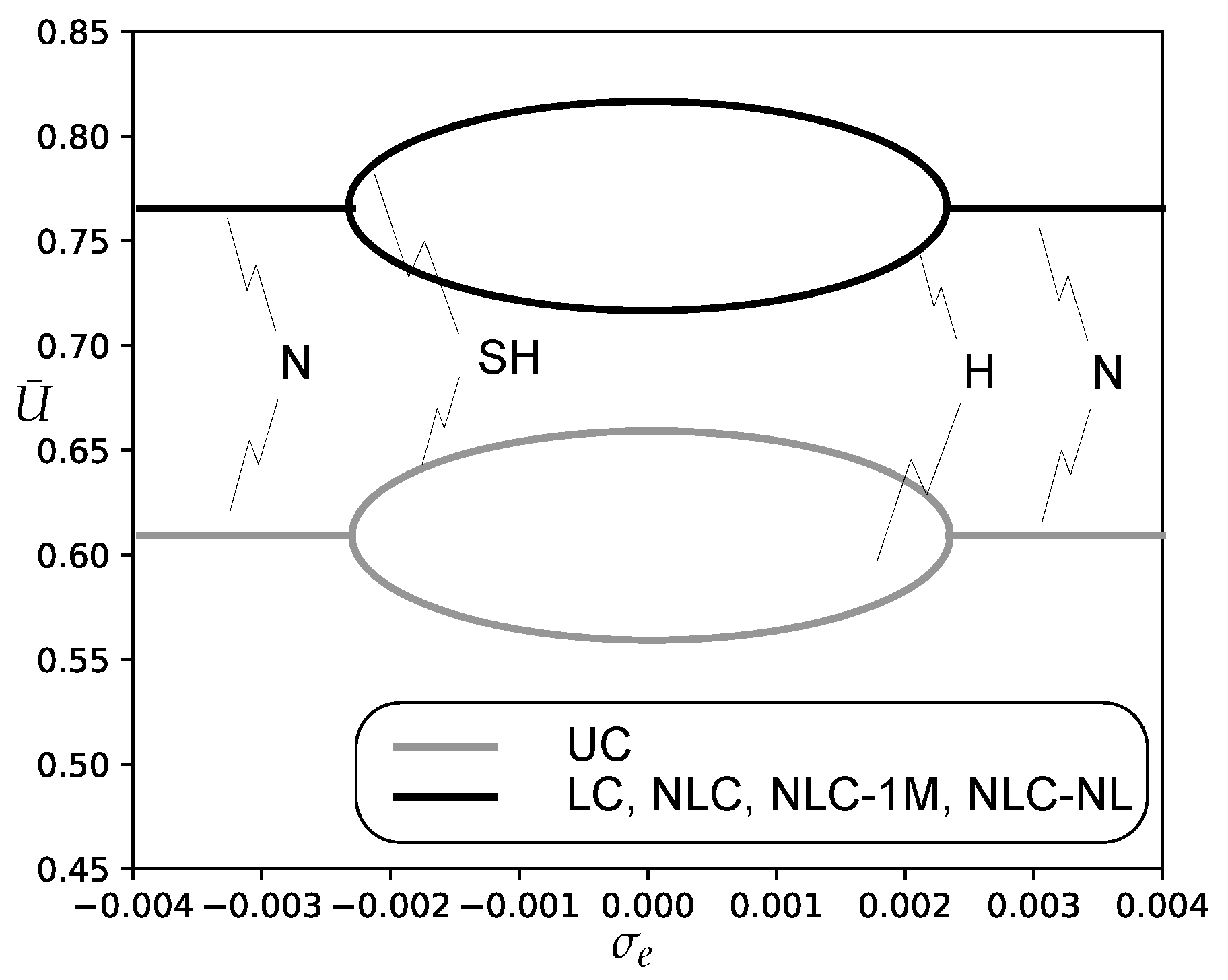
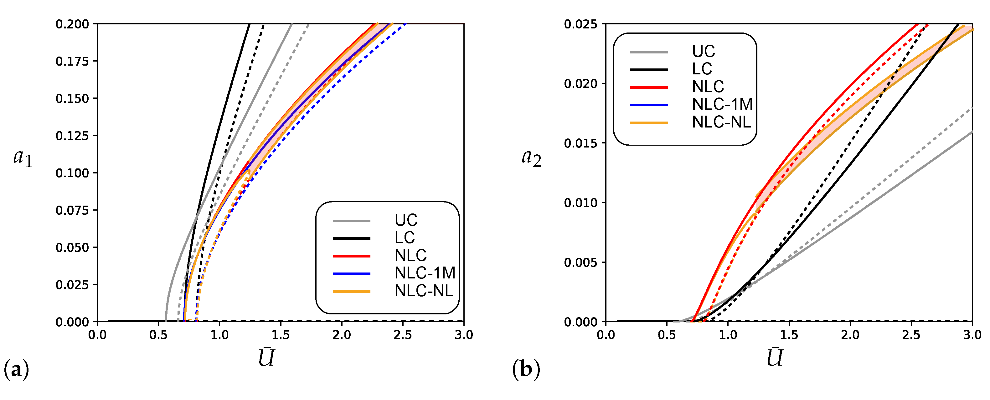
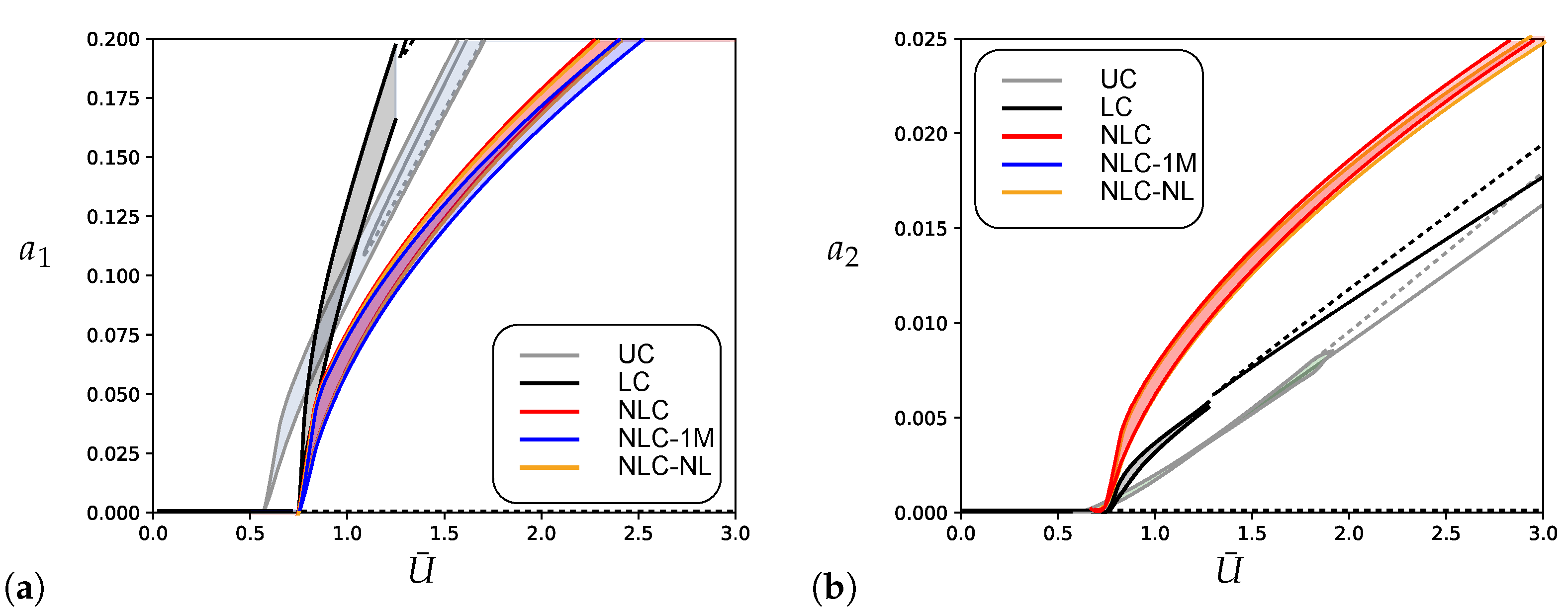
• The base device, through its linear viscous component, pushes forward the bifurcation point, as expected;
• The nonlinear viscous term of the device reduces the amplitude of the post-critical evolution, as compared to the use of a purely linear device;
• The galloping induced by the mean wind on the first mode represents the leading phenomenon, being the second mode marginally involved in the motion due to its smaller amplitudes;
• The structural nonlinearities provide weak modification to the response, confirming the almost linear behavior of the cantilever, even when internal resonance occurs.

References

1. Tang, D.; Dowell, E.H. Experimental and theoretical study on aeroelastic response of high-aspect-ratio wings. AIAA J. 2001, 39, 1430–1441. [Google Scholar] [CrossRef]
2. Afonso, F.; Vale, J.; Oliveira, É.; Lau, F.; Suleman, A. A review on non-linear aeroelasticity of high aspect-ratio wings. Prog. Aerosp. Sci. 2017, 89, 40–57. [Google Scholar] [CrossRef]
3. Riziotis, V.; Voutsinas, S.; Politis, E.; Chaviaropoulos, P. Aeroelastic stability of wind turbines: The problem, the methods and the issues. Wind. Energy Int. J. Prog. Appl. Wind. Power Convers. Technol. 2004, 7, 373–392. [Google Scholar] [CrossRef]
4. Hansen, M.H. Aeroelastic instability problems for wind turbines. Wind. Energy Int. J. Prog. Appl. Wind. Power Convers. Technol. 2007, 10, 551–577. [Google Scholar] [CrossRef]
5. Tokoro, S.; Komatsu, H.; Nakasu, M.; Mizuguchi, K.; Kasuga, A. A study on wake-galloping employing full aeroelastic twin cable model. J. Wind. Eng. Ind. Aerodyn. 2000, 88, 247–261. [Google Scholar] [CrossRef]
6. Luongo, A.; Zulli, D. Dynamic instability of inclined cables under combined wind flow and support motion. Nonlinear Dyn. 2012, 67, 71–87. [Google Scholar] [CrossRef]
7. Ferretti, M.; Zulli, D.; Luongo, A. A continuum approach to the nonlinear in-plane galloping of shallow flexible cables. Adv. Math. Phys. 2019, 2019, 6865730. [Google Scholar] [CrossRef] [Green Version]
8. Larsen, A. Advances in aeroelastic analyses of suspension and cable-stayed bridges. J. Wind. Eng. Ind. Aerodyn. 1998, 74, 73–90. [Google Scholar] [CrossRef]
9. Diana, G.; Rocchi, D.; Argentini, T.; Muggiasca, S. Aerodynamic instability of a bridge deck section model: Linear and nonlinear approach to force modeling. J. Wind. Eng. Ind. Aerodyn. 2010, 98, 363–374. [Google Scholar] [CrossRef]
10. Di Nino, S.; Luongo, A. Nonlinear Aeroelastic in-Plane Behavior of Suspension Bridges under Steady Wind Flow. Appl. Sci. 2020, 10, 1689. [Google Scholar] [CrossRef] [Green Version]
11. Kawai, H. Effect of corner modifications on aeroelastic instabilities of tall buildings. J. Wind. Eng. Ind. Aerodyn. 1998, 74, 719–729. [Google Scholar] [CrossRef]
12. Braun, A.L.; Awruch, A.M. Aerodynamic and aeroelastic analyses on the CAARC standard tall building model using numerical simulation. Comput. Struct. 2009, 87, 564–581. [Google Scholar] [CrossRef]
13. Cluni, F.; Gioffrè, M.; Gusella, V. Dynamic response of tall buildings to wind loads by reduced order equivalent shear-beam models. J. Wind. Eng. Ind. Aerodyn. 2013, 123, 339–348. [Google Scholar] [CrossRef]
14. Piccardo, G.; Tubino, F.; Luongo, A. A shear-shear torsional beam model for nonlinear aeroelastic analysis of tower buildings. Z. Angew. Math. Phys. 2015, 66, 1895–1913. [Google Scholar] [CrossRef]
15. Piccardo, G.; Tubino, F.; Luongo, A. Equivalent nonlinear beam model for the 3-D analysis of shear-type buildings: Application to aeroelastic instability. Int. J. Non-Linear Mech. 2016, 80, 52–65. [Google Scholar] [CrossRef]
16. Zulli, D.; Luongo, A. Nonlinear dynamics and stability of a homogeneous model of tall buildings under resonant action. J. Appl. Comput. Mech. 2020. [Google Scholar] [CrossRef]
17. Lu, O.; To, C. Principal resonance of a nonlinear system with two-frequency parametric and self-excitations. Nonlinear Dyn. 1991, 2, 419–444. [Google Scholar] [CrossRef]
18. Szabelski, K.; Warmiński, J. Parametric self-excited non-linear system vibrations analysis with inertial excitation. Int. J. Non-Linear Mech. 1995, 30, 179–189. [Google Scholar] [CrossRef]
19. El-Bassiouny, A. Principal parametric resonances of non-linear mechanical system with two-frequency and self-excitations. Mech. Res. Commun. 2005, 32, 337–350. [Google Scholar] [CrossRef]
20. Di Nino, S.; Luongo, A. Nonlinear interaction between self-and parametrically excited wind-induced vibrations. Nonlinear Dyn. 2021, 103, 79–101. [Google Scholar] [CrossRef]
21. Abdel-Rohman, M. Effect of unsteady wind flow on galloping of tall prismatic structures. Nonlinear Dyn. 2001, 26, 233–254. [Google Scholar] [CrossRef]
22. Luongo, A.; Zulli, D. Parametric, external and self-excitation of a tower under turbulent wind flow. J. Sound Vib. 2011, 330, 3057–3069. [Google Scholar] [CrossRef] [Green Version]
23. Zulli, D.; Luongo, A. Bifurcation and stability of a two-tower system under wind-induced parametric, external and self-excitation. J. Sound Vib. 2012, 331, 365–383. [Google Scholar] [CrossRef] [Green Version]
24. Zulli, D.; Di Egidio, A. Galloping of internally resonant towers subjected to turbulent wind. Contin. Mech. Thermodyn. 2015, 27, 835–849. [Google Scholar] [CrossRef]
25. Kirrou, I.; Mokni, L.; Belhaq, M. On the quasiperiodic galloping of a wind-excited tower. J. Sound Vib. 2013, 332, 4059–4066. [Google Scholar] [CrossRef]
26. Belhaq, M.; Kirrou, I.; Mokni, L. Periodic and quasiperiodic galloping of a wind-excited tower under external excitation. Nonlinear Dyn. 2013, 74, 849–867. [Google Scholar] [CrossRef]
27. Bottasso, C.L.; Croce, A.; Gualdoni, F.; Montinari, P. Load mitigation for wind turbines by a passive aeroelastic device. J. Wind. Eng. Ind. Aerodyn. 2016, 148, 57–69. [Google Scholar] [CrossRef] [Green Version]
28. Graham, J.M.R.; Limebeer, D.J.; Zhao, X. Aeroelastic control of long-span suspension bridges. J. Appl. Mech. 2011, 78, 041018. [Google Scholar] [CrossRef]
29. Ribeiro, L.P.; de Lima, A.M.G. Robust passive control methodology and aeroelastic behavior of composite panels with multimodal shunted piezoceramics in parallel. Compos. Struct. 2020, 262, 113348. [Google Scholar] [CrossRef]
30. Lee, Y.S.; Vakakis, A.F.; Bergman, L.A.; McFarland, D.M.; Kerschen, G. Suppression aeroelastic instability using broadband passive targeted energy transfers, part 1: Theory. AIAA J. 2007, 45, 693–711. [Google Scholar] [CrossRef]
31. Lee, Y.S.; Kerschen, G.; McFarland, D.M.; Hill, W.J.; Nichkawde, C.; Strganac, T.W.; Bergman, L.A.; Vakakis, A.F. Suppressing aeroelastic instability using broadband passive targeted energy transfers, part 2: Experiments. AIAA J. 2007, 45, 2391–2400. [Google Scholar] [CrossRef]
32. Gendelman, O.V.; Vakakis, A.F.; Bergman, L.A.; McFarland, D.M. Asymptotic analysis of passive nonlinear suppression of aeroelastic instabilities of a rigid wing in subsonic flow. SIAM J. Appl. Math. 2010, 70, 1655–1677. [Google Scholar] [CrossRef]
33. Vaurigaud, B.; Manevitch, L.I.; Lamarque, C.H. Passive control of aeroelastic instability in a long span bridge model prone to coupled flutter using targeted energy transfer. J. Sound Vib. 2011, 330, 2580–2595. [Google Scholar] [CrossRef]
34. Luongo, A.; Zulli, D. Aeroelastic instability analysis of NES-controlled systems via a mixed multiple scale/harmonic balance method. J. Vib. Control 2014, 20, 1985–1998. [Google Scholar] [CrossRef]
35. Bichiou, Y.; Hajj, M.R.; Nayfeh, A.H. Effectiveness of a nonlinear energy sink in the control of an aeroelastic system. Nonlinear Dyn. 2016, 86, 2161–2177. [Google Scholar] [CrossRef]
36. Di Nino, S.; Luongo, A. Nonlinear aeroelastic behavior of a base-isolated beam under steady wind flow. Int. J. Non-Linear Mech. 2020, 119, 103340. [Google Scholar] [CrossRef]
37. Di Nino, S.; Luongo, A. Nonlinear dynamics of a base-isolated beam under turbulent wind flow. Nonlinear Dyn. 2021. [Google Scholar] [CrossRef]
38. Nayfeh, A.; Chin, C.; Nayfeh, S. On nonlinear normal modes of systems with internal resonance. ASME J. Vib. Acoust. 1996, 118, 340–345. [Google Scholar] [CrossRef]
39. Nayfeh, A.H.; Lacarbonara, W.; Chin, C.M. Nonlinear normal modes of buckled beams: Three-to-one and one-to-one internal resonances. Nonlinear Dyn. 1999, 18, 253–273. [Google Scholar] [CrossRef]
40. Gilliatt, H.C.; Strganac, T.W.; Kurdila, A.J. An investigation of internal resonance in aeroelastic systems. Nonlinear Dyn. 2003, 31, 1–22. [Google Scholar] [CrossRef]
41. Luongo, A.; Piccardo, G. A continuous approach to the aeroelastic stability of suspended cables in 1:2 internal resonance. J. Vib. Control 2008, 14, 135–157. [Google Scholar] [CrossRef] [Green Version]
42. Luongo, A.; Zulli, D. Nonlinear energy sink to control elastic strings: The internal resonance case. Nonlinear Dyn. 2015, 81, 425–435. [Google Scholar] [CrossRef]
43. Di Egidio, A.; Zulli, D. Critical and post-critical galloping behavior of base isolated coupled towers. Int. J. Non-Linear Mech. 2021. accepted. [Google Scholar]
44. Novak, M. Aeroelastic galloping of prismatic bodies. J. Eng. Mech. Div. 1969, 95, 115–142. [Google Scholar] [CrossRef]
45. Luongo, A.; Di Egidio, A. Bifurcation Equations Through Multiple-Scales Analysis for a Continuous Model of a Planar Beam. Nonlinear Dyn. 2005, 41, 171–190. [Google Scholar] [CrossRef] [Green Version]
46. Nayfeh, A.H.; Mook, D.T. Nonlinear Oscillations; John Wiley: New York, NY, USA, 1979. [Google Scholar]
47. Pignataro, M.; Rizzi, N.; Luongo, A. Stability, Bifurcation and Postcritical Behaviour of Elastic Structures; Elsevier: Amsterdam, The Netherlands, 1991. [Google Scholar]
48. Doedel, E.; Oldeman, B. AUTO-07P: Continuation and Bifurcation Software for Ordinary Differential Equation. 2019. Available online: http://indy.cs.concordia.ca/auto/ (accessed on 22 February 2021).
49. Wolfram Research. Mathematica, Version 12.1; Wolfram Research: Champaign, IL, USA, 2020. [Google Scholar]
50. Luongo, A.; Zulli, D. A paradigmatic system to study the transition from zero/Hopf to double-zero/Hopf bifurcation. Nonlinear Dyn. 2012, 70, 111–124. [Google Scholar] [CrossRef] [Green Version]
51. Luongo, A.; Piccardo, G. Non-Linear Galloping of Sagged Cables in 1:2 Internal Resonance. J. Sound Vib. 1998, 214, 915–940. [Google Scholar] [CrossRef] [Green Version]
52. Luongo, A.; Rega, G.; Vestroni, F. On Nonlinear Dynamics of Planar Shear Indeformable Beams. J. Appl. Mech. 1986, 53, 619–624. [Google Scholar] [CrossRef]
Figure 1. Base-isolated beam model under transverse uniform turbulent wind flow.
Applsci 11 03213 g001
Figure 2. The ratio between second and first natural frequency v s the elastic spring stiffness. Red marker denotes the internally resonant case.
Applsci 11 03213 g002
Figure 3. (a) First natural mode; (b) Second natural mode. Gray and black lines indicate the uncontrolled and controlled system, respectively. Internally resonant case for κ = 6.5 .
Applsci 11 03213 g003
Figure 4. Stability diagram of the trivial solution in the ( σ e , U ¯ ) -plane (N: Neimark bifurcation; H: Hopf bifurcation).
Applsci 11 03213 g004
Figure 5. Bifurcation diagram for σ e = 0 , σ i = 0 : (a) amplitude a 1 ; (b) amplitude a 2 (solid line: stable; dashed line: unstable).
Applsci 11 03213 g005
Figure 6. Bifurcation diagram for σ e = 0 , σ i = 0 , case NCL-NL (solid line: stable; dashed line: unstable).
Applsci 11 03213 g006
Figure 7. Phase plot for the beam for U ¯ = 1.25 , σ e = 0 , σ i = 0 : (a) at s = 0.5 ; (b) at s = 1 .
Applsci 11 03213 g007
Figure 8. Bifurcation diagram for σ e = 0.003 , σ i = 0 : (a) amplitude a 1 ; (b) amplitude a 2 (solid line: stable; dashed line: unstable).
Applsci 11 03213 g008
Figure 9. Bifurcation diagram for σ e = 0 , σ i = 0.06 : (a) amplitude a 1 ; (b) amplitude a 2 (solid line: stable; dashed line: unstable).
Applsci 11 03213 g009