Improved PR Control Strategy for an LCL Three-Phase Grid-Connected Inverter Based on Active Damping

Featured Application

The controller of a three-phase grid-connected inverter is studied and improved, which provides support for the independent control of power and the design of the controller.

Abstract

Aiming at the problem of power coupling and complicated decoupling in the d-q coordinate system of a three-phase grid-connected inverter, a current closed-loop control strategy based on an improved QPIR (quasi-proportional integral resonant) controller in the α-β two-phase static coordinate system is proposed. Firstly, the mathematical model of an LCL three-phase grid-connected inverter is established, and its instantaneous power calculation equation is deduced. Secondly, the frequency method is applied to compare and analyze the proportional resonant, quasi-proportional resonant, and improved current controller, and the appropriate improved controller parameters are obtained according to the traditional proportional integral controller parameter design method and the weight coefficient. Finally, the improved controller is compared with the traditional controller in the simulation model of the LCL three-phase grid-connected inverter based on active damping. The results show that the proposed improved current control strategy has good dynamic response characteristics, can realize the non-static error control of grid-connected current, and realizes the decoupling control of active power and reactive power when the load jumps. At the same time, the results also prove the superiority of the proposed control strategy and verify its effectiveness.

1. Introduction

High power factor and low grid-connected current total harmonic distortion are common requirements for grid-connected inverters [1,2,3]. Pulse-width modulation (PWM) technology has a wide range of applications in the field of inverters, but a grid-connected inverter using PWM control technology will produce many switching frequency subharmonics, which seriously threaten the power quality and safe operation of the power grid [4,5,6]. In order to reduce the harmonic content of the grid-connected current, an appropriate grid-connected current filter must be adopted [7,8,9]. At present, L-type and LCL-type filters are widely used in harmonic suppression of grid-connected inverter output current. Under the same capacity, an LCL filter has strong attenuation ability to high frequency interference and has a good prospect for engineering application. However, the inherent disadvantage of the low damping resonance of an LCL filter in inverter control technology is still under discussion [10,11]. Compared with the passive damping control method, active damping can provide an appropriate damping coefficient without increasing the extra loss of the system, thus achieving the purpose of weakening the resonant peak [12,13,14]. Common active damping control techniques include capacitor current feedback [15,16], capacitor voltage primary differential feedback [17], grid-connected current secondary differential feedback [18,19], and multi-state variable combined control [20,21], etc. Among them, the capacitance current proportional feedback damping effect is good, easy to realize, and the application is also the most common.

For the control method of a three-phase grid-connected inverter, the current common method is to convert it from a three-phase stationary coordinate system to a two-phase stationary coordinate system (α-β) or two-phase synchronous rotating coordinate system (d-q) [22,23,24]. In the d-q coordinate system, all control variables are DC flow, the classical PI controller can be used to realize the non-static error control of grid-connected current, and the implementation method is flexible and simple, so it has been widely used. However, there is coupling in the d-q coordinate system of the three-phase grid-connected inverter. If the active power and reactive power can be controlled independently, decoupling must be carried out. For L-type grid-connected inverters, there is only one group of coupling terms between the d axis and q axis, and the decoupling process is relatively simple. However, for LCL-type three-phase grid-connected inverters, there are three groups of coupling terms between the d axis and q axis, and the decoupling process is very complicated [25]. In practical application, due to factors such as system parameter error and interference, it is almost impossible for the inverter to achieve complete power decoupling. In the α-β coordinate system, there is no coupling term between the α axis and β axis, which creates favorable conditions for independent control of active power and reactive power. However, in the α-β coordinate system, all control quantities are AC quantities. In order to realize static error-free control, unless the gain of the controller is infinite, it is particularly important to find a controller with high gain [26,27,28].

As for the control technology of grid current in a three-phase grid-connected inverter, the commonly used control methods include proportional-integral (PI) control, proportional-resonant (PR) control, and quasi-proportional-resonant (QPR) control. The PI control structure is simple and easy to implement and is suitable for DC flow control, but the AC PI controller cannot realize non-static error control [29]. Increasing the feedforward link of the grid voltage ratio can reduce the steady-state error of grid-connected current, but cannot effectively suppress the harmonics [30]. Theoretically, the PR controller has infinite gain at the specific frequency, but the PR controller has poor adaptability to grid frequency fluctuations, so quasi-proportional resonant controllers are widely used [31,32]. The QPR controller has strong adaptability to grid frequency fluctuations, but the gain at the fundamental frequency is limited, so it can only approximately realize error-free tracking [33,34]. In addition, there are hysteresis control, repetitive control, and H_∞ control, but their control performance is not significantly better than that of PI, PR, and QPR controllers [28]. For three-phase LCL grid-connected inverters, few studies consider the steady-state error of grid-connected current and the power grid frequency fluctuation at the same time, and relevant control technologies need further research.

This paper studies the controller of the three-phase LCL grid-connected inverter in the α-β coordinate system. A current closed-loop control strategy based on an improved QPIR controller is proposed while considering the steady-state error of grid-connected current, power decoupling, and grid frequency fluctuations. Theoretical analysis and case simulation show that the QPIR controller can track the grid-connected current without static error and has good output waveform quality, which proves the correctness and effectiveness of the controller.

This paper consists of the following parts: In Section 2, the mathematical model of the LCL three-phase grid-connected inverter is established, and the advantages of independent power control in the α-β coordinate system are pointed out. In Section 3, the control method of active damping is given, and compared with the advantages and disadvantages of a traditional PR controller and QPR controller, an improved QPIR controller strategy is proposed. In Section 4, the simulation results and some discussion under different conditions are given through an LCL three-phase grid-connected inverter simulation model. The conclusion is given in Section 5.

2. Mathematical Model and Control Method

2.1. Mathematical Model of the Three-Phase LCL-Type Grid-Connected Inverter

The main circuit topology of the three-phase grid-connected inverter with the LCL filter is shown in Figure 1, wherein L₁ is the inductance on the inverter side; L₂ is the inductance on the grid side; C is a filter capacitor. The inverter supplies power to the power grid through the LCL filter. U_dc is the DC bus voltage, u_a, u_b, and u_c are the midpoint voltages of each bridge arm of the inverter, i_la, i_lb, and i_lc are the three-phase inductor currents on the inverter side, i_2a, i_2b, and i_2c are the three-phase inductor currents on the grid side, i_Ca, i_Cb, and i_Cc are the three-phase currents of the filter capacitor, u_Ca, u_Cb, and u_Cc are the three-phase voltages of the filter capacitor, u_ga, u_gb, and u_gc are the three-phase grid voltages, N is the neutral point of the LCL filter, N’ is the neutral point of the grid, and Q₁-Q₆ represent the six IGBT switch tubes of the inverter.

Assume that the three-phase grid voltage is balanced. According to Figure 1, select the inverter side inductor currents i_la, i_lb, i_lc, the grid side inductor currents i_2a, i_2b, i_2c, and the filter capacitor voltages u_Ca, u_Cb, u_Cc as state variables; the state equation in the three-phase static coordinate system can be obtained, as shown in Equation (1).

$$\{\begin{array}{l}{L}_1\frac{\mathrm{d}{i}_{1k}}{\mathrm{d}t}=u_k-u_{Ck}\\ L_2\frac{\mathrm{d}{i}_{2k}}{\mathrm{d}t}=u_{Ck}-u_{gk}\\ C\frac{\mathrm{d}{u}_{Ck}}{\mathrm{d}t}=i_{1k}-i_{2k}\end{array}\hspace{1em}\hspace{1em}k=a,b,c$$

(1)

2.2. Mathematical Model of the α-β Coordinate System

Edith Clark transformation was carried out on Equation (1) to obtain the state equation of the three-phase inverter in the two-phase stationary coordinate system, and then Laplace transformation was carried out to obtain the transfer function in the two-phase stationary coordinate system, as shown in Equations (2) and (3).

$$\{\begin{array}{l}\left[\begin{array}{l}{u}_{\alpha }\\ u_{\beta }\end{array}\right]=\left[\begin{array}{l}{u}_{C\alpha }\\ u_{C\beta }\end{array}\right]+L_{1}p\left[\begin{array}{l}{i}_{1\alpha }\\ i_{1\beta }\end{array}\right]\\ \left[\begin{array}{l}{u}_{C\alpha }\\ u_{C\beta }\end{array}\right]=\left[\begin{array}{l}{u}_{g\alpha }\\ u_{g\beta }\end{array}\right]+L_{2}p\left[\begin{array}{l}{i}_{2\alpha }\\ i_{2\beta }\end{array}\right]\\ \left[\begin{array}{l}{i}_{1\alpha }\\ i_{1\beta }\end{array}\right]=\left[\begin{array}{l}{i}_{2\alpha }\\ i_{2\beta }\end{array}\right]+Cp\left[\begin{array}{l}{u}_{C\alpha }\\ u_{C\beta }\end{array}\right]\end{array}$$

(2)

$p=\frac{\mathrm{d}}{\mathrm{d}t}$, and Laplace transformation was carried out on Equation (2) to obtain the mathematical model in the s domain, as shown in Equation (3):

$$\{\begin{array}{l}\left[\begin{array}{l}{u}_{\alpha }\\ u_{\beta }\end{array}\right]=\left[\begin{array}{l}{u}_{C\alpha }\\ u_{C\beta }\end{array}\right]+L_{1}s\left[\begin{array}{l}{i}_{1\alpha }\\ i_{1\beta }\end{array}\right]\\ \left[\begin{array}{l}{u}_{C\alpha }\\ u_{C\beta }\end{array}\right]=\left[\begin{array}{l}{u}_{g\alpha }\\ u_{g\beta }\end{array}\right]+L_{2}s\left[\begin{array}{l}{i}_{2\alpha }\\ i_{2\beta }\end{array}\right]\\ \left[\begin{array}{l}{i}_{1\alpha }\\ i_{1\beta }\end{array}\right]=\left[\begin{array}{l}{i}_{2\alpha }\\ i_{2\beta }\end{array}\right]+Cs\left[\begin{array}{l}{u}_{C\alpha }\\ u_{C\beta }\end{array}\right]\end{array}$$

(3)

As can be seen from Equation (3), there is no coupling in the two-phase static coordinate system three-phase LCL grid-connected inverter. This advantage can be fully utilized to decouple the active power and reactive power. The LCL type three-phase grid-connected inverter will be directly controlled in a two-phase stationary coordinate system.

2.3. Instantaneous Power Calculation

The calculation equation of instantaneous active power in the three-phase static coordinate system is as follows:

$$p=u_{\mathrm{a}}{i}_{\mathrm{a}}+u_b{i}_b+u_c{i}_c$$

(4)

Equivalent transformation is carried out on Equation (4):

$$\begin{gathered} p=\left[u_{\mathrm{a}}\hspace{1em}{u}_b\hspace{1em}{u}_c\right]\left[\begin{array}{l}{i}_{\mathrm{a}}\\ i_b\\ i_c\end{array}\right]=\left[u_{\mathrm{a}}\hspace{1em}{u}_b\hspace{1em}{u}_c\right]C^{-1}C\left[\begin{array}{l}{i}_{\mathrm{a}}\\ i_b\\ i_c\end{array}\right]={\left[{\left(C^{-1}\right)}^{{\rm T}}\left[\begin{array}{l}{u}_{\mathrm{a}}\\ u_b\\ u_c\end{array}\right]\right]}^{{\rm T}}\cdot C\left[\begin{array}{l}{i}_{\mathrm{a}}\\ i_b\\ i_c\end{array}\right] \\ ={\left[{\left(C^{-1}\right)}^{{\rm T}}{C}^{-1}C\left[\begin{array}{l}{u}_{\mathrm{a}}\\ u_b\\ u_c\end{array}\right]\right]}^{{\rm T}}\cdot C\left[\begin{array}{l}{i}_{\mathrm{a}}\\ i_b\\ i_c\end{array}\right] \end{gathered}$$

(5)

From the Clark transformation equation, it can be seen that:

$$\left[\begin{array}{l}{u}_{\alpha }\\ u_{\beta }\\ u_0\end{array}\right]=C\left[\begin{array}{l}{u}_{\mathrm{a}}\\ u_b\\ u_c\end{array}\right], \left[\begin{array}{l}{i}_{\alpha }\\ i_{\beta }\\ i_0\end{array}\right]=C\left[\begin{array}{l}{i}_{\mathrm{a}}\\ i_b\\ i_c\end{array}\right]$$

(6)

where the transformation matrix is:

$$C=\frac{2}{3}\left[\begin{array}{ccc}1& -\frac{1}{2}& -\frac{1}{2}\\ 0& \frac{\sqrt{3}}{2}& -\frac{\sqrt{3}}{2}\\ \frac{1}{2}& \frac{1}{2}& \frac{1}{2}\end{array}\right], C^{-1}=\left[\begin{array}{ccc}1& 0& 1\\ -\frac{1}{2}& \frac{\sqrt{3}}{2}& 1\\ -\frac{1}{2}& -\frac{\sqrt{3}}{2}& 1\end{array}\right]$$

By inserting Equation (5) and Equation (6) into Equation (4), we can obtain:

$$p=\left[u_{\alpha }\hspace{1em}{u}_{\beta }\hspace{1em}{u}_0\right]{\left(C^{-1}\right)}^{{\rm T}}{C}^{-1}\left[\begin{array}{l}{i}_{\alpha }\\ i_{\beta }\\ i_0\end{array}\right]$$

(7)

Through further calculation, the expression of instantaneous active power in two-phase stationary coordinate system is as follows:

$$p=\frac{3}{2}(u_{\alpha }{i}_{\alpha }+u_{\beta }{i}_{\beta }+2u_0{i}_0)$$

(8)

Similarly, according to the above calculation method of active power, the expression of instantaneous reactive power can be obtained as follows:

$$q=\frac{3}{2}(u_{\beta }{i}_{\alpha }-u_{\alpha }{i}_{\beta })$$

(9)

With the above instantaneous power expression, the grid-connected inverter can be controlled by the power outer loop.

3. Analysis of the Control Strategy

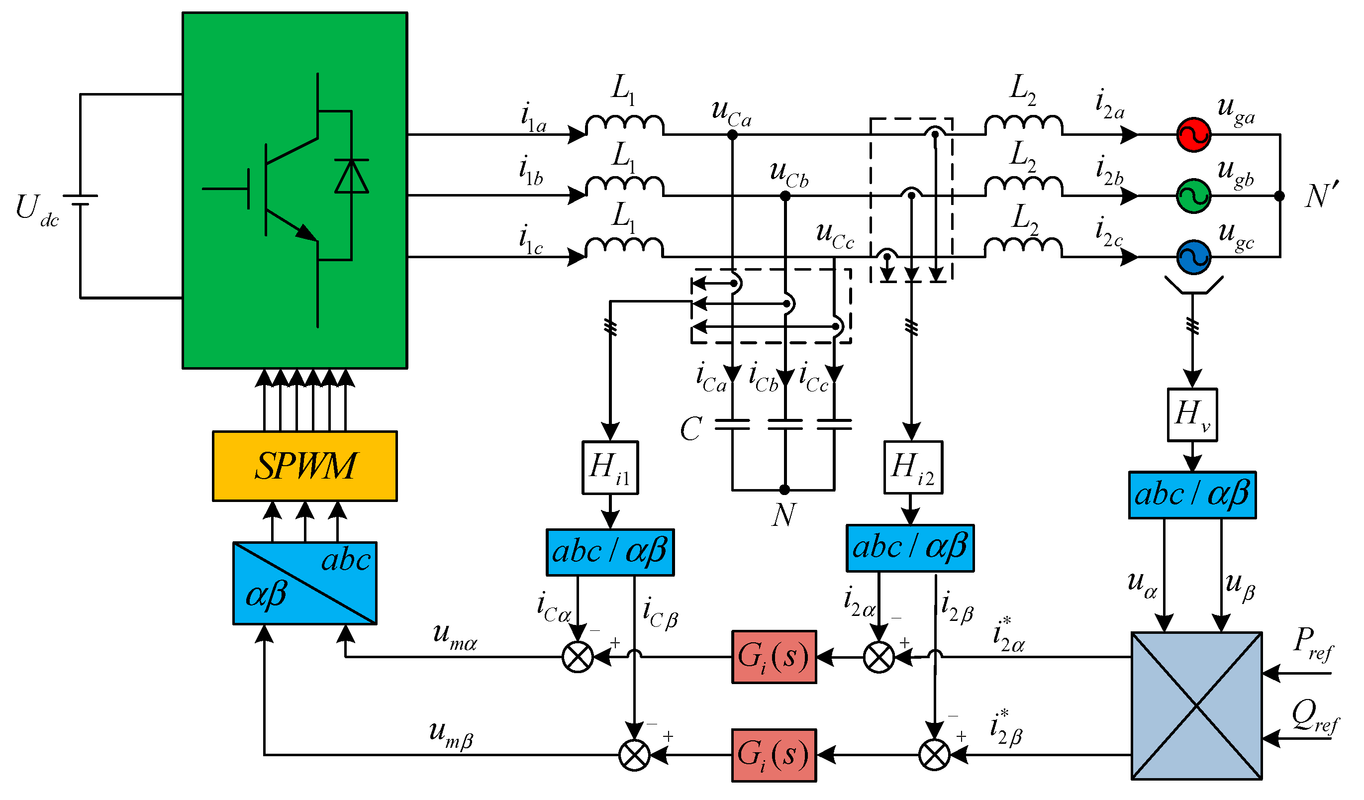
3.1. LCL-Type Three-Phase Grid-Connected Inverter Control Structure

The control structure diagram of the LCL-type grid-connected inverter is shown in Figure 2. After collecting the voltage and current of the three-phase power grid from the external large power grid, through Edith Clark transformation, u_α, u_β and i_α, i_β are obtained. According to the instantaneous power calculation principle, the current reference values i_2α^* and i_2β^* of the current loop can be obtained and then compared with the grid-connected feedback currents i_2α and i_2β. After the error signal is adjusted by the improved G_QPIR(s) controller, the PWM controller controls the on and off status of the switch tube.

According to Equation (3) and considering the control system structure given in Figure 2, the s domain model of the three-phase LCL grid-connected inverter controlled in the α-β coordinate system can be obtained, as shown in Figure 3. K_PWM is the transfer function of the voltage-source three-phase inverter bridge modulated by PWM, and H_i1 and H_i2 are the capacitance current feedback coefficient and grid-connected current feedback coefficient, respectively.

3.2. Capacitor Current Feedback Active Damping

Capacitor current feedback active damping will not reduce the low-frequency gain and high-frequency harmonic attenuation capability of the LCL filter and will not increase the additional power loss of the system, thus having very good practical value [14].

See Appendix A for the capacitor current proportional feedback active damping parameters. Figure 4 is a Bode diagram of loop gain T(s) after active damping with capacitor current feedback, where f₀ is the fundamental frequency, f_c is the cutoff frequency, and f_r is the resonant frequency. As can be seen from Figure 4, the introduction of capacitor current feedback can weaken the resonant peak of the LCL filter. With the increase in damping coefficient H_i1, the damping effect of the resonant peak will be better, and at the same time it will not affect the low frequency and high frequency characteristics of the system.

3.3. Performance Comparison of the PR and QPR Controller

In the current control of the grid-connected inverter in a α-β coordinate system, the PR controller can obtain higher gain at the fundamental wave of the power grid or a specific frequency and can eliminate the steady-state error of the grid-connected current or inhibit the influence of a specific subharmonic on the grid-connected current. The QPR controller has good robustness and adaptability to power grid frequency fluctuation. The following is a comparative analysis of these two controllers.

The transfer function of the PR controller is:

$$G_{PR}(\mathrm{s})=K_1+\frac{K_2\mathrm{s}}{s^2+{\omega }_0{}^2}$$

(10)

The transfer function of the QPR controller is:

$$G_{QPR}(\mathrm{s})=K_3+\frac{K_4{\omega }_i\mathrm{s}}{s^2+2{\omega }_i\mathrm{s}+{\omega }_0{}^2}$$

(11)

K₁ and K₂ in Equations (10) and (11) are the respective proportional coefficients and resonant coefficients of the PR controller; K₃ and K₄ are the respective proportional coefficient and quasi-resonance coefficient of the QPR controller; ω₀ = 2πf₀ is the fundamental angular frequency; ω_i is the bandwidth of the resonance term considering the −3 dB requirement, i.e., the gain of the resonance term is 0.707K₄ at ω₀ ± ω_i.

Figure 5 is the Bode diagrams of G_PR(s) and G_QPR(s). For the LCL three-phase grid-connected inverter, the gain of the PR controller can obtain infinite gain at fundamental frequency, thus realizing non-static error control of the fundamental component of the grid-connected current. However, due to load changes and various interferences, the actual power grid frequency will fluctuate. When the grid frequency deviates from the fundamental frequency f₀ set by the PR controller, the gain of the PR controller will decrease rapidly, which will lead to the rapid increase in the steady-state error of the grid-connected current. The QPR controller adds parameter ω_i to the PR controller, so that it can obtain higher gain than the PR controller in a wider frequency band and can adapt to the power grid frequency fluctuation in a certain range at the same time. However, the gain at the fundamental frequency f₀ is much smaller than the gain of the PR controller, which indicates that the accuracy of the QPR controller is lower than that of the PR controller and will produce steady-state errors. Increasing the quasi-resonance coefficient K₄ can improve the gain at the fundamental frequency of the QPR controller, but due to the limitation of system stability, the value of K₄ cannot be too large.

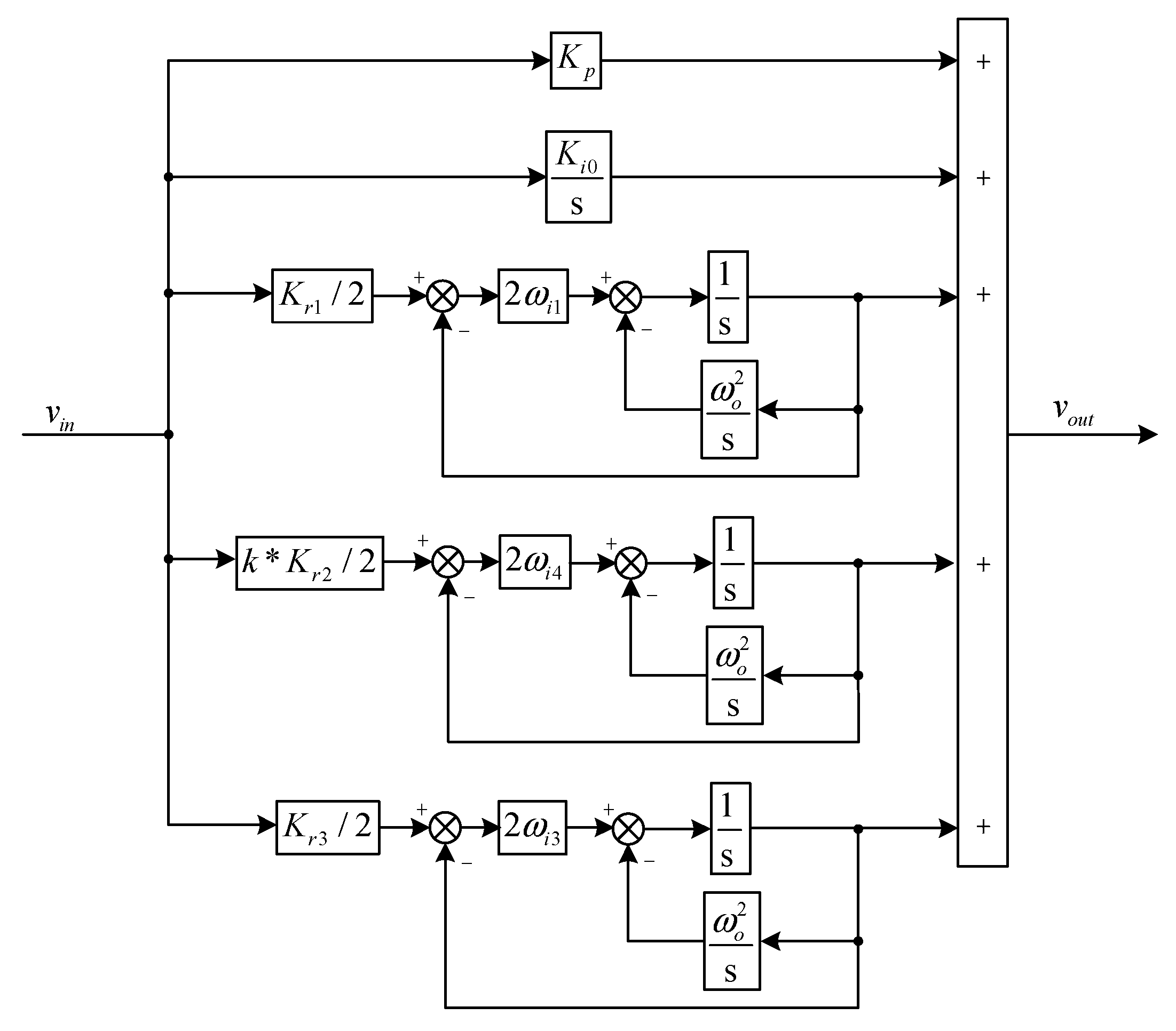
3.4. Improved Controller QPIR

As can be seen from the previous analysis, the LCL-type three-phase grid-connected inverter has no coupling in the two-phase stationary coordinate system, which creates favorable conditions for independent control of active power and reactive power. However, the control quantity in the two-phase stationary coordinate system is AC quantity, and the traditional PR and QPR controllers have their own defects, which decreases the control effect of the inverter. In order to solve this problem, this paper proposes an improved controller with proportional, integral, and quasi-resonant hybrid structures. Its transfer function is shown in Equation (12):

$$G_{QPIR}=K_P+\frac{K_{i0}}{s}+\frac{K_{r1}{\omega }_{i1}s}{s^2+2{\omega }_{i1}s+{\omega }_{o1}^2}+\frac{K_{r2}{\omega }_{i2}s}{s^2+2{\omega }_{i4}s+{\omega }_{o2}^2}+\frac{K_{r3}{\omega }_{i3}s}{s^2+2{\omega }_{i3}s+{\omega }_{o3}^2}$$

(12)

$$K_i=K_{i0}+K_{r1}{\omega }_{i1}+K_{r2}{\omega }_{i2}+K_{r3}{\omega }_{i3}=\alpha K_i+\beta K_i+\gamma K_i+\eta K_i$$

(13)

In Equations (12) and (13), K_P is the proportional coefficient, K_i0 is the integral coefficient, K_r1, K_r2, K_r3 are quasi-resonant coefficients, K_i is the total integral resonant coefficient, α, β, γ, η are the weight coefficients of K_i0, K_r1, K_r2, K_r3, respectively, ω_o1 = 2π(f₀ − Δf), ω_o2 = 2πf₀, ω_o3 = 2π(f₀ + Δf) are the fundamental angular frequencies considering the frequency fluctuation of the power grid, ω_i1, ω_i2, ω_i3, ω_i4 represent the resonant term bandwidth, and Δf is the frequency fluctuation range.

By inserting Equation (13) into Equation (12), another form can be obtained:

$$G_{QPIR}=K_P+K_i(\frac{\alpha }{s}+\frac{\beta s}{s^2+2{\omega }_{i1}s+{\omega }_{o1}^2}+\frac{\gamma s}{s^2+2{\omega }_{i4}s+{\omega }_{o2}^2}+\frac{\eta s}{s^2+2{\omega }_{i3}s+{\omega }_{o3}^2})$$

(14)

The Bode diagram of the improved controller G_QPIR(s) is shown in Figure 6. In Figure 6, the total integrated resonance coefficients of the three controllers G_PR(s), G_QPR(s), and G_QPIR(s) are all the same, but the improved controller G_QPIR(s) has different weight coefficients and resonance bandwidths. As can be seen from the Bode diagram of Figure 6, the improved QPIR controller is basically consistent with the Bode diagram of the QPR controller in other frequency bands except near the fundamental frequency. It can be seen from the local amplified Bode diagram that the Bode diagram (red) of the improved QPIR controller has a wider frequency range than the traditional PR controller (blue), and at the same time has a higher gain near the fundamental frequency compared with the traditional QPR controller (green), which can not only improve the steady-state accuracy of the grid-connected current but also has certain robustness to the fluctuation of the grid frequency.

3.5. Implementation of the QPIR Controller

In order to facilitate the realization of the QPIR controller, suppose that parameter ω_i2 is k times ω_i4 (i.e., ω_i2 = kω_i4) and the value of k is determined by the actual values of ω_i2 and ω_i4. According to Equation (12), the equivalent control block diagram can be obtained, as shown in Figure 7. The input signals of the controller pass through the proportional, integral, and quasi-proportional resonant modules, and the output signals are obtained after accumulation. For each basic module in Figure 7, we can use C language programming to achieve the output. In this way, the control strategy proposed in this paper can be implemented in the actual converter.

4. Case Analysis

In order to verify the correctness and effectiveness of the improved QPIR algorithm proposed in this paper, a system simulation model is built in MATLAB/Simulink simulation software. PR, QPR, and QPIR current controllers combined with capacitor current feedback active damping are used to simulate and compare the three-phase LCL grid-connected inverter. The system simulation parameters are shown in

Table 1. Parameters of the LCL-type three-phase grid-connected inverter system.

Project	Parameter
DC bus voltage Udc	750 V
Power grid line voltage ug (RMS)	380 V,
Rated power PN	40 kW
Inverter side inductance L1	700 μH
Network side inductance L2	110 μH
Filter capacitor C	15 μF
Fundamental frequency f0	50 Hz
Switching frequency fs	15 kHz
Capacitance current feedback coefficient Hi1	0.12
Power network current feedback coefficient Hi2	0.14
Power network voltage feedback coefficient Hv	1.00

.

It can be seen from reference [35] that when the controller parameters are the same, they also have similar performance. Therefore, in order to facilitate comparison, the QPIR controller and PR and QPR controllers are set to have similar parameters, that is, the QPIR controller parameters satisfy the following relationship:

$$K_P=K_1=K_3$$

(15)

$$K_i=K_2=K_4$$

(16)

For small photovoltaic power stations, the allowable range of grid frequency fluctuation is 49.5–50.5 Hz [36], i.e., the frequency deviation is Δf = 0.5 Hz. The system phase margin PM > 45° is selected to ensure a good dynamic response. The gain margin is GM > 3 dB for sufficient robustness. PR, QPR, and QPIR controllers are designed to meet the above conditions.

Considering the dynamic response and the attenuation of high-frequency noise, the system crossover frequency f_c usually has strict limits. Generally, f₀ << f_c << f_s, where f₀ is the fundamental frequency and f_s is the switching frequency. It can be seen from Figure 6 that when the total parameters of the controller are the same, the PR, QPR, and QPIR controllers have similar amplitude-frequency characteristic curves in the high-frequency part. In other words, for a given converter, irrespective of the controller used, the system crossover frequency is the same, so according to the system loop design requirements, set K_p = K₁ = K₄ = 0.65, K_i = K₂ω_i = K₄ω_i = 2001; for the calculation process, refer to the literature [37]. For the QPR controller, considering the fluctuation of the fundamental frequency, take the resonance bandwidth parameter ω_i = 2πΔf = π and further obtain K₆ = K_i/ω_i = 636.94. For the PR controller, further calculation can be used to obtain K₂ = 636.94.

For the QPIR controller, considering the fluctuation of the fundamental frequency, set three different fundamental angular frequencies, namely ω_o1 = 2π(f₀-Δf) = 311.02, ω_o2 = 2πf₀ = 314.16, ω_o3 = 2π(f₀ + Δf) = 317.3, making the system gain as large as possible within the frequency fluctuation range. Considering that the fluctuation of the fundamental frequency obeys a normal distribution, in order to make the controller have certain robustness, it is hoped that the bandwidth around the angular frequency ω_o2 should be larger, and the bandwidth around ω_o1 and ω_o3 should be smaller, so set the resonance bandwidth parameter ω_i1 = ω_i3 = 0.4π, ω_i2 = 2π. In order to ensure that the controller has a large gain near the fundamental frequency f₀ (49.8~50.2 Hz), it is necessary to satisfy ω_i4 < ω_i2, so that its characteristic curve is similar to that of the PR controller, and ω_i4 = 0.1 can be obtained by the estimation method. At the same time, based on the idea that the fundamental frequency is dominant and the frequency fluctuation obeys the normal distribution, the quasi-resonance coefficient of the QPIR controller is mainly allocated reasonably to make full use of its respective advantages. Take α = 1/2001, β = 300/2001, γ = 1400/2001, η = 300/2001.

Obviously, there is no coupling between the α axis and β axis in Figure 3, and there is duality. The following is an analysis of the system taking only the α axis as an example. According to the control block diagram of Figure 3, the open-loop transfer function of the system can be obtained as follows:

$$T(s)=\frac{H_{i2}{K}_{PWM}{G}_i(s)}{s^3{L}_1{L}_{2}C+s^2{L}_{2}C{H}_{i1}{K}_{PWM}+s(L_1+L_2)}$$

(17)

Figure 8 is a Bode diagram of the loop gain T(s) of different controller systems plotted according to the parameters in Table 1. In the figure, T_PR(s), T_QPR(s), and T_QPIR(s) represent the loop gain using the PR, QPR, and QPIR controllers, respectively. With the same parameters, the phase margin of the PR controllers is 67.5°, and that of the QPR and QPIR controllers is 56.1° > 45°; their amplitude margin is 4.2 dB > 3 dB, which meets the design requirements. The cutoff frequency f_c is 1756 Hz, and the resonance frequency f_r is 4125 Hz. The gain (104 dB) at the fundamental frequency f₀ with the QPIR controller is much higher than that with the QPR (76.2 dB) controller. At the same time, the QPIR controller can also meet the requirements of adapting to the power grid frequency fluctuation in the range of Δf = 0.5 Hz, similar to the QPR controller.

4.1. Analysis of Voltage and Current Based on the Improved QPIR Controller

The voltage and current waveforms, active power waveforms, and reactive power waveforms of the PR controller, QPR controller, and QPIR controller at a grid frequency of 49.5 Hz are shown in Figure 9, Figure 10 and Figure 11, respectively.

In Figure 9, when the PR controller is used, the phase error between grid-connected current and voltage is 0.09°, and the effective value of the grid-connected current is 60.26 A, which is less than the current loop reference value (60.606 A). In Figure 10 and Figure 11, P represents active power and Q represents reactive power. When the PR controller is used, the active power is 39,740 W, which is less than the given value 40 kW, and the reactive power reaches 60 var. This shows that the PR controller has errors in controlling amplitude and phase.

When the QPR controller is used, the phase error between the grid-connected current and voltage is 0.06°, and the effective value of the grid-connected current is 60.44 A, which is slightly less than the reference value. In Figure 10 and Figure 11, when the QPR controller is used, the active power is 39,870 W and the reactive power is 40 var. It is verified that the gain of the QPR controller at 49.5 Hz is not large enough to realize static error-free adjustment.

When the QPIR controller is used, the grid-connected current basically has no phase error. The effective value of the grid-connected current is 60.60 A, and the error between the grid-connected current and the reference value is basically 0. As shown in Figure 10 and Figure 11, when the QPIR controller is used, the active power approaches 40 kW and the reactive power approaches 0 var. Compared with the QPR controller, the fluctuation range of active power and reactive power is smaller. It is verified that the QPIR controller can eliminate the static error of the system, achieve the operating condition of the unit power factor, and also improve the utilization rate of DC side voltage.

The voltage and current waveforms, active power waveforms, and reactive power waveforms of the PR controller, QPR controller, and QPIR controller at a grid frequency of 50.5 Hz are shown in Figure 12, Figure 13 and Figure 14, respectively.

In Figure 12, when the PR controller is used, the phase error between the grid-connected current and voltage is 0.11°, and the effective value of the grid-connected current is 60.91 A, which is greater than the current loop reference value (60.606 A). In Figure 13 and Figure 14, P represents active power and Q represents reactive power. When the PR controller is used, the active power is 40,180 W, which is greater than the given value 40 kW, and the reactive power reaches 80 var. This shows that the PR controller has errors in controlling amplitude and phase.

When the QPR controller is used, the phase error between grid-connected current and voltage is 0.07°, and the effective value of grid-connected current is 60.8 A, which is slightly higher than the reference value. In Figure 13 and Figure 14, when the QPR controller is used, the active power is 40,110 W and the reactive power is 50 var. It is verified that the gain of the QPR controller at 50.5 Hz is not large enough to realize static error-free adjustment.

When the QPIR controller is used, the grid-connected current basically has no phase error. The effective value of the grid-connected current is 60.61 A, and the error between the grid-connected current and the reference value is basically 0. As shown in Figure 13 and Figure 14, when the QPIR controller is used, the active power approaches 40 kW and the reactive power approaches 0 var. It is verified that the QPIR controller can eliminate the static error of the system and achieve the operating condition of unit power factor.

4.2. Step Response Analysis Based on the Improved QPIR Controller

In order to verify the coupling relationship between active power and reactive power in the two-phase stationary coordinate system, the active power and reactive power jumped at 0.2 s and 0.3 s, and the power waveform is shown in Figure 15.

In Figure 15, P represents active power and Q represents reactive power. At 0.2 s, the active power suddenly jumps from 0 to full load (40 kW). It can be seen that when the active power jumps, the reactive power is hardly affected. At 0.3 s, the reactive power suddenly jumps from 0 to 40 kvar, and when the reactive power suddenly changes, the active power is hardly affected.

Figure 16 is a waveform of active power and reactive power following the reference power. At 0.2 s, when the active power reference quantity P_ref jumps, the active power output by the inverter can quickly follow the target value without overshoot. At 0.3 s, when the reactive power reference value Q_ref jumps, the reactive power output by the inverter can quickly follow the target value without overshoot.

Through the comparison between Figure 15 and Figure 16, it can be seen that there is no coupling relationship between active power and reactive power in the two-phase static coordinate system, and the improved QPIR controller can quickly follow the target value, which verifies the correctness of the previous analysis.

4.3. Frequency Fluctuation Analysis Based on the Improved QPIR Controller

Figure 17 is a chart of the power grid frequency fluctuation. A sawtooth wave is used to simulate the power grid frequency fluctuation, and the frequency fluctuation range is 49.5–50.5 Hz. Figure 18 shows power waveforms of the system using the QPIR controller and PR controller under the condition of grid frequency fluctuation according to Figure 17. Figure 19 shows power waveforms of the system using the QPIR controller and QPR controller under the condition of grid frequency fluctuation according to Figure 17.

As can be seen from the power waveform in Figure 18, when the power grid frequency fluctuates, both the QPIR controller and PR controller systems can maintain stable operation. When the power grid frequency fluctuates, the active power changes with the change in frequency, but the active power fluctuation of the QPIR controller is obviously smaller than that of the PR controller, and the reactive power is almost not affected by the frequency change. For the PR controller, the maximum deviation of active power is 300 W (at 1.2 s) and the deviation of reactive power is 45 var. For the improved QPIR controller, the maximum deviation of active power is only 75 W (at 1.2 s), and the reactive power approaches to 0. This shows that the control accuracy of the QPIR controller is significantly higher than that of the PR controller when the power grid frequency fluctuates.

As can be seen from the power waveform in Figure 19, when the power grid frequency fluctuates, the active power fluctuation of the QPIR controller is obviously smaller than that of the QPR controller, and the reactive power is almost not affected by the frequency change. For the QPR controller, the maximum deviation of active power is 200 W (at 1.2 s) and the deviation of reactive power is 50 var. For the improved QPIR controller, the maximum deviation of active power is only 75 W (at 1.2 s), and the reactive power approaches 0. This shows that the control accuracy of the QPIR controller is significantly higher than that of the QPR controller when the power grid frequency fluctuates, which verifies that the QPIR controller can adapt to the fluctuation of power grid frequency within the normal range.

The simulation results show that the steady-state control accuracy of the QPIR controller is higher than that of the PR and QPR controllers under the condition of stable power grid frequency of 49.5 Hz and 50.5 Hz. Under the condition of power grid frequency fluctuation and load variation, the steady-state control accuracy of the QPIR controller is also higher than that of the PR and QPR controllers, which has stronger adaptability to power grid frequency fluctuation and verifies the correctness and effectiveness of the theoretical analysis.

5. Conclusions

In this paper, an improved current control strategy (QPIR) for a three-phase LCL grid-connected inverter based on active damping is proposed, and the simulation and example analysis were carried out using MATLAB/Simulink software. The following conclusions were obtained:

• The LCL grid-connected inverter based on active damping can realize independent control of active power and reactive power without coupling between the α axis and β axis in a two-phase static coordinate system.
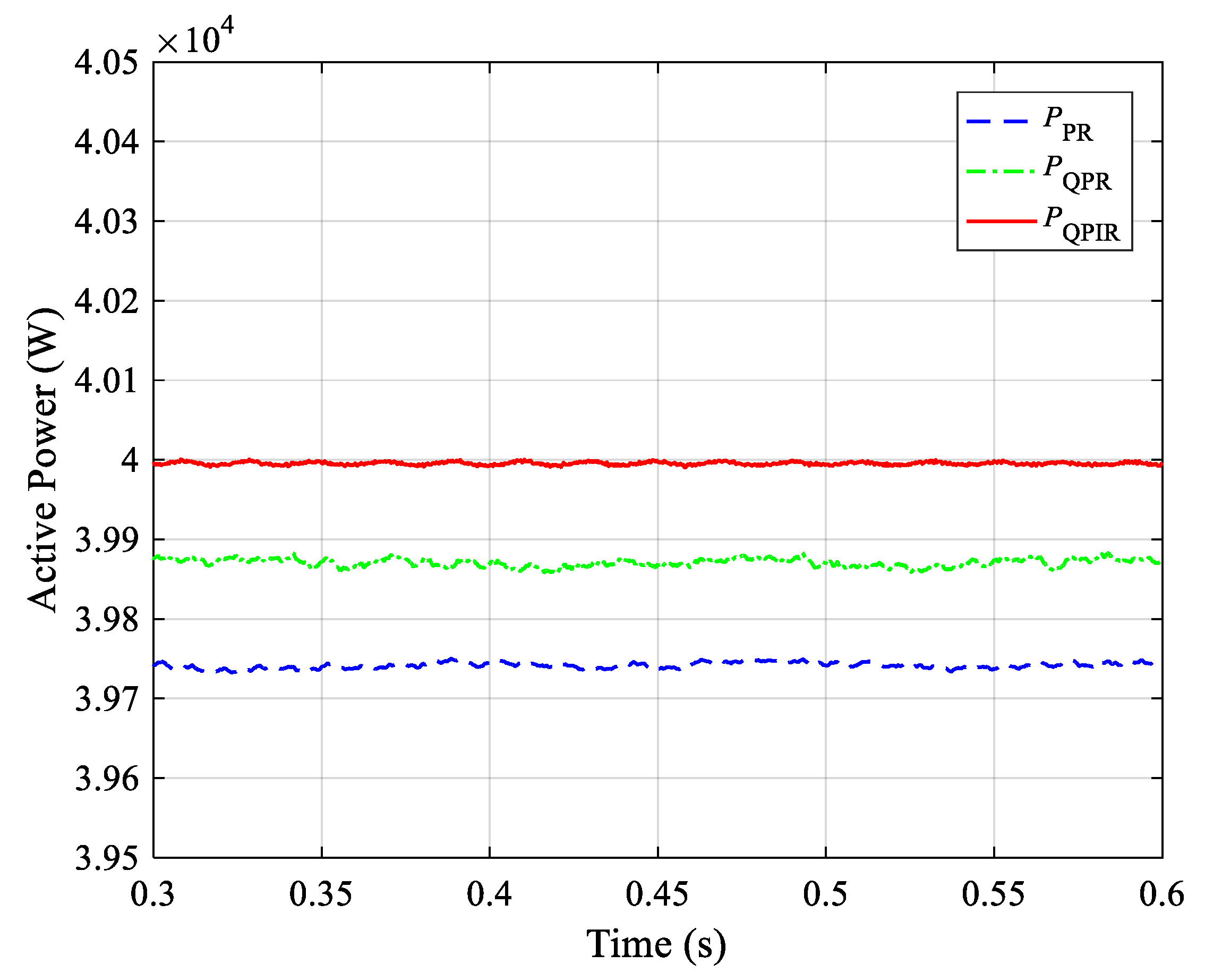
• Compared with the traditional PR and QPR controllers, the improved QPIR controller has higher grid-connected current control accuracy under the condition of stable and fluctuating grid frequency.
• The improved QPIR controller can realize the fast follow-up of active power and reactive power by the inverter, and when the active power jumps, the reactive power is not affected. When the reactive power jumps, the active power is not affected.

To sum up, the improved QPIR current controller proposed in this paper realizes the independent control of active power and reactive power of the three-phase grid-connected inverter in the two-phase static coordinate system. It also ensures the control accuracy and rapidity of the grid-connected current and has certain practical significance for high-power factor applications and improving the utilization rate of the DC side.

References

1. Hassaine, L.; OLias, E.; Quintero, J.; Salas, V. Overview of power inverter topologies and control structures for grid connected photovoltaic systems. Renew. Sustain. Energy Rev. 2014, 30, 796–807. [Google Scholar] [CrossRef]
2. Blaabjerg, F.; Teodorescu, R.; Liserre, M.; Timbus, A.V. Overview of Control and Grid Synchronization for Distributed Power Generation Systems. IEEE Trans. Ind. Electron. 2006, 53, 1398–1409. [Google Scholar] [CrossRef] [Green Version]
3. Gomes, C.C.; Cupertino, A.F.; Pereir, H.A. Damping techniques for grid-connected voltage source converters based on LCL filter: An overview. Renew. Sustain. Energy Rev. 2018, 81, 116–135. [Google Scholar] [CrossRef]
4. Nardi, C.; Stein, C.M.O.; Carati, E.G.; Costa, J.P.; Cardoso, R. A methodology of LCL filter design for grid-tied power converters. IEEE Trans. Ind. Electron. 2006, 53, 1398–1409. [Google Scholar]
5. Zhang, J.; Xiong, G.; Meng, K.; Yu, P.; Yao, G.; Dong, Z. An improved probabilistic load flow simulation method considering correlated stochastic variables. Int. J. Electr. Power Energy Syst. 2019, 111, 260–268. [Google Scholar] [CrossRef]
6. Zhang, J.; Fan, L.; Zhang, Y. A Probabilistic Assessment Method for Voltage Stability Considering Large Scale Correlated Stochastic Variables. IEEE Access 2020, 8, 5407–5415. [Google Scholar] [CrossRef]
7. Sahoo, A.K.; Shahani, A.; Basu, K.; Mohan, N. LCL filter design for grid-connected inverters by analytical estimation of PWM ripple voltage. In Proceedings of the IEEE Applied Power Electronics Conference and Exposition, Fort Worth, TX, USA, 16–20 March 2014; pp. 1281–1286. [Google Scholar]
8. Zhang, H.; Ruan, X.; Lin, Z.; Wu, L.; Ding, Y.; Guo, Y. Capacitor Voltage Full Feedback Scheme for LCL-Type Grid-Connected Inverter to Suppress Current Distortion Due to Grid Voltage Harmonics. IEEE Trans. Power Electron. 2021, 36, 2996–3006. [Google Scholar] [CrossRef]
9. Elsaharty, M.A.; Ashour, H.A. Passive L and LCL filter design method for grid-connected inverters. In Proceedings of the IEEE Conference in Innovative Smart Grid Technologies, Kuala Lumpur, Malaysia, 20–23 May 2014; pp. 13–18. [Google Scholar]
10. Li, N.; Wang, Y.; Niu, R.; Guo, W.; Lei, W.; Wang, Z. A novel LCL filter parameter design method basing on resonant frequency optimization method of three-level NPC grid connected inverter. In Proceedings of the IEEE Conference on Power Electronics, Hiroshima, Japan, 18–21 May 2014; pp. 160–165. [Google Scholar]
11. Reznik, A.; Simões, M.G.; Durra, A.A.; Muyeen, S.M. LCL filter design and performance analysis for grid interconnected systems. IEEE Trans. Ind. Appl. 2014, 50, 1225–1232. [Google Scholar] [CrossRef]
12. Alzola, R.P.; Liserre, M.; Blaabjerg, F.; Sebastián, R.; Dannehl, J.; Fuchs, F.W. Analysis of the passive damping losses in LCL-filter-based grid converters. IEEE Trans. Power Electron. 2013, 28, 2642–2646. [Google Scholar] [CrossRef] [Green Version]
13. Ahn, H.M.; Oh, C.Y.; Sung, W.Y.; Ahn, J.H.; Lee, B.K. Analysis and Design of LCL Filter with Passive Damping Circuits for Three-phase Grid-connected Inverters. In Proceedings of the IEEE 2015 9th International Conference on Power Electronics and ECCE Asia (ICPE-ECCE Asia), Seoul, Korea, 1–5 June 2015; pp. 1–5. [Google Scholar]
14. Pan, D.; Ruan, X.; Bao, C.; Li, W.; Wang, X. Capacitor-current feedback active damping with reduced computation delay for improving robustness of LCL-type grid-connected inverter. IEEE Trans. Power Electron. 2014, 29, 3414–3427. [Google Scholar] [CrossRef]
15. Jia, Y.; Zhao, J.; Fu, X. Direct Grid Current Control of LCL-Filtered Grid-Connected Inverter Mitigating Grid Voltage Disturbance. IEEE Trans. Power Electron. 2014, 29, 1532–1541. [Google Scholar]
16. Zou, Z.; Wang, Z.; Cheng, M. Modeling, Analysis, and Design of Multifunction Grid-Interfaced Inverters with Output LCL Filter. IEEE Trans. Power Electron. 2014, 29, 3830–3839. [Google Scholar] [CrossRef]
17. Dannehl, J.; Fuchs, F.W.; Hansen, S.; Paul, B.T. Investigation of active damping approaches for PI-based current control of gridconnected pulse width modulation converters with LCL filters. IEEE Trans. Ind. Appl. 2010, 46, 1509–1517. [Google Scholar] [CrossRef]
18. Xu, J.; Xie, S.; Tang, T. Active damping-based control for grid connected LCL-filtered inverter with injected grid current only. IEEE Trans. Ind. Electron. 2014, 61, 4746–4758. [Google Scholar] [CrossRef]
19. Hanif, M.; Khadkikar, V.; Xiao, W.; Kirtley, J.L. Two Degrees of Freedom Active Damping Technique for LCL Filter-Based Grid Connected PV Systems. IEEE Trans. Ind. Electron. 2014, 61, 2795–2830. [Google Scholar] [CrossRef]
20. Dannehl, J.; Fuchs, F.W.; Thøgersen, P.B. PI State Space Current Control of Grid-Connected PWM Converters With LCL Filters. IEEE Trans. Power Electron. 2010, 25, 2320–2330. [Google Scholar] [CrossRef]
21. Busada, C.A.; Jorge, S.G.; Solsona, J.A. Full-state feedback equivalent controller for active damping in LCL filtered grid connected inverters using a reduced number of sensors. IEEE Trans. Ind. Electron. 2015, 62, 5993–6002. [Google Scholar] [CrossRef]
22. Nishida, K.; Abded, T.; Nakaoka, M. A Novel Finite-Time Settling Control Algorithm Designed for Grid-Connected Three-Phase Inverter With an LCL-Type Filter. IEEE Trans. Ind. Appl. 2014, 50, 2005–2020. [Google Scholar] [CrossRef]
23. Yu, Y.; Li, H.; Li, Z.; Zhao, Z. Modeling and Analysis of Resonance in LCL-Type Grid-Connected Inverters under Different Control Schemes. Energies 2017, 10, 104. [Google Scholar] [CrossRef] [Green Version]
24. Dang, C.; Tong, X.; Song, W. Sliding-mode control in dq-frame for a three-phase grid-connected inverter with LCL-filter. ELSEVIER 2020, 357, 10159–10174. [Google Scholar] [CrossRef]
25. Zhang, H.; Xian, J.; Shi, J.; Wu, S.; Ma, Z. High Performance Decoupling Current Control by Linear Extended State Observer for Three-Phase Grid-Connected Inverter With an LCL Filter. IEEE Access 2020, 8, 13119–13127. [Google Scholar] [CrossRef]
26. Firuzi, M.F.; Roosta, A.; Gitizadeh, M. Stability analysis and decentralized control of inverter-based ac microgrid. Protection and Control of Modern Power Systems. 2019, 4, 65–86. [Google Scholar]
27. Badal, F.R.; Das, P.; Sarker, S.K.; Das, S.K. A survey on control issues in renewable energy integration and microgrid. Protection and Control of Modern Power Systems. 2019, 4, 87–113. [Google Scholar] [CrossRef] [Green Version]
28. Liserre, M.; Sauter, T.; Hung, J.Y. Future energy systems: Integrating renewable energy sources into the smart power grid through industrial electronics. IEEE Trans. Ind. Electron. 2010, 4, 18–37. [Google Scholar] [CrossRef]
29. Annamraju, A.; Nandiraju, S. Coordinated control of conventional power sources and PHEVs using jaya algorithm optimized PID controller for frequency control of a renewable penetrated power system. Prot. Control Mod. Power Syst. 2019, 4, 343–355. [Google Scholar] [CrossRef] [Green Version]
30. Tian, P.; Li, Z.; Hao, Z. Doubly-Fed Induction Generator Coordination Control Strategy Compatible with Feeder Automation. Electronics 2020, 9, 18. [Google Scholar] [CrossRef] [Green Version]
31. Komurcugil, H.; Altin, N.; Ozdemir, S.; Sefa, I. Lyapunov-function and proportional resonant based control strategy for single-phase grid-connected VSI with LCL filter. IEEE Trans. Ind. Electron. 2016, 63, 2838–2849. [Google Scholar] [CrossRef]
32. Alemi, P.; Jeong, S.; Jeong, S.Y.; Lee, D.C. Active Damping of LLCL Filters Using PR Control for Grid-Connected Three-Level T-Type Converters. Korean Institude Power Electron. 2015, 15, 786–795. [Google Scholar] [CrossRef]
33. Tian, P.; Li, Z.; Hao, Z. A Doubly-Fed Induction Generator Adaptive Control Strategy and Coordination Technology Compatible with Feeder Automation. Energies 2019, 12, 4463. [Google Scholar] [CrossRef] [Green Version]
34. Gong, Z.; Zheng, X.; Zhang, H.; Wu, X.; Li, M. A QPR-Based Low-Complexity Input Current Control Strategy for the Indirect Matrix Converters with Unity Grid Power Factor. IEEE Trans. Access. 2019, 99, 38766–38777. [Google Scholar] [CrossRef]
35. Tian, P.; Li, Z.; Hao, Z. Improved Controller of LCL-Type Grid-connected Inverter System based on Active-Damping. In Proceedings of the 2018 10th International Conference on Modelling, Identification and Control (ICMIC), Guiyang, China, 2–4 July 2018; pp. 1–6. [Google Scholar]
36. Craciun, B.I.; Kerekes, T.; Sera, D.; Teodorescu, R. Overview of recent grid codes for PV power integration. In Proceedings of the IEEE International Conference on Optimization of Electrical and Electronic Equipment, Brasov, Romania, 24–26 May 2012; pp. 959–965. [Google Scholar]
37. Bao, C.; Ruan, X.; Wang, X.; Li, W.; Pan, D.; Weng, K. Step-by-Step Controller Design for LCL-Type Grid-Connected Inverter with Capacitor Current-Feedback Active-Damping. IEEE Trans. Power Electron. 2014, 29, 1239–1253. [Google Scholar]
Figure 1. LCL-type three-phase grid-connected inverter topology.
Applsci 11 03170 g001
Figure 2. Threephase LCL-type grid-connected inverter with active damping in the α-β coordinate system.
Applsci 11 03170 g002
Figure 3. Control block diagram of the grid-connected inverter with LCL filter in the α-β coordinate system.
Applsci 11 03170 g003
Figure 4. Bode diagram of T(s) with capacitor current proportional feedback.
Applsci 11 03170 g004
Figure 5. Bode diagram of PR and QPR controllers.
Applsci 11 03170 g005
Figure 6. Bode diagram of PR, QPR, and QPIR controllers.
Applsci 11 03170 g006
Figure 7. Implementation block diagram of the QPIR controller.
Applsci 11 03170 g007
Figure 8. Bode diagram of T(s) with PR, QPR, and QPIR controllers.
Applsci 11 03170 g008
Figure 9. Steady-state waveforms of grid-connected current and voltage using PR, QPR, and QPIR controllers (at 49.5 Hz).
Applsci 11 03170 g009
Figure 10. Active power waveforms controlled by PR, QPR, and QPIR controllers (at 49.5 Hz).
Applsci 11 03170 g010
Figure 11. Reactive power waveforms controlled by PR, QPR, and QPIR controllers (at 49.5 Hz).
Applsci 11 03170 g011
Figure 12. Steady-state waveforms of grid-connected current and voltage using PR, QPR, and QPIR controllers (at 50.5 Hz).
Applsci 11 03170 g012
Figure 13. Active power waveforms controlled by PR, QPR, and QPIR controllers (at 50.5 Hz).
Applsci 11 03170 g013
Figure 14. Reactive power waveforms controlled by PR, QPR, and QPIR controllers (at 50.5 Hz).
Applsci 11 03170 g014
Figure 15. Step waveforms of active and reactive power.
Applsci 11 03170 g015
Figure 16. Step tracking waveforms of active and reactive power.
Applsci 11 03170 g016
Figure 17. Power grid frequency fluctuation diagram.
Applsci 11 03170 g017
Figure 18. Power waveforms controlled by the QPIR and PR controllers when the grid frequency fluctuates.
Applsci 11 03170 g018
Figure 19. Power waveforms controlled by the QPIR and QPR controllers when the grid frequency fluctuates.
Applsci 11 03170 g019