Efficient Attention Mechanism for Dynamic Convolution in Lightweight Neural Network

Abstract

Light-weight convolutional neural networks (CNNs) suffer limited feature representation capabilities due to low computational budgets, resulting in degradation in performance. To make CNNs more efficient, dynamic neural networks (DyNet) have been proposed to increase the complexity of the model by using the Squeeze-and-Excitation (SE) module to adaptively obtain the importance of each convolution kernel through the attention mechanism. However, the attention mechanism in the SE network (SENet) selects all channel information for calculations, which brings essential challenges: (a) interference caused by the internal redundant information; and (b) increasing number of network calculations. To address the above problems, this work proposes a dynamic convolutional network (termed as EAM-DyNet) to reduce the number of channels in feature maps by extracting only the useful spatial information. EAM-DyNet first uses the random channel reduction and channel grouping reduction methods to remove the redundancy in the information. As the downsampling of information can lead to the loss of useful information, it then applies an adaptive average pooling method to maintain the information integrity. Extensive experimental results on the baseline demonstrate that EAM-DyNet outperformed the existing approaches, thus it can achieve higher accuracy of the network test and less network parameters.

1. Introduction

In recent years, convolutional neural networks (CNNs) have been making great progress and success in image classification and description [1]. As the computation of CNNs involves a large number of parameters, they cannot be directly deployed on the emerging Internet of Things (IoT) end devices, which typically have limited resources [2] such as mobile phones, wireless sensor nodes, etc. Lightweight networks have gained great attention, since they require less computation than traditional CNNs (e.g., VggNet [3], ResNet [4], etc). Consequently, many lightweight networks have been conducted (e.g., MobileNet [5,6,7,8], ShuffleNet [9,10], etc). However, the number of parameters in lightweight networks is relatively small, which makes the fitting ability of data distribution insufficient. Dynamic neural networks (DyNet) [11,12,13] have been considered as a promising method to overcome this problem.

DyNet increases the network parameters so that it has powerful feature representation ability. Brandon Yang [11] added attention weights that are determined by the input of the convolution layer. Then, these weights are combined to obtain the convolution kernel weights. Yikang Zhang [12] obtained the attention weight by global average pooling and a fully connected layer. Yinpeng Chen [13] obtained the attention weight through a series of calculations such as compression, linear transformation, and weighing the sum with the convolution kernel. The models of these dynamic networks are shown in Figure 1. These dynamic networks use the Squeeze-and-Excitation (SE) attention module to weight multiple dynamic cores for dynamic perceptron cores. However, the dynamic convolutional networks have to compress all the feature maps to calculate the attention weights, which generates a lot of redundant information. A direct consequence is that it brings massive computation and potential interference. For the purpose of illustration, Figure 2 shows an example of visualizing the input image and the first layer of the dynamic convolution. It is obvious that the feature maps marked with the same color are very similar and have a great certain degree of redundancy. Therefore, it is crucial to extract the useful feature maps and remove the redundant ones, thereby achieving energy efficiency for the resource constrained IoT end devices.

In this work, it tries to extract representative feature information from all downsampled feature maps in every layer. For the extraction method of useful spatial information, it has been found that the feature similarity between neighbors is higher through visual feature maps. To obtain better features, we used random channel reduction (RCR) and channel group reduction (CGR) to extract spatial information to minimize redundancy. However, since we extracted the useful spatial information, if we continue to use the ordinary average pooling in dynamic convolution to downsample the useful information, some of them will be lost. Therefore, we tried to use adaptive pooling to downsample the useful information that had been extracted to output a tensor of a specified size to reduce the loss of useful information. The network is called Efficient Attention Mechanism for Dynamic Convolution Network (EAM-DyNet). The main contributions of this work can be summarized as follows:

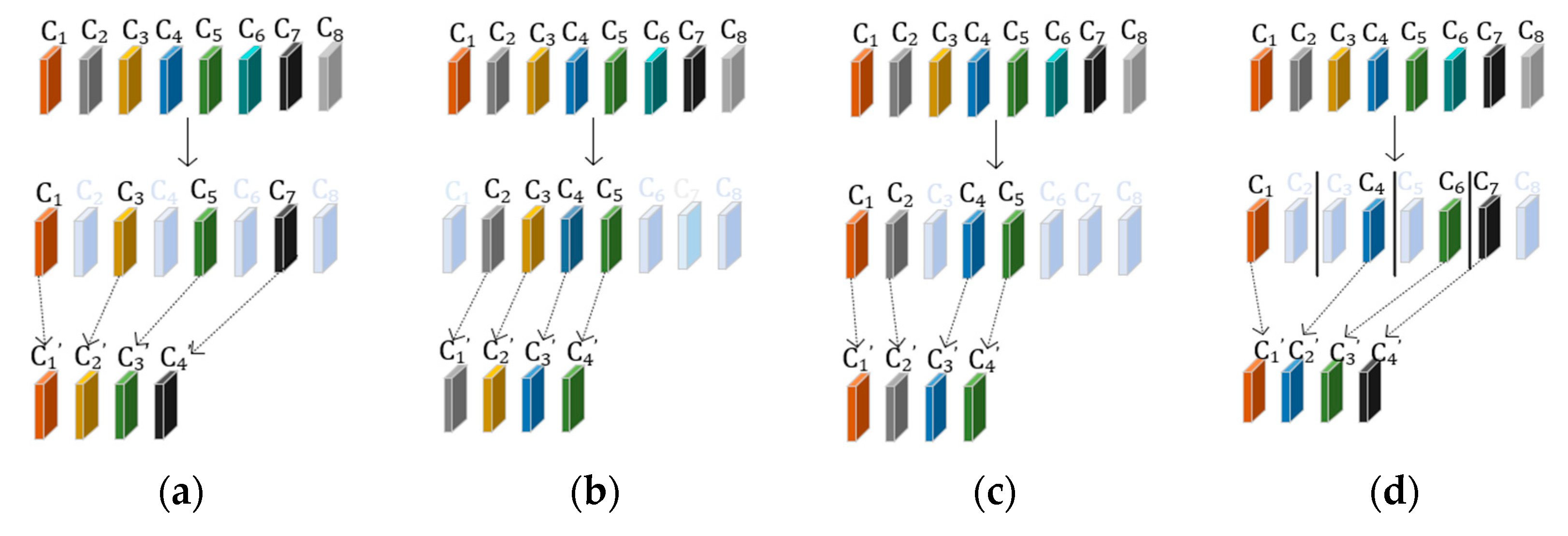
• It extracts useful spatial information in proportion to the interval of all feature maps to remove spatial features with similar features to reduce redundancy and the amount of calculation.
• It maintains the useful information when downsampling compared to the existing method of reducing spatial information to a one-dimensional vector.
• Through the verification of different types of networks of different widths, it was found that our method effectively reduced the value of floating-point operations per second (FLOPs) and improved the accuracy of the standard lightweight network and dynamic network.

The rest of this paper is organized as follows. Section 2 reviews the related works. Section 3 presents the proposed EAM-DyNet network. Section 4 evaluates its performance by extensive experimental results. Finally, Section 5 concludes this work.

2. Related Works

In this section, we introduce the related works of lightweight networks, DyNet, and the channel redundancy in CNNs.

2.1. Efficient Work

In recent years, lightweight networks [5,6,7,9,10,14,15] have been widely researched, reducing complexity and parameters. MobileNet [5,6,7], SqueezeNet [14], and ShuffleNet [9,10] are widely used. Among them, SqueezeNet [14] mainly describes that the 1 $\times$ 1 convolution kernel replaces the 3 $\times$ 3 convolution kernel as the compression module to splice with the original module to reduce the parameters. MobileNet V1 mainly uses depth-wise separable convolution [16] instead of traditional convolution, that is, a 3 $\times$ 3 convolution kernel is divided into depth-wise convolution and point-wise convolution [17], thereby reducing parameters and improving computing speed. Based on MobileNet V1, MobileNet V2 performs the linear transformation and adds a residual design by borrowing the idea of ResNet, however, unlike ResNet, MobileNet V2 replaces the standard convolution with depth-wise convolution to increase the number of channels inside the block. ShuffleNet reduces the amount of FLOPs and improves the calculation speed of the network by performing channel shuffle on the output of the group convolution. MnasNet [18] introduces the attention module of Squeeze-and-Excitation [8] to the residual network based on MobileNet V2. MobileNet V3 uses platform-aware neural architecture [19,20,21,22,23,24,25,26] to optimize each network block to search for the best network architecture. Later, Daniel et al. [27] proposed blueprint separable convolution, which is different from depth-wise separable convolution [16] in that pointwise convolution is performed first, and then depth-wise convolution. Compared with current networks, DyNet can achieve better results than static networks.

2.2. Dynamic Neural Networks (DyNet)

To increase the complexity of the model and improve the performance of neural networks, researchers have tried to make deep neural networks dynamic [28,29,30,31,32,33,34]. Among them, D2NN [29] combines backpropagation and reinforcement learning [35] to achieve dynamic effects. SkipNet [30] uses reinforcement learning methods to decide whether to implement a certain layer of the network to achieve dynamic goals. BlockDrop [31] uses the method of reinforcement learning to determine whether to use residual blocks. MSDnet [32] will determine whether the classifier outputs the result in advance, according to the confidence of the prediction. SlimmableNets [33] is to jointly train sub-networks of different widths in the same network model and share parameters. Once-For-All [34] uses the progressive shrinking approach to train the network to make the accuracy of the sub-network consistent with the effect of individual training. The above DyNet all have a static convolution kernel, but a dynamic network structure, while the recently proposed CondConv [11] and dynamic convolution [13] have a dynamic convolution kernel but a static network structure. CondConv [11] cleverly combines conditional calculation, integration technology, and attention mechanism, so that the network achieves high efficiency while having fewer parameters. Its method is similar to that in [8,36,37,38]. Dynamic convolution [13] adds dynamic attention weights in the convolution so that the static weight of the perceptron in the convolution is replaced by the dynamic weight affected by feature maps to achieve the effect of a dynamic network. However, these DyNet have a lot of redundancy while inputting feature maps, which increases the number of network parameters and affects the speed of network operations.

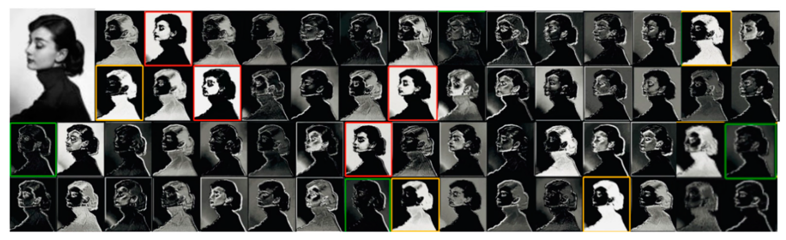
2.3. The Channel Redundancy in Convolutional Neural Networks (CNNs)

In DyNet, there is a lot of redundancy because feature maps are used as the input for calculating dynamic weights. In recent years, there are many models for solving redundancy. GhostNet [39] first generates inherent features from ordinary convolutions, and then obtains redundant feature maps through “cheap” linear operations to enhance features and achieve the effect of reducing redundancy. SPConv [40] divides all input channels into two parts; one part uses a $k\times k$ convolution kernel to extract the internal information from the representative part, and the other part uses point convolution to extract the detailed differences hidden in the uncertain redundant information. Through this operation, the features with similar patterns, but less calculation can be determined, thereby solving the problem of redundancy between feature maps. SPConv needs a relatively large amount of calculation while extracting internal information. Therefore, our model will compress the input feature information and extract the useful spatial information in the channel. Based on solving the redundancy problem, it also reduces the network calculation amount.

3. Proposed Efficient Attention Mechanism for Dynamic Convolution Network (EAM-DyNet)

This section first describes the standard model of dynamic networks, then proposes the network (denoted as EAM-DyNet) to address the issue of redundancy in the attention mechanism.

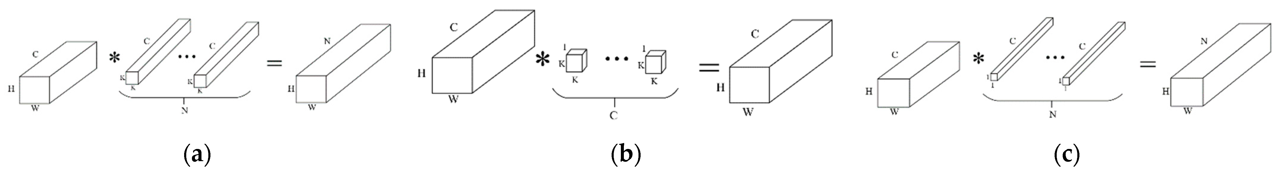
3.1. Lightweight Neural Networks

Lightweight neural networks use some convolution operations such as depth-wise separable convolution to make neural networks more lightweight. The depth-wise separable convolution is composed of a depth-wise convolution and a point-wise convolution, and the parameters of the convolution are smaller than that of standard convolution. Figure 3 shows these three convolution methods. Therefore, compared with the ordinary CNNs, it has a smaller number of parameters and less calculation.

In a lightweight neural network, it supposes an input image of size $C\times H\times W$ and defines the training set as

$$D_{label}^{image}=\left\{\left(x_t,y_t\right)\right\},$$

(1)

where $x_t$ is the $t$th input image and $y_t$ is the label corresponding to this image.

In the training process, it will estimate the parameter $\theta =\left\{W,b\right\}$, and its representation is:

$$\theta =\underset{\left\{W,b\right\}}{\arg \min }L\left(f\left(x_t\right),y_t\right),$$

(2)

$$f\left(x_t\right)=W\otimes x_t+b,$$

(3)

where $L(\cdot )$ is the loss function; $W$ is the weight during linear transformation; and $b$ is the corresponding bias.

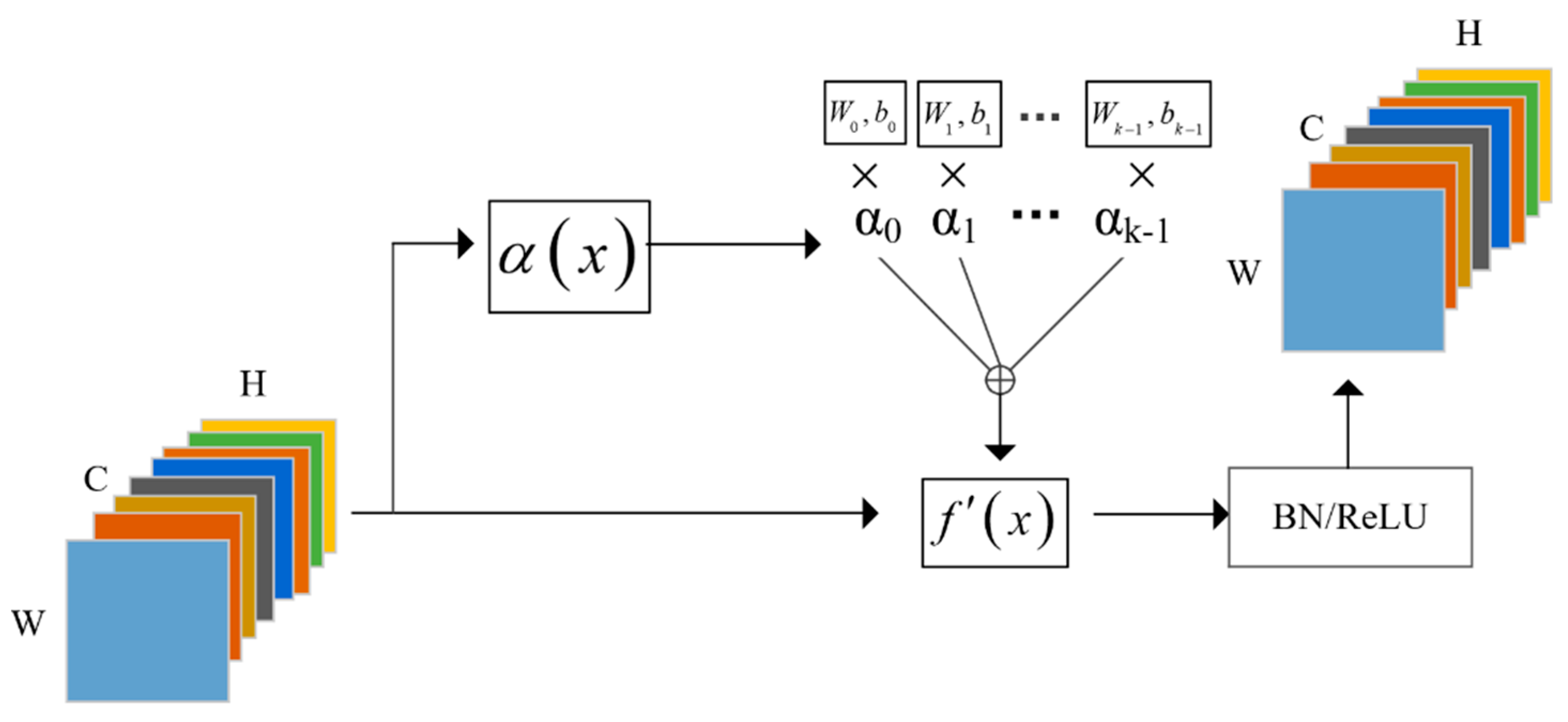
3.2. The Standard Model of Dynamic Network

To increase the complexity of the network, DyNet process the weight matrix. DyNet form a dynamic perceptron by adding an attention module to weight multiple dynamic cores. The static convolution weights will become dynamic weights by adding an attention mechanism, so that the neural network will also become a dynamic network. The calculations are as follows:

$$f^{\prime }\left(x\right)=W\left(x\right)\otimes x+b\left(x\right),$$

(4)

$$W\left(x\right)={\displaystyle \sum _{i=0}^{k-1}\left({\alpha }_i\left(x\right)\times \mathrm{k}\mathrm{e}\mathrm{r}\mathrm{n}\mathrm{e}{\mathrm{l}}_i\right)},$$

(5)

$$b\left(x\right)={\displaystyle \sum _{i=0}^{k-1}\left({\alpha }_i\left(x\right)\times b_i\right)},$$

(6)

$${\displaystyle \sum _{i=0}^{k-1}{\alpha }_i\left(x\right)}=1,$$

(7)

Among them, $\mathrm{k}\mathrm{e}\mathrm{r}\mathrm{n}\mathrm{e}{\mathrm{l}}_i$ is the input information in the $i$th convolution kernel; ${\alpha }_i\left(x\right)$ is used as the weight of attention to perform a weighted summation on the convolution kernel information, and its value is between 0 and 1. $W\left(x\right)$ is the dynamic weight matrix. After that, the dynamic weight matrix and the convolution kernel are convolved. Finally, it outputs the results after the activation function and optimized through batch processing. Figure 4 shows the model diagrams of standard dynamic convolution (DyNet) and channel reduction convolution (EAM-DyNet).

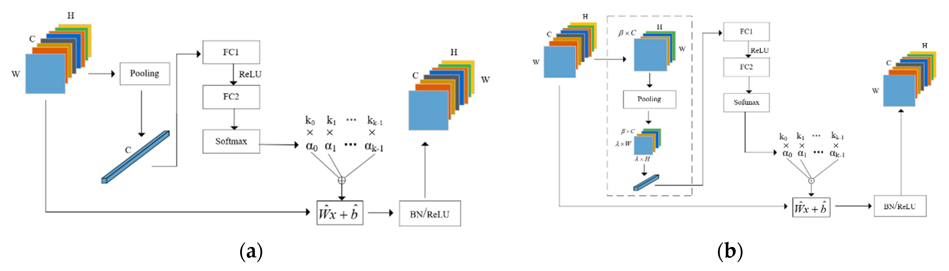
3.3. Efficient Attention Mechanism for Dynamic Convolution Network (EAM-DyNet)

While calculating the attention weights, the networks need to compress the information by the pooling layer and pass through two fully connected layers. A ReLU activation function is required in the middle of the fully connected layer. The size of the output from the fully connected layer should be consistent with the number of attention weights, that is, k, and finally, obtain the attention weight after softmax. In this process, we can select a part of the size of the information as the input of the attention weight to better reduce its redundancy because the input image will have a lot of redundant information. Therefore, we conducted the following processing for the spatial information of channel size $\stackrel{⌢}{C}$:

$$\stackrel{⌢}{C}=\beta C,$$

(8)

Among them, $\stackrel{⌢}{C}$ is the channel size of the selected channel information, where $\beta$ is a value from 0 to 1, and the size of the picture information should be $\beta \times C\times H\times W$. As it also verified different sizes of $\beta$ and selected different spatial information through different experiments, the accuracy rate will also change.

For the channel selection method, the main methods are channel adjacent reduction, channel equal interval reduction, random channel reduction (RCR) and channel group reduction (CGR).

The compression method is shown in Figure 5. If we assume the input channel $D=\left\{D_0,D_1,\cdots ,D_i,\cdots ,D_{C-1}\right\}$.

Channel Adjacent Reduction: This method selects continuous spatial information from the spatial information of channel size $C$. When selecting the channel of size $\stackrel{⌢}{C}$, we can select the first, middle, or last $\beta C$ channels, and select that these channels are adjacent and continuous. The formula can be expressed as:

$$\stackrel{⌢}{D}=\left\{D_j,D_{j+1},D_{j+2},\cdots ,D_{j+\stackrel{⌢}{C}}\right\},$$

(9)

$$0\le j\le C-\stackrel{⌢}{C}-1,$$

(10)

Channel Equal Interval Reduction: To avoid the possibility of redundant information generated between adjacent channels, it selects spatial information at equal intervals. When selecting $\stackrel{⌢}{C}$ channels from the spatial information of channel size $C$, we will take one time every $1/\beta$ channels, then $\beta \times C$ channels are taken out, that is, $\stackrel{⌢}{C}$ channels. Its expression is shown in Equation (11).

$$\stackrel{⌢}{D}=\left\{D_0,D_{\frac{1}{\beta }},D_{\frac{2}{\beta }},\cdots ,D_{\frac{\beta \times C-1}{\beta }}\right\},$$

(11)

Random Channel Reduction (RCR): To reduce redundancy to a greater extent, it randomly takes out $\stackrel{⌢}{C}$ from the spatial information of channel size $C$ in this method. When the value of $\stackrel{⌢}{C}$ is equal to the number of attention cores $k$, the effect is best by a series of experiments. Its expression is shown in Equation (12).

$$\stackrel{⌢}{D}=\left\{{\stackrel{⌢}{D}}_0,{\stackrel{⌢}{D}}_1,\cdots ,{\stackrel{⌢}{D}}_{\stackrel{⌢}{C}}\right\},$$

(12)

$$\stackrel{⌢}{D}\subseteq D,$$

(13)

Channel Group Reduction (CGR): In the RCR-based method, we can optimize it by grouping these channels to avoid the uncertainty of using the RCR method. To obtain the best spatial information of the $k$ channels, it equally divides the $C$ channels into $k$ blocks, selects one channel from each block, and selects $k$ channels in total. When randomly selecting from each block, it is called group random compression (CGR-Random). When the maximum spatial information is selected from each block, it is called CGR-MAX. Its expression is shown in Equation (14).

$$\stackrel{⌢}{D}=\left\{{\stackrel{⌢}{D}}_0,{\stackrel{⌢}{D}}_1,\cdots ,{\stackrel{⌢}{D}}_j,\cdots ,{\stackrel{⌢}{D}}_k\right\},$$

(14)

$${\stackrel{⌢}{D}}_j\subseteq \left\{D_{\frac{j\times C}{k}},\cdots ,D_{\frac{\left(j+1\right)\times C}{k}}\right\},$$

(15)

In the process of addressing the attention weight, DyNet use pooling to compress the images, but the ordinary pooling layer compresses an $H\times W$ size image into a $1\times 1$ size image, which leads to the loss of spatial information due to the reduction in channels. Therefore, to address this problem, EAM-DyNet uses adaptive pooling to compress the channel information to output the channel information of the specified size. Finally, after pooling, the size of the spatial information will be reduced by ${\beta }^2$ times, that is, the size of the spatial information should be ${\beta }^2\times H\times W$ at this time. In the adaptive pooling layer, the output tensor size is determined by the input size, kernel size, and stride. The calculation of the output size is as follows:

$$outpu{t}_{size}=\frac{(inpu{t}_{size}+2\times \mathrm{p}\mathrm{a}\mathrm{d}\mathrm{d}\mathrm{i}\mathrm{n}\mathrm{g}-\mathrm{k}\mathrm{e}\mathrm{r}\mathrm{n}\mathrm{e}{\mathrm{l}}_{size})}{stride}+1,$$

(16)

Therefore, to obtain the output size we need, the adaptive pooling layer will automatically adjust its $\mathrm{k}\mathrm{e}\mathrm{r}\mathrm{n}\mathrm{e}{\mathrm{l}}_{size}$ and $stride$ to achieve an adaptive effect.

However, the choice of different pooling also has a certain impact on the experimental results. Commonly used adaptive pooling layers include the adaptive average pooling layer and adaptive maximum pooling layer. The average pooling layer divides the input information into several groups, compresses these groups of data by averaging them, and finally outputs the required results, while the maximum pooling layer compresses each group of data by taking the maximum value. We can find which pooling layer is more effective by comparing the accuracy of two pooling layers experimentally.

After this, we input the feature map with the size of ${\beta }^2\times C\times H\times W$ into the fully connected layer. After passing through the first fully connected layer, we reduced the channel size to 10, then the channel size was reduced to k by the second fully connected layer, which is the number of attention cores. In addition, there is the ReLU activation function between two fully connected layers. Finally, it uses softmax to obtain the attention weights. However, when the softmax is set to 1 and multiple kernels cannot be optimized at the same time, this will lead to slow training convergence speed and affect the experimental results. Therefore, to address this low-efficiency problem, we set it to a larger temperature, and the calculation method is as shown in the formula:

$${\alpha }_i=\frac{\exp (\frac{c_i}{\tau })}{{\displaystyle \sum _j\exp (\frac{c_j}{\tau })}},$$

(17)

Among them, $c_i$ is the output result of the $i$th attention weight from the second fully connected layer, and τ is the temperature. By setting the size of different temperatures, we finally found that the training result would be more effective when τ is 30, and the final accuracy rate will reach the highest.

4. Experimental Results

This section describes the experimental setup and numerous results.

4.1. Experimental Setup

This work mainly verified the performance of our model on image classification. All experiments used the well-known Pytorch deep learning architecture. The experiment was carried out on an UltraLAB graphics workstation. The workstation is equipped with 192 G memory, 8 NVIDIA RTX-2080 graphics processors, and each graphics card had 8 G existing memory. The image workstation used the Windows server operating system. We used three standard benchmark datasets, namely CIFAR10, CIFAR100, and ImageNet100.

4.1.1. CIFAR10 and CIFAR100

The CIFAR 10/100 datasets [41] contained 10 and 100 categories and have 50,000 training images and 10,000 test images, with a size of 32 px $\times$ 32 px. Through [4,42], we know that two datasets are to be trained for 200 epochs. We used SGD to optimize, and its momentum and weight decay were respectively set to 0.9 an ${10}^{-4}$. Furthermore, we used an adjustable learning rate, which was initially set to 0.1 and dropped by 0.1 times at the 100th, 150th, and 180th epochs. To prevent overfitting [4,42], our image was increased by up to 4 px during random horizontal flip and shift. For the input image during training, we padded 4 pixels on each side of the image, and a 32 × 32 crop was randomly sampled from the padded image or its horizontal flip. Through the above, data augmentation operates to prevent overfitting during training.

4.1.2. ImageNet100

In the image classification experiment, the public dataset we used was the ILSVRC2012 dataset [43] including training images, evaluation images, and test images. Each group had 1000 classes, of which 1,281,167 images were used for training, 50,000 images were used for validation, and 50,000 images were used for the test. We took every 10 classes from 1000 classes, took out 100 classes, and randomly selected 500 images from each class in the train-set, and randomly took 50 images from the corresponding class in the test-set to form ImageNet100.

Furthermore, we also used ratio enhancement [44], horizontal flip, and color dithering [1] to adjust the image, which made the size 256 px. At this time, our batch size was set to 128.

Training setup for MobilenetV1: We used an initial learning rate of 0.1 to train for 120 epochs and attenuate it by a factor of 0.2 at the 30th, 60th, and 90th epochs. The models used SGD with a momentum of 0.9 and a weight decay of ${10}^{-4}$ for optimization.

Training setup for MobilenetV2 and MobilenetV3: The initial learning rate was 0.05, and was scheduled to reach zero within a single cosine period for 300 epochs. The models used SGD with a momentum of 0.9 and a weight decay of ${10}^{-4}$ for optimization.

4.1.3. Baseline

This article mainly conducted verification on a lightweight network. The network mainly selected MobilenetV1 $\times$ 1.0, MobilenetV2 $\times$ 1.0, MobilenetV3_small $\times$ 1.0, and MobilenetV3_large $\times$ 1.0 for verification and selected different widths from MobilenetV1 $\times$ 0.25, MobilenetV1 $\times$ 0.5, MobilenetV1 $\times$ 0.75, and MobilenetV1 $\times$ 1.0 for verification on dynamic networks with different widths. In addition, two GPUs were used when training the MobilenetV2 $\times$ 1.0 and MobilenetV3_large $\times$ 1.0, and the rest of the models used a single-core GPU.

4.1.4. Model

Suppose we input a picture of size $C\times H\times W$; $C$ is the channel size; and $H\times W$ is the channel information size. In this article, the number of attention cores $k$ was 4, and we used RCR and CGR to extract useful spatial information. Since the number of cores $k$ was 4, we extracted the useful information of the four channels. Then, the adaptive average pool will compress the spatial information of these four channels with the $5\times 5$ size of the compressed output. The output passes through two fully connected layers (there is a ReLU activation function between the two layers), where the output of the first fully connected layer is 10, and the output of the second fully connected layer is the number of attention cores $k$. Then, the input to the softmax function with temperature, where the temperature τ was set to 30, the four attention weights were output as ${\alpha }_i\left(x\right)$, and then after the ${\displaystyle \sum _{i=0}^{k-1}\left({\alpha }_i\left(x\right)\times \mathrm{k}\mathrm{e}\mathrm{r}\mathrm{n}\mathrm{e}{\mathrm{l}}_i\right)}$ weighting operation to obtain the required weight of the perceptron during convolution. After that, the output of the perceptron is processed by the Batch-normal and ReLU activation function to obtain our improved convolution output.

Since the mid-channel in MobilenetV2 is very large, when using the CGR method to reduce the channel, if a channel is randomly selected from each group, some useful information will be lost and the experimental results will be affected. Therefore, the channel with the largest tensor is extracted from each group, so that the extracted information is more useful and the accuracy rate is higher. We marked this method as CGR-MAX in the table.

4.2. Numerous Results

4.2.1. Baseline Results

For an input picture of size $C_{in}\times H\times W$, if we assume that the output of convolution is $C_{out}$ and the kernel size is $D_H\times D_W$, then it has $C_{in}\times D_H\times D_W\times C_{out}+C_{out}$ parameters. In the dynamic convolution kernel, it is composed of dynamic attention and dynamic convolution. If the input and output of the first fully connected layer are $\stackrel{⌢}{C}$ and $C_{out1}$, the output of the second fully connected layer is $k$, and the output of pooling is ${\lambda }^2\times H\times W$. Therefore, the attention needs $\stackrel{⌢}{C}\times C_{out1}+C_{out1}\times k+C_{out1}+k$ parameters and the parameters of dynamic convolution are $k\times C_{in}\times D_H\times D_W\times C_{out}+k\times C_{out}$. Similarly, for the FLOPs of the network, the FLOPs required by each attention is $O\left(\alpha \left(x\right)\right)={\lambda }^2\times H\times W\times \stackrel{⌢}{C}+2\times \stackrel{⌢}{C}\times C_{out1}+2\times C_{out1}\times k$ and the FLOPs of dynamic convolution is $O\left(f^{\prime }\left(x\right)\right)=\left(2\times k\times C_{in}\times D_H\times D_W+k-1\right)\times H\times W$. For DyNet, when solving attention parameters and FLOPs, $\stackrel{⌢}{C}=C_{in}$. As the network depth increases, the value of $\stackrel{⌢}{C}$ is larger. However, for EAM-DyNet, the size of $\stackrel{⌢}{C}$ is always equal to k. As the network gets deeper, the value of $\stackrel{⌢}{C}$ of DyNet is much larger than k, so the parameters and FLOPs are also higher than EAM-DyNet. For example, EAM-DyNet’s parameters and FLOPs were reduced by 1.38 M and 6.15 M, respectively, relative to DyNet on MobilenetV1. On MobilenetV2, the parameters and FLOPs of EAM-DyNet were reduced by 2.27 M and 8.92 M relative to DyNet. However, the accuracy of EAM-DyNet was increased by 0.43% and 0.56% compared to DyNet on two baselines.

The results of the top-1 accuracy on the baseline are shown in

Table 1. The accuracy of different architectures on CIFAR10, CIFAR100, and ImageNet100.

Network	CIFAR10	CIFAR100	ImageNet100
	Top-1 (%)	Top-1 (%)	Top-1 (%)
MobilenetV1 × 1.0	93.83	74.41	75.27
DyNet MobilenetV1 × 1.0	93.99	74.76	75.94
EAM-DyNet MobilenetV1 × 1.0 + RCR	93.61	74.83	76.37
EAM-DyNet MobilenetV1 × 1.0 + CGR	93.93	75.21	76.11
DyNet MobilenetV1 × 0.75	93.50	73.54	74.14
EAM-DyNet MobilenetV1 × 0.75 + RCR	93.49	73.88	74.67
EAM-DyNet MobilenetV1 × 0.75 + CGR	93.55	74.04	74.51
DyNet MobilenetV1 × 0.5	93.15	72.31	72.27
EAM-DyNet MobilenetV1 × 0.5 + RCR	92.70	72.85	72.93
EAM-DyNet MobilenetV1 × 0.5 + CGR	92.78	72.42	72.15
DyNet MobilenetV1 × 0.25	91.14	68.30	66.76
EAM-DyNet MobilenetV1 × 0.25 + RCR	91.01	68.61	68.50
EAM-DyNet MobilenetV1 × 0.25 + CGR	91.12	68.71	67.25
MobilenetV2 × 1.0	93.60	74.90	77.66
DyNet MobilenetV2 × 1.0	94.09	75.50	78.11
EAM-DyNet MobilenetV2 × 1.0 + RCR	94.07	75.23	78.67
EAM-DyNet MobilenetV2 × 1.0 + CGR-MAX	94.22	75.44	78.26
DyNet MobilenetV3_small × 1.0	91.97	73.10	69.22
EAM-DyNet MobileneV3_small × 1.0 + RCR	91.93	72.14	69.65
EAM-DyNet MobileneV3_ small × 1.0 + CGR-MAX	92.13	72.42	70.64
MobilenetV3_large × 1.0	93.70	75.20	76.36
DyNet MobilenetV3_large × 1.0	94.15	75.03	76.37
EAM-DyNet MobileneV3_large × 1.0 + RCR	94.00	74.77	76.62
EAM-DyNet MobileneV3_large × 1.0 + CGR-MAX	94.20	75.15	76.37

DyNet is a standard dynamic network, and EAM-DyNet was our model. After the ‘+’ is the method used to select the channel. After the ‘×’ is the width of the network.

, in addition to comparing the parameters and FLOPs of DyNet MobilenetV1 $\times$ 1.0, EAM-DyNet MobilenetV1 $\times$ 1.0, DyNet MobilenetV2 $\times$ 1.0, and EAM-DyNet MobilenetV2 $\times$ 1.0. The comparison results are shown in

Table 2. The parameter value and FLOPs value of MobilenetV1 and MobilenetV2 in ImageNet100.

Network	ImageNet100 Top-1 (%)	Parameters	FLOPs
DyNet MobilenetV1 × 1.0	75.94	14.27M	589.70M
EAM-DyNet MobilenetV1 × 1.0 + RCR	76.37 (+0.43)	12.89M (−9.6%)	583.55M
EAM-DyNet MobilenetV1 × 1.0 + CGR	76.11	12.89M (−9.6%)	583.55M
DyNet MobilenetV2 × 1.0	78.11	11.25M	336.34M
EAM-DyNet MobilenetV2 × 1.0 + RCR	78.67 (+0.56)	8.98M (−20.17%)	327.42M
EAM-DyNet MobilenetV2 × 1.0 + CGR	78.26	8.98M (−20.17%)	327.42M

. From the experimental results, it was found that the EAM-DyNet reduced the number of network parameters and the FLOPs value compared to the DyNet. In addition, the accuracy of EAM-DyNet was lower than that of DyNet. Among them, the CGR method was better on the CIFAR dataset, and the RCR method on the ImageNet100 dataset was better. For MobilenetV1 × 1.0, the accuracy of the CIFAR dataset can be increased by 0.45% and the accuracy of the Imagenet dataset could be the largest increase by 0.43%. For MobilenetV2 $\times$ 1.0, it greatly reduced the number of network parameters and increased the characterization ability of the network.

4.2.2. Ablation Studies Results

A series of ablation experiments were conducted on MobilenetV1 $\times$ 1.0. In these experiments, we set the default number of attention cores $k$ to 4, and the temperature τ of softmax to 30.

The number of channels: The choice of channel size and number of channels determine the degree to which the model reduces its redundancy. It defaults the pooling layer to adaptive average pooling, and the output size of the pooling is $5\times 5$ spatial information.

When EAM-DyNet uses the RCR method with different sizes of channel on different datasets, namely two channels, four channels, and eight channels. The experimental results are shown in

Table 3. The accuracy of standard static network, standard dynamic network, and EAM-DyNet when using the Random Channel Reduction (RCR) method to take out channels of different sizes on MobilenetV1.

The Number of Channels (RCR)	CIFAR10	CIFAR100	ImageNet100
	Top-1 (%)	Top-1 (%)	Top-1 (%)
DyNet MobilenetV1 × 1.0	93.99	74.76	75.94
EAM-DyNet MobilenetV1 × 1.0 (2 channels)	93.95	74.50	75.78
EAM-DyNet MobilenetV1 × 1.0 (4 channels)	93.61	74.83	76.37
EAM-DyNet MobilenetV1 × 1.0 (8 channels)	94.07	74.70	75.45

. After experimental verification, it was found that when the selected channel was the same size as the attention core, and its accuracy rate reached the highest. Compared with the standard static and standard dynamic networks, the EAM-DyNet network increased by 1.1 and 0.43 percentage points.

The methods of channel reduction: For the selection method of different channels, EAM-DyNet uses $1/4C$ as the default size, and chooses $0~1/4C$, $1/4C~1/2C$, $1/2C~3/4C$, $3/4C\text{~}C$, then takes every four channels to compare their results with the RCR and CGR methods, and the results are shown in

Table 4. The accuracy of standard static network, standard dynamic network, and EAM-DyNet in different channel selection methods on MobilenetV1.

The Methods of Channels Selection	CIFAR10	CIFAR100	ImageNet100
	Top-1 (%)	Top-1 (%)	Top-1 (%)
DyNet MobilenetV1 × 1.0	93.99	74.76	75.94
EAM-DyNet MobilenetV1 (take every 4 channels)	93.72	74.84	76.58
EAM-DyNet MobilenetV1 × 1.0 (0~1/4C)	93.79	74.38	75.92
EAM-DyNet MobilenetV1 × 1.0 (1/4C~1/2C)	93.90	75.18	75.20
EAM-DyNet MobilenetV1 × 1.0 (1/2C~3/4C)	93.62	75.03	75.80
EAM-DyNet MobilenetV1 × 1.0 (3/4C~C)	94.03	74.99	76.23
EAM-DyNet MobilenetV1 × 1.0(RCR)	93.61	74.83	76.37
EAM-DyNet MobilenetV1 × 1.0(CGR)	93.93	75.21	76.11

. In addition, it calculates the parameters and FLOPs when choosing the channel of $1/4C$ size and choosing the channel with the RCR and CGR method, the result of calculation is shown in

Table 5. The parameters and FLOPs of different channel selection methods on EAM-DyNet MobilenetV1.

Network	ImageNet100 Top-1 (%)	Parameters	FLOPs
EAM-DyNet MobilenetV1 × 1.0 (1/4C)	76.58	13.48M	585.17M
EAM-DyNet MobilenetV1 × 1.0 + RCR	76.37	8.98M	583.55M
EAM-DyNet MobilenetV1 × 1.0 + CGR	76.11	8.98M	583.55M

. After comparing the FLOPs, the parameters, and the accuracy rate of different methods, we found that when using the RCR and CGR methods, the parameter amount and FLOPs were the lowest, but the accuracy rate was high. The reason why the calculation amount is too high when $1/4C$ is selected is because as the network becomes deeper, the number of channels will increase, and the calculation amount will increase. However, the channels selected by RCR and CGR were always four channels. Through the results in the two tables, we found that the parameters and FLOPs of the RCR and CGR methods were reduced by 4.5 M and 257.75 M, but the accuracy remained flat or even greater than the other method.

The selection of pooling and its output size: Pooling is used to compress spatial information. The pooling selection method and output size determine the degree of retention of spatial information. In the experiment, our default channel size was 4, and the channel method was RCR. For the choice of adaptive pooling, experiments were conducted on adaptive average pooling and adaptive maximum pooling. The output size was set to $5\times 5$ by default. The experimental results are shown in

Table 6. The accuracy rate when using different pooling on EAM-DyNet MobilenetV1.

The Selection of Pooling	CIFAR10	CIFAR100	ImageNet100
	Top-1 (%)	Top-1 (%)	Top-1 (%)
DyNet MobilenetV1 × 1.0	93.99	74.76	75.94
EAM-DyNet MobilenetV1 × 1.0 (AdaptAvgPool)	93.61	74.83	76.37
EAM-DyNet MobilenetV1 × 1.0 (AdaptMaxPool)	93.89	74.91	76.50

. Experiments show that the effects of the two poolings were not too different. Therefore, it used adaptive average pooling by default.

We made an additional experiment without retaining spatial information. This experiment was to train in the ImageNet100 dataset. The baseline was MobilenetV1. It directly downsampled the reduced channel to one dimension. We found that it caused the loss of useful information. The experiment found that its accuracy was 76.02%. Therefore, to preserve the spatial information of some selected channels when downsampling, we chose adaptive pooling. To verify that adaptive pooling could retain spatial information, we selected the output spatial information of different sizes for comparison. The selected sizes were $3\times 3$, $5\times 5$, and $7\times 7$. The comparison results are shown in

Table 7. The accuracy of adaptive pooling with different output sizes on EAM-DyNet MobilenetV1.

The Output Size of AdaptAvgPool	CIFAR10	CIFAR100	ImageNet100
	Top-1 (%)	Top-1 (%)	Top-1 (%)
DyNet MobilenetV1 × 1.0	93.99	74.76	75.94
EAM-DyNet MobilenetV1 × 1.0 (3 × 3)	94.08	74.56	75.84
EAM-DyNet MobilenetV1 × 1.0 (5 × 5)	93.61	74.83	76.37
EAM-DyNet MobilenetV1 × 1.0 (7 × 7)	93.73	74.27	76.27

. Through the results, it was found that when it preserved the spatial information on some selected channels, the accuracy was higher than when downsampling the reduced channel to one dimension. In addition, when $5\times 5$ was selected, the effect was better.

5. Conclusions

In this work, we found that there is redundant information in the dynamic convolutional network with an attention mechanism. To solve this problem, we proposed an effective dynamic convolutional network, EAM-DyNet, which can reduce the redundancy of spatial information by reducing the number of channels in the feature map and extract useful spatial information. Then, due to the loss of useful information when downsampling the information, it uses an adaptive average pooling method to maintain the information integrity. The effectiveness of our model was verified through experiments on different datasets and different baseline networks. The results showed that EAM-DyNet not only increased the accuracy, but also reduced the number of network parameters and FLOPs compared to the existing approaches.

References

1. Krizhevsky, A.; Sutskever, I.; Hinton, G.E. ImageNet Classification with Deep Convolutional Neural Networks. Commun. ACM 2017, 60, 84–90. [Google Scholar] [CrossRef]
2. Huang, Y.; Yu, W.; Ding, E.; Garcia-Ortiz, A. EPKF: Energy efficient communication schemes based on Kalman filter for IoT. IEEE Internet Things J. 2019, 6, 6201–6211. [Google Scholar] [CrossRef]
3. Simonyan, K.; Zisserman, A. Very deep convolutional networks for large-scale image recognition. arXiv 2014, arXiv:1409.1556. [Google Scholar]
4. He, K.; Zhang, X.; Ren, S.; Sun, J. Deep residual learning for image recognition. In Proceedings of the 2016 IEEE Conference on Computer Vision and Pattern Recognition (CVPR), Las Vegas, NV, USA, 27–30 June 2016; pp. 770–778. [Google Scholar]
5. Howard, A.; Sandler, M.; Chu, G.; Chen, L.-C.; Chen, B.; Tan, M.; Wang, W.; Zhu, Y.; Pang, R.; Vasudevan, V.; et al. Searching for MobileNetV3. In Proceedings of the 2019 IEEE/CVF International Conference on Computer Vision, Seoul, Korea, 27 October–4 November 2019; pp. 1314–1324. [Google Scholar]
6. Howard, A.G.; Zhu, M.; Chen, B.; Kalenichenko, D.; Wang, W.; Weyand, T.; Andreetto, M.; Adam, H. MobileNets: Efficient convolutional neural networks for mobile vision applications. arXiv 2017, arXiv:1704.04861. [Google Scholar]
7. Sandler, M.; Howard, A.; Zhu, M.L.; Zhmoginov, A.; Chen, L.C. MobileNetV2: Inverted residuals and linear bottlenecks. In Proceedings of the 2018 IEEE/CVF International Conference on Computer Vision, Munich, Germany, 8–14 September 2018; pp. 4510–4520. [Google Scholar]
8. Hu, J.; Shen, L.; Albanie, S.; Sun, G.; Wu, E. Squeeze-and-excitation networks. IEEE Trans. Pattern Anal. Mach. Intell. 2020, 42, 2011–2023. [Google Scholar] [CrossRef] [PubMed] [Green Version]
9. Ma, N.; Zhang, X.; Zheng, H.-T.; Sun, J. ShuffleNet V2: Practical guidelines for efficient CNN architecture design. In Proceedings of the European Conference on Computer Vision (ECCV), Munich, Germany, 8–14 September 2018; pp. 122–138. [Google Scholar]
10. Zhang, X.; Zhou, X.; Lin, M.; Sun, J. ShuffleNet: An extremely efficient convolutional neural network for mobile devices. In Proceedings of the 2018 IEEE/CVF Conference on Computer Vision and Pattern Recognition, Munich, Germany, 8–14 September 2018; pp. 6848–6856. [Google Scholar]
11. Yang, B.; Bender, G.; Le, Q.V.; Ngiam, J. CondConv: Conditionally parameterized convolutions for efficient inference. In Advances in Neural Information Processing Systems 32, Proceedings of the Annual Conference on Neural Information Processing Systems 2019, NeurIPS 2019, Vancouver, BC, Canada, 8–14 December 2019; Wallach, H., Larochelle, H., Beygelzimer, A., d’Alche-Buc, F., Fox, E., Garnett, R., Eds.; NeurIPS: San Diego, CA, USA, 2019; Volume 32. [Google Scholar]
12. Zhang, Y.; Zhang, J.; Wang, Q.; Zhong, Z. DyNet: Dynamic convolution for accelerating convolutional neural networks. arXiv 2020, arXiv:2004.10694. [Google Scholar]
13. Chen, Y.; Dai, X.; Liu, M.; Chen, D.; Yuan, L.; Liu, Z. Dynamic convolution: Attention over convolution kernels. arXiv 2019, arXiv:1912.03458. [Google Scholar]
14. Iandola, F.N.; Han, S.; Moskewicz, M.W.; Ashraf, K.; Dally, W.J.; Keutzer, K. SqueezeNet: AlexNet-level accuracy with 50× fewer parameters and <0.5 MB model size. arXiv 2016, arXiv:1602.07360. [Google Scholar]
15. Wu, B.; Wan, A.; Yue, X.; Jin, P.; Zhao, S.; Golmant, N.; Gholaminejad, A.; Gonzalez, J.; Keutzer, K. Shift: A zero FLOP, zero parameter alternative to spatial convolutions. arXiv 2017, arXiv:1711.08141. [Google Scholar]
16. Sifre, L.; Mallat, S. Rigid-motion scattering for texture classification. arXiv 2014, arXiv:1403.1687. [Google Scholar]
17. Chollet, F. Xception: Deep learning with depthwise separable convolutions. In Proceedings of the 2017 IEEE Conference on Computer Vision and Pattern Recognition (CVPR), Honolulu, HI, USA, 21–26 July 2017; pp. 1800–1807. [Google Scholar]
18. Tan, M.; Chen, B.; Pang, R.; Vasudevan, V.; Sandler, M.; Howard, A.; Le, Q.V. MnasNet: Platform-aware neural architecture search for mobile. In Proceedings of the 2019 IEEE Conference on Computer Vision and Pattern Recognition (CVPR), Long Beach, CA, USA, 15–20 June 2019; pp. 2815–2823. [Google Scholar]
19. Zoph, B.; Le, Q.V. Neural architecture search with reinforcement learning. arXiv 2016, arXiv:1611.01578. [Google Scholar]
20. Yang, T.-J.; Howard, A.; Chen, B.; Zhang, X.; Go, A.; Sandler, M.; Sze, V.; Adam, H. NetAdapt: Platform-aware neural network adaptation for mobile applications. In Proceedings of the 2018 IEEE/CVF International Conference on Computer Vision, Munich, Germany, 8–14 September 2018; pp. 289–304. [Google Scholar]
21. Cai, H.; Zhu, L.; Han, S. ProxylessNAS: Direct neural architecture search on target task and hardware. arXiv 2018, arXiv:1812.00332. [Google Scholar]
22. Guo, Z.; Zhang, X.; Mu, H.; Heng, W.; Liu, Z.; Wei, Y.; Sun, J. Single path one-shot neural architecture search with uniform sampling. arXiv 2019, arXiv:1904.00420. [Google Scholar]
23. Zoph, B.; Vasudevan, V.; Shlens, J.; Le, Q.V. Learning transferable architectures for scalable image recognition. In Proceedings of the 2018 IEEE/CVF International Conference on Computer Vision, Salt Lake City, UT, USA, 18–23 June 2018; pp. 8697–8710. [Google Scholar]
24. Real, E.; Aggarwal, A.; Huang, Y.P.; Le, Q.V. Regularized evolution for image classifier architecture search. In Proceedings of the Thirty-Third AAAI Conference on Artificial Intelligence (AAAI-2019), Honolulu, HI, USA, 27 January 27–1 February 2019; pp. 4780–4789. [Google Scholar]
25. Liu, H.; Simonyan, K.; Yang, Y. DARTS: Differentiable architecture search. arXiv 2018, arXiv:1806.09055. [Google Scholar]
26. Xie, S.; Zheng, H.; Liu, C.; Lin, L. SNAS: Stochastic neural architecture search. arXiv 2018, arXiv:1812.09926. [Google Scholar]
27. Haase, D.; Amthor, M. Rethinking depthwise separable convolutions: How intra-kernel correlations lead to improved MobileNets. In Proceedings of the 2020 IEEE/CVF Conference on Computer Vision and Pattern Recognition (CVPR), Seattle, WA, USA, 13–19 June 2020; pp. 14588–14597. [Google Scholar]
28. Lin, J.; Rao, Y.; Lu, J.; Zhou, J. Runtime neural pruning. In Advances in Neural Information Processing Systems 30, Proceedings of the Annual Conference on Neural Information Processing Systems 2017, NeurIPS 2017, Long Beach, CA, USA, 4–9 December 2017; Guyon, I., Luxburg, U.V., Bengio, S., Wallach, H., Fergus, R., Vishwanathan, S., Garnett, R., Eds.; NeurIPS: San Diego, CA, USA, 2017; Volume 30. [Google Scholar]
29. Liu, L.; Deng, J. Dynamic deep neural networks: Optimizing accuracy-efficiency trade-offs by selective execution. In Proceedings of the Thirty-Second AAAI Conference on Artificial Intelligence (AAAI-18), New Orleans, LA, USA, 2–7 February 2018. [Google Scholar]
30. Wang, X.; Yu, F.; Dou, Z.-Y.; Darrell, T.; Gonzalez, J.E. SkipNet: Learning dynamic routing in convolutional networks. In Proceedings of the 2018 IEEE/CVF International Conference on Computer Vision, Munich, Germany, 8–14 September 2018; pp. 420–436. [Google Scholar]
31. Wu, Z.; Nagarajan, T.; Kumar, A.; Rennie, S.; Davis, L.S.; Grauman, K.; Feris, R. BlockDrop: Dynamic inference paths in residual networks. In Proceedings of the 2018 IEEE/CVF International Conference on Computer Vision, Salt Lake City, UT, USA, 18–23 June 2018; pp. 8817–8826. [Google Scholar]
32. Huang, G.; Chen, D.; Li, T.; Wu, F.; van der Maaten, L.; Weinberger, K.Q. Multi-scale dense networks for resource efficient image classification. arXiv 2017, arXiv:1703.09844. [Google Scholar]
33. Yu, J.; Huang, T. Universally slimmable networks and improved training techniques. In Proceedings of the 2019 IEEE/CVF International Conference on Computer Vision, Seoul, Korea, 27 October–4 November 2019; pp. 1803–1811. [Google Scholar]
34. Cai, H.; Gan, C.; Wang, T.; Zhang, Z.; Han, S. Once-for-all: Train one network and specialize it for efficient deployment. arXiv 2019, arXiv:1908.09791. [Google Scholar]
35. Mnih, V.; Kavukcuoglu, K.; Silver, D.; Graves, A.; Antonoglou, I.; Wierstra, D.; Riedmiller, M. Playing Atari with deep reinforcement learning. arXiv 2013, arXiv:1312.5602. [Google Scholar]
36. Luong, M.-T.; Pham, H.; Manning, C.D. Effective approaches to attention-based neural machine translation. arXiv 2015, arXiv:1508.04025. [Google Scholar]
37. Bahdanau, D.; Cho, K.; Bengio, Y. Neural machine translation by jointly learning to align and translate. arXiv 2014, arXiv:1409.0473. [Google Scholar]
38. Vaswani, A.; Shazeer, N.; Parmar, N.; Uszkoreit, J.; Jones, L.; Gomez, A.N.; Kaiser, Ł.; Polosukhin, I. Attention is all you need. In Proceedings of the 31st International Conference on Neural Information Processing Systems, Long Beach, CA, USA, 4–9 December 2017; pp. 6000–6010. [Google Scholar]
39. Han, K.; Wang, Y.; Tian, Q.; Guo, J.; Xu, C.; Xu, C. GhostNet: More features from cheap operations. In Proceedings of the 2020 IEEE/CVF Conference on Computer Vision and Pattern Recognition (CVPR), Seattle, WA, USA, 13–19 June 2020; pp. 1577–1586. [Google Scholar]
40. Zhang, Q.; Jiang, Z.; Lu, Q.; Han, J.n.; Zeng, Z.; Gao, S.-h.; Men, A. Split to be slim: An overlooked redundancy in vanilla convolution. arXiv 2020, arXiv:2006.12085. [Google Scholar]
41. Krizhevsky, A. Learning Multiple Layers of Features from Tiny Images. Master’s Thesis, University of Toronto, Toronto, ON, Canada, 2012. [Google Scholar]
42. Zagoruyko, S.; Komodakis, N. Wide residual networks. arXiv 2016, arXiv:1605.07146. [Google Scholar]
43. Russakovsky, O.; Deng, J.; Su, H.; Krause, J.; Satheesh, S.; Ma, S.; Huang, Z.; Karpathy, A.; Khosla, A.; Bernstein, M.; et al. ImageNet large scale visual recognition challenge. Int. J. Comput. Vis. 2015, 115, 211–252. [Google Scholar] [CrossRef] [Green Version]
44. Szegedy, C.; Wei, L.; Yangqing, J.; Sermanet, P.; Reed, S.; Anguelov, D.; Erhan, D.; Vanhoucke, V.; Rabinovich, A. Going deeper with convolutions. In Proceedings of the 2015 IEEE Conference on Computer Vision and Pattern Recognition (CVPR), Boston, MA, USA, 7–12 June 2015; pp. 1–9. [Google Scholar]
Figure 1. Model of dynamic convolutional network. In the figure, C is the channel size of feature maps; H and W are the size of spatial information; α ( x ) is the Squeeze-and-Excitation (SE) attention module; f ( x ) is the dynamic perceptron core; and W i , b i is the dynamic core.
Applsci 11 03111 g001
Figure 2. Visualize the input images of the dynamic MobileNet V1 and the feature maps of the first layer. Select similar feature maps from them and mark them with red, yellow, and green boxes. The feature maps marked with the same color are basically the same, so select representative feature maps can be used for input, and the remaining redundant information will increase the number of network parameters.
Applsci 11 03111 g002
Figure 3. (a) Standard convolution filters, (b) depth-wise convolution filters, (c) point-wise convolution filters. In the figure, K × K is the kernel size; C is the number of input channels; H × W is the size of spatial information; and N is the number of output channels; * is a convolution operation.
Applsci 11 03111 g003
Figure 4. (a) Model diagram of the dynamic neural networks (DyNet) in which the size of the output from the pooling layer is C × 1 × 1 , (b) model diagram of EAM-DyNet. Our method first selects representative spatial information, then uses adaptive pooling to compress the spatial information, k i is kernel i in Equation (5).
Applsci 11 03111 g004
Figure 5. In the figure, C i channel is the input channel, C i is the selected channel, and the main selection methods are as follows: (a) Channel adjacent reduction: C channels are selected from adjacent channels; (b) Channel equal interval reduction: 1 / β channels are selected at every interval, and β C channels are selected, namely C channels; (c) Random channel reduction (RCR): take out k channels randomly from C input channels; (d) Channel group reduction (CGR): divide C input channels into k blocks and take out one channel from each block, when k channels are taken out at random, it is recorded as CGR-Random; when taken out, the k largest channels from each block are denoted as CGR-MAX.
Applsci 11 03111 g005