
Influence of Maxwell Stiffness in Damage Control and Analysis of Structures with Added Viscous Dampers


Abstract
Featured Application
Abstract
1. Introduction
2. Materials and Methods
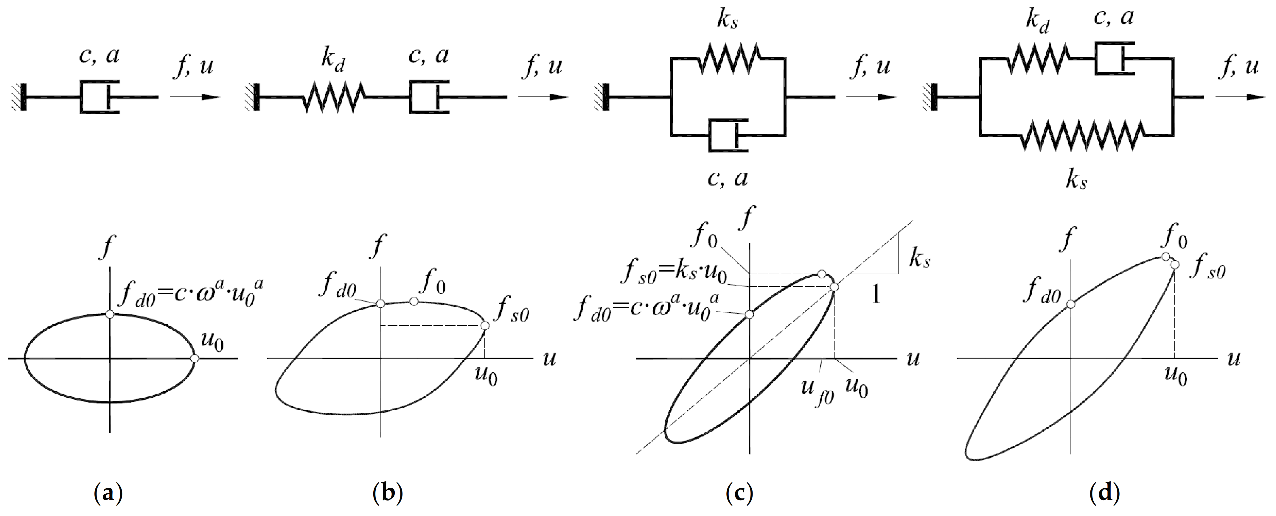
2.1. Mathematical Models
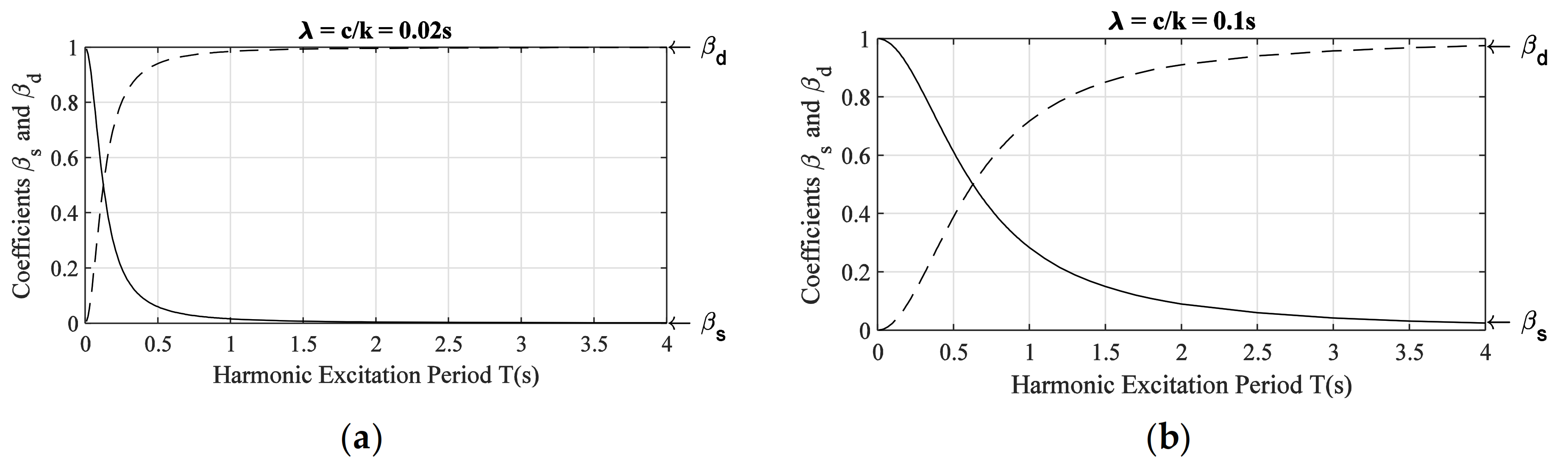
2.2. Estimate of Maxwell Stiffness
2.3. Numerical Study
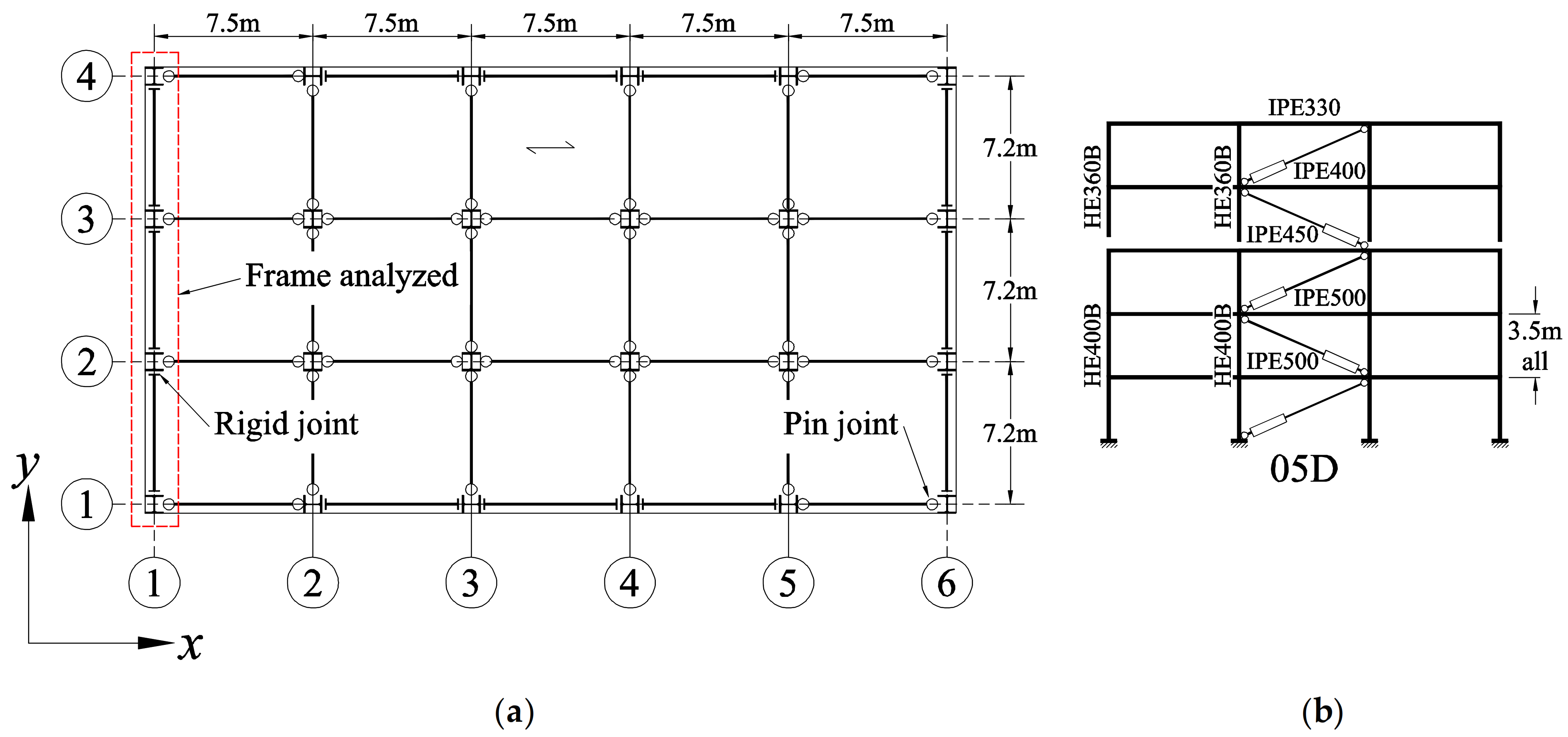
2.3.1. Description of Moment Resisting Frames (MRFs)
2.3.2. Description of Ground Motion Sets (GMS)
2.3.3. Seismic Intensities
2.3.4. Description of Added Damping Systems (ADS)
- The first letter (“Q” in the example) indicates the height-wise distribution (Q, R, S); the “Q” distribution has constant damping coefficients at all storeys; in the “R” and “S” distribution the damping coefficients decrease linearly with height up to a fraction of the first storey damping coefficient, 2/3 for the “R” distribution and 1/3 for the “S” distribution. Only complete vertical distributions are considered.
- The second number (“2” in the example) indicates the relative amount of damping in the first mode; for linear dampers, “1” indicates 11%, “2” indicates 23% and “3” indicates 34%; for non-linear dampers, the values are drift-dependent, but the damping coefficients keep a similar progression.
- The third number (“1” in the example) indicates the damper exponent: “1” indicates linear (a = 1) and “5” indicates non-linear (a = 0.5). All dampers in one ADS are either linear or non-linear.
2.3.5. Description of Analysis Models
2.3.6. Description of Brace Stiffness Model Options
- RB, modeled with a very large stiffness (1000 kN/mm).
- HB, in which the stiffness is calculated using the brace extender cross section and total diagonal centerline length.
- MB, in which the stiffness is taken as 50% that of the HB model.
- LB, in which the stiffness is taken as 25% that of the HB model.
2.3.7. Variables Analyzed
3. Results
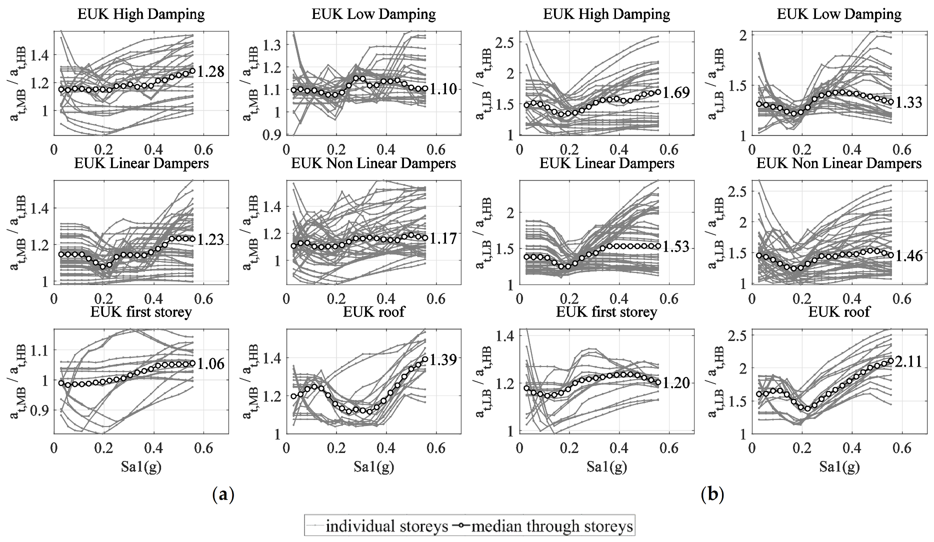
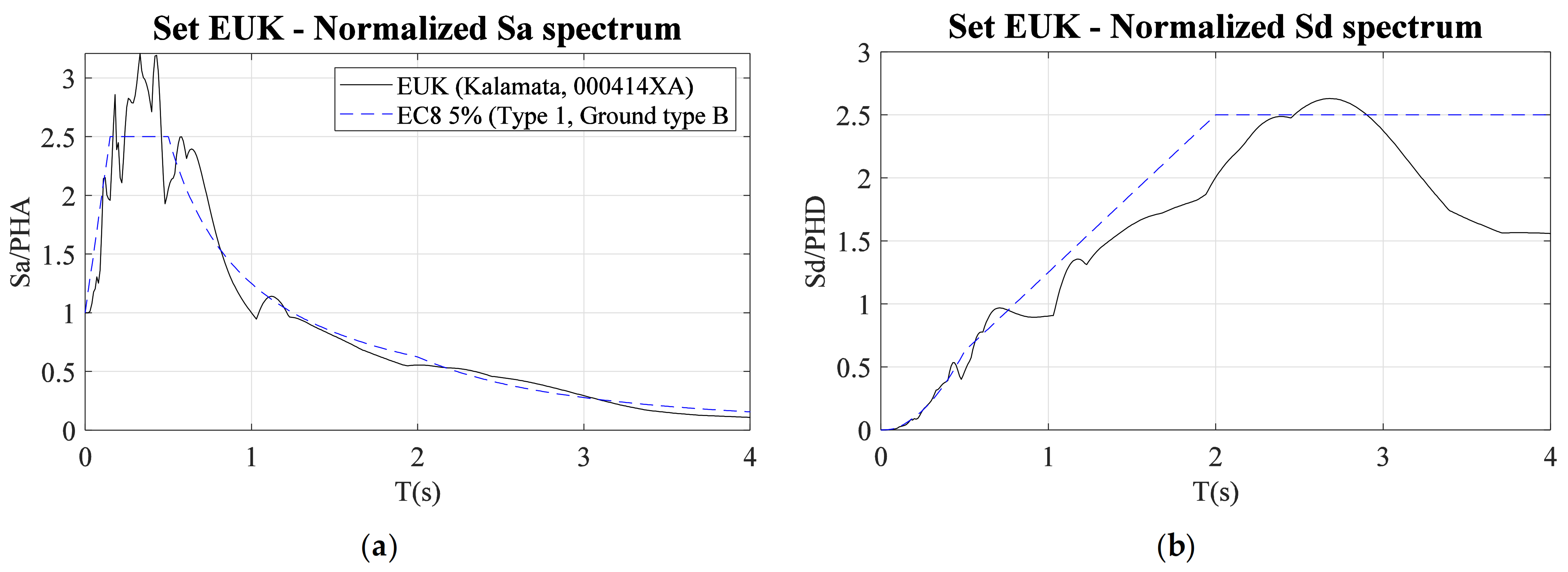
3.1. Results for One Motion (GMS EUK)
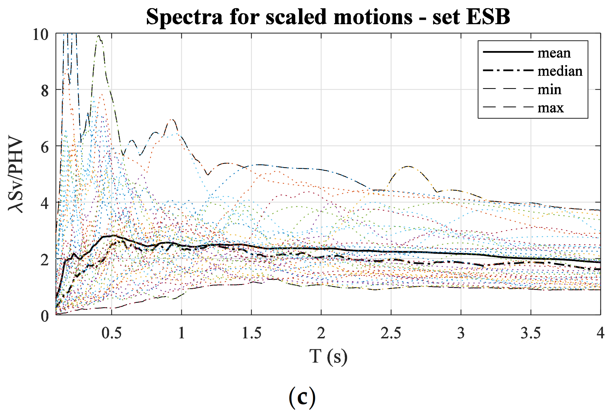
3.2. Results for Set of Motions (GMS ESB)
4. Discussion
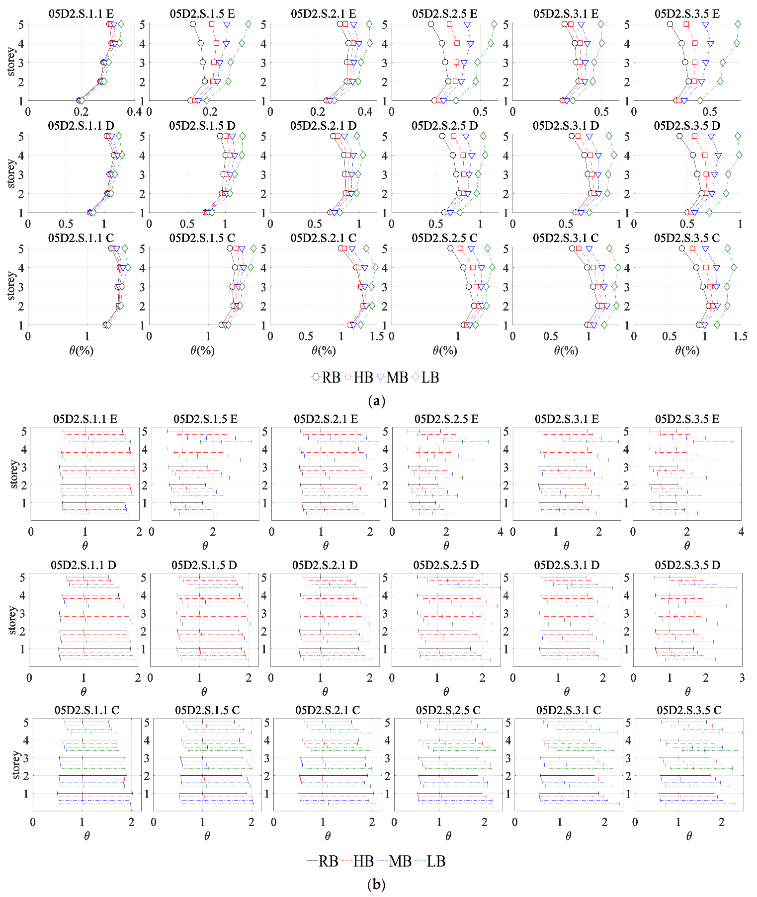
4.1. Drift
- Larger for non-linear dampers (1.34) than for linear dampers (1.17).
- Larger for increasing damping (1.11 for low damping to 1.37 for high damping).
- Almost unaffected by the type of damper distribution (1.27, 1.25, 1.24 for distributions Q, R, S).
- Much larger for the top half of the building (1.15 for first storey, 1.53 for roof).
4.2. Residual Drift
- Uninfluenced by the damper type; the ratio is very similar for linear dampers (2.07) and non-linear dampers (1.94).
- Larger for increasing damping (1.38 for low damping to 2.50 for high damping).
- Moderately influenced by the type of damper distribution (1.74; 1.88; 2.40 for distributions Q, R, S).
- Much larger for the top half of the building (1.56 for first storey, 2.79 for roof).
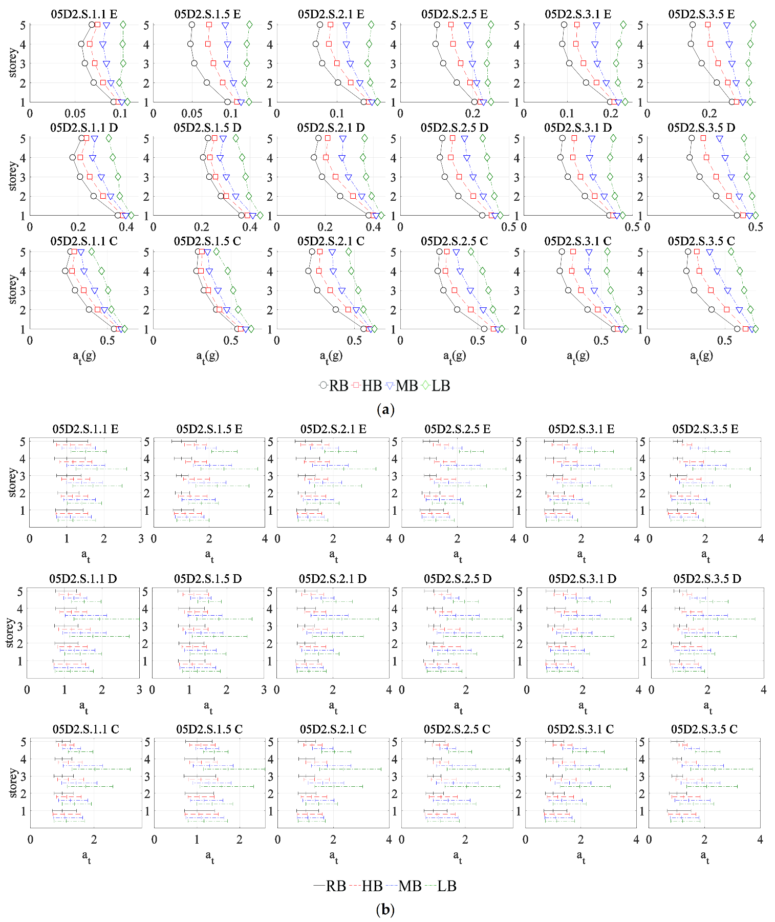
4.3. Total Acceleration
- Uninfluenced by the damper type (1.47 for linear dampers, 1.47 for non-linear dampers).
- Moderately influenced by the amount of damping (1,36 for low damping, 1.50 for high damping).
- Almost uninfluenced by the damper distribution (1.50 for Q, 1.44 for S).
- Larger for the roof (1.65) than for the first storey (1.15).
- Almost uninfluenced by the level of intensity (1.48 for level E vs. 1.47 for level C).
4.4. Relative Energy Input
4.5. Energy Dissipated by Damping System and Damper Shear
4.6. Plastic Strain Energy Dissipated by Frame, Columns and Beams
- Largely influenced by the type of damper (8.32 for linear dampers versus 15.95 for non-linear dampers).
- Largely influenced by the amount of damping (2.7 for low damping to 23.69 for high damping).
- Largely influenced by the damper distribution (7.33 for type Q, 19.43 for type S).
- Larger for the roof (25.30) than for the first storey (1.67).
4.7. Storey Shear and Total Shear
- Larger for non-linear dampers (1.50) than for linear dampers (1.31).
- Larger for increasing damping (1.19 for low damping to 1.57 for high damping).
- Almost unaffected by the type of damper distribution (1.46, 1.41, 1.34 for distributions Q, R, S).
- Much larger for the top half of the building (1.12 for first storey, 2.03 for roof).
- Larger for moderate intensity (1.52 for intensity level E, 1.33 for intensity level C).
4.8. Member Internal Forces
- Larger for non-linear dampers (1.32) than for linear dampers (1.16).
- Larger for increasing damping (1.36 for low damping to 1.09 for high damping).
- Almost unaffected by the type of damper distribution (1.28, 1.24, 1.20 for distributions Q, R, S).
- Much larger for the top half of the building (1.09 for first storey, 1.58 for roof).
- Larger for moderate intensity (1.38 for intensity level E, 1.13 for intensity level C).
- Larger for non-linear dampers (1.44) than for linear dampers (1.25).
- Larger for increasing damping (1.16 for low damping to 1.49 for high damping).
- Almost unaffected by the type of damper distribution (1.37, 1.34, 1.32 for distributions Q, R, S).
- Much larger for the top half of the building (1.09 for first storey, 1.81 for roof).
- Larger for moderate intensity (1.47 for intensity level E, 1.25 for intensity level C).
4.9. Member Rotation
4.10. Summary
- Quite large for the top part of the frame and moderate or negligible at the bottom part of the frame.
- Larger for models type LB (25% Maxwell stiffness) than for models type MB (50% Maxwell stiffness).
- Larger for moderate seismic intensities than for high seismic intensities.
- Larger for high damping than for low damping.
- Larger for non-linear dampers than for linear dampers.
- Variables with small sensitivity to Maxwell stiffness: relative energy input, damper shear, column axial force.
- Variables with large sensitivity to Maxwell stiffness: residual drift, absolute acceleration, plastic strain energy dissipated by frame, columns and beams.
- For non-linear dampers and/or high damping, the sensitivity of storey shear, column moment, beam and column rotation is large.
- For the top part of the frame, the sensitivity of all variables except energy input, column axial force and damper shear is large.
- Likewise, for the bottom part of the frame the sensitivity for all variables except residual drift, plastic strain energy and column rotation is small.
4.11. Minimum Maxwell Stiffness
5. Conclusions
- Relative energy input, damper shear and column axial force show a small sensitivity to the reduction in damping system stiffness.
- Residual drift, absolute acceleration and plastic strain energy dissipated by frame elements show a large sensitivity to the reduction in damping system stiffness.
- For non-linear dampers and/or high damping ratios: storey shear, column moment, beam rotation and column rotation show a large sensitivity to reduction in damping system stiffness.
- All other variables show a moderate sensitivity to reduction in damping system stiffness.
- 5.
- At the bottom part of the frame, only residual drift, plastic strain energy and column rotation are highly sensitive to reduction in damping system stiffness.
- 6.
- At the top part of the frame all variables are highly sensitive to variation in damping system stiffness, except energy input, column axial force and damper shear.
- Analysis was carried out for only two damper exponents (a = 1, a = 0.5). Comparison between trends for linear and non-linear cases in the study suggests an equal or larger sensitivity to Maxwell stiffness for lower damper exponents (a < 0.5). Additional work is needed to validate this assumption.
- The influence of horizontal distribution of dampers among bays has not been explored.
- Only simple vertical distributions of damping coefficients have been considered.
Supplementary Materials
Author Contributions
Funding
Institutional Review Board Statement
Informed Consent Statement
Data Availability Statement
Conflicts of Interest
Appendix A. Ground Motion Selection Information


| Name | Station | Date | Fault | Mw | Epic. Dist. (km) | PHAX (g) | PHAY (g) | Prescaleλx (1) | Prescaleλy (1) |
|---|---|---|---|---|---|---|---|---|---|
| Friuli (aftershock) | Forgaria-Cornio | 15.09.1976 | thrust | 6 | 17 | 0.264 | 0.218 | 2.861 | 2.085 |
| Friuli (aftershock) | Forgaria-Cornio | 15.09.1976 | thrust | 6 | 17 | 0.346 | 0.336 | 2.230 | 1.537 |
| Montenegro | Bar-SkupstinaOpstine | 15.04.1979 | thrust | 6.9 | 16 | 0.375 | 0.363 | 0.909 | 0.720 |
| Montenegro (aftershock) | Tivat-Aerodrom | 24.05.1979 | thrust | 6.2 | 21 | 0.166 | 0.133 | 2.481 | 2.198 |
| Montenegro (aftershock) | Petrovac-Hotel Oliva | 15.05.1979 | oblique | 5.8 | 24 | 0.099 | 0.089 | 1.451 | 1.211 |
| Campano Lucano | Calitri | 23.11.1980 | normal | 6.9 | 16 | 0.156 | 0.176 | 0.707 | 0.768 |
| Kalamata | Kalamata-Prefecture | 13.09.1986 | normal | 5.9 | 10 | 0.215 | 0.297 | 0.819 | 0.982 |
| Kyllini | Zakynthos-OTE Building | 16.10.1988 | strike slip | 5.9 | 14 | 0.151 | 0.146 | 0.685 | 1.367 |
| Erzincan | Erzincan-Meteorologij | 13.03.1992 | strike slip | 6.6 | 13 | 0.389 | 0.513 | 0.765 | 1.164 |
| Tithorea | Aigio-OTE Building | 18.11.1992 | normal | 5.9 | 25 | 0.038 | 0.028 | 0.807 | 1.932 |
| Umbria Marche | Gubbio-Piana | 26.09.1997 | normal | 6 | 38 | 0.091 | 0.097 | 0.838 | 0.760 |
| Potenza | Brienza | 05.05.1990 | strike slip | 5.8 | 28 | 0.096 | 0.080 | 2.208 | 1.534 |
| AnoLlosia | Athens 2 (Chalandri District) | 07.09.1999 | normal | 6 | 20 | 0.110 | 0.161 | 2.121 | 2.411 |
| Griva | Edessa-Prefecture | 21.12.1990 | normal | 6.1 | 36 | 0.101 | 0.096 | 0.899 | 1.100 |
| South Aegean | Heraklio-Technical University | 23.05.1994 | oblique | 6.1 | 45 | 0.061 | 0.041 | 1.212 | 0.814 |
| Strofades | Zakynthos-OTE Building | 18.11.1997 | oblique | 6.6 | 38 | 0.131 | 0.116 | 1.152 | 1.542 |
| Kozani | Kastoria-OTE Building | 13.05.1995 | normal | 6.5 | 50 | 0.019 | 0.020 | 1.024 | 1.272 |
| Aigion | Patra-San Dimitrios Church | 15.06.1995 | normal | 6.5 | 43 | 0.084 | 0.093 | 0.713 | 0.976 |
| Duzce 1 | LDEO Station No C1058 BV | 12.11.1999 | oblique | 7.2 | 11 | 0.111 | 0.073 | 1.257 | 1.044 |
| Firuzabad | Firoozabad | 20.06.1994 | strike slip | 5.9 | 22 | 0.250 | 0.278 | 3.366 | 3.481 |
| Vs30 | PHA | PHV | PHD | Epicentral Distance | Mw | Arias Intensity Ia | Significant Duration D5–95% | |
|---|---|---|---|---|---|---|---|---|
| m/s | g | mm/s | mm | km | m/s | s | ||
| min | 365.0 | 0.019 | 11.5 | 3.4 | 10.0 | 5.80 | 0.01 | 2.77 |
| max | 800.0 | 0.513 | 1017.7 | 276.0 | 50.0 | 7.20 | 3.02 | 47.61 |
| mean | 505.4 | 0.165 | 168.0 | 39.1 | 24.9 | 6.24 | 0.46 | 16.05 |
| median | 488.0 | 0.124 | 93.2 | 15.0 | 21.5 | 6.05 | 0.22 | 10.41 |
| std | 104.4 | 0.118 | 200.9 | 53.5 | 12.3 | 0.41 | 0.65 | 12.17 |


Appendix B. Additional Results
Appendix B.1. Additional Results for Set EUK


Appendix B.2. Additional Results for Set ESB
| Intensity | E (Sa1,E) | D (Sa1,D) | C (Sa1,C) | |||||||||||||
|---|---|---|---|---|---|---|---|---|---|---|---|---|---|---|---|---|
| Storey | 1 | 2 | 3 | 4 | 5 | 1 | 2 | 3 | 4 | 5 | 1 | 2 | 3 | 4 | 5 | |
| MB/HB | 05D2.Q.1.1 | 1.01 | 1.01 | 1.01 | 1.02 | 1.02 | 1.01 | 1.01 | 1.01 | 1.02 | 1.02 | 1.01 | 1.01 | 1.01 | 1.02 | 1.02 |
| 05D2.Q.2.1 | 1.02 | 1.02 | 1.03 | 1.06 | 1.12 | 1.03 | 1.02 | 1.03 | 1.06 | 1.10 | 1.03 | 1.02 | 1.03 | 1.06 | 1.10 | |
| 05D2.Q.3.1 | 1.04 | 1.04 | 1.06 | 1.12 | 1.25 | 1.04 | 1.04 | 1.06 | 1.11 | 1.23 | 0.99 | 0.99 | 1.02 | 1.09 | 1.20 | |
| 05D2.R.1.1 | 1.01 | 1.01 | 1.01 | 1.02 | 1.02 | 1.01 | 1.01 | 1.01 | 1.02 | 1.02 | 1.01 | 1.01 | 1.01 | 1.02 | 1.03 | |
| 05D2.R.2.1 | 1.02 | 1.02 | 1.03 | 1.06 | 1.10 | 1.02 | 1.02 | 1.03 | 1.06 | 1.10 | 1.02 | 1.02 | 1.03 | 1.06 | 1.09 | |
| 05D2.R.3.1 | 1.04 | 1.04 | 1.06 | 1.11 | 1.22 | 1.04 | 1.04 | 1.06 | 1.11 | 1.20 | 1.05 | 1.04 | 1.06 | 1.11 | 1.19 | |
| 05D2.S.1.1 | 1.01 | 1.01 | 1.02 | 1.02 | 1.04 | 1.02 | 1.01 | 1.02 | 1.02 | 1.04 | 1.01 | 1.01 | 1.01 | 1.02 | 1.04 | |
| 05D2.S.2.1 | 1.03 | 1.04 | 1.04 | 1.07 | 1.11 | 1.04 | 1.04 | 1.04 | 1.06 | 1.10 | 1.04 | 1.03 | 1.04 | 1.07 | 1.10 | |
| 05D2.S.3.1 | 1.04 | 1.05 | 1.07 | 1.11 | 1.18 | 1.05 | 1.05 | 1.07 | 1.10 | 1.17 | 1.05 | 1.05 | 1.07 | 1.11 | 1.16 | |
| 05D2.Q.1.5 | 1.06 | 1.05 | 1.07 | 1.17 | 1.32 | 1.02 | 1.02 | 1.03 | 1.05 | 1.08 | 1.01 | 1.01 | 1.02 | 1.04 | 1.06 | |
| 05D2.Q.2.5 | 1.09 | 1.06 | 1.13 | 1.28 | 1.54 | 1.04 | 1.03 | 1.05 | 1.13 | 1.25 | 0.96 | 0.96 | 1.01 | 1.08 | 1.18 | |
| 05D2.Q.3.5 | 1.11 | 1.10 | 1.19 | 1.32 | 1.63 | 1.05 | 1.04 | 1.10 | 1.20 | 1.42 | 1.04 | 1.04 | 1.07 | 1.17 | 1.33 | |
| 05D2.R.1.5 | 1.04 | 1.04 | 1.06 | 1.11 | 1.20 | 1.02 | 1.02 | 1.03 | 1.05 | 1.07 | 1.01 | 1.01 | 1.02 | 1.04 | 1.06 | |
| 05D2.R.2.5 | 1.07 | 1.05 | 1.11 | 1.22 | 1.40 | 1.04 | 1.03 | 1.06 | 1.13 | 1.23 | 1.02 | 1.03 | 1.05 | 1.10 | 1.17 | |
| 05D2.R.3.5 | 1.12 | 1.11 | 1.20 | 1.30 | 1.54 | 1.05 | 1.04 | 1.11 | 1.19 | 1.35 | 1.03 | 1.04 | 1.08 | 1.15 | 1.26 | |
| 05D2.S.1.5 | 1.08 | 1.07 | 1.09 | 1.15 | 1.24 | 1.03 | 1.02 | 1.04 | 1.06 | 1.08 | 1.02 | 1.01 | 1.03 | 1.04 | 1.06 | |
| 05D2.S.2.5 | 1.10 | 1.09 | 1.12 | 1.21 | 1.31 | 1.05 | 1.05 | 1.07 | 1.12 | 1.19 | 1.04 | 1.04 | 1.06 | 1.11 | 1.16 | |
| 05D2.S.3.5 | 1.11 | 1.13 | 1.18 | 1.26 | 1.37 | 1.07 | 1.07 | 1.12 | 1.19 | 1.27 | 1.05 | 1.06 | 1.09 | 1.15 | 1.22 | |
| LB/HB | 05D2.Q.1.1 | 1.03 | 1.03 | 1.04 | 1.06 | 1.10 | 1.03 | 1.03 | 1.03 | 1.06 | 1.09 | 1.04 | 1.03 | 1.03 | 1.06 | 1.10 |
| 05D2.Q.2.1 | 1.09 | 1.08 | 1.10 | 1.20 | 1.40 | 1.10 | 1.07 | 1.09 | 1.19 | 1.36 | 1.04 | 1.02 | 1.05 | 1.17 | 1.34 | |
| 05D2.Q.3.1 | 1.15 | 1.14 | 1.16 | 1.37 | 1.78 | 1.17 | 1.13 | 1.15 | 1.33 | 1.69 | 1.11 | 1.07 | 1.11 | 1.31 | 1.66 | |
| 05D2.R.1.1 | 1.03 | 1.03 | 1.04 | 1.06 | 1.10 | 1.04 | 1.03 | 1.04 | 1.06 | 1.09 | 1.08 | 1.07 | 1.07 | 1.09 | 1.13 | |
| 05D2.R.2.1 | 1.09 | 1.08 | 1.10 | 1.19 | 1.35 | 1.09 | 1.08 | 1.10 | 1.18 | 1.32 | 1.09 | 1.07 | 1.09 | 1.19 | 1.32 | |
| 05D2.R.3.1 | 1.15 | 1.14 | 1.17 | 1.35 | 1.68 | 1.17 | 1.13 | 1.16 | 1.32 | 1.60 | 1.13 | 1.09 | 1.12 | 1.29 | 1.57 | |
| 05D2.S.1.1 | 1.05 | 1.04 | 1.06 | 1.08 | 1.12 | 1.05 | 1.04 | 1.06 | 1.07 | 1.12 | 1.04 | 1.02 | 1.04 | 1.07 | 1.13 | |
| 05D2.S.2.1 | 1.11 | 1.11 | 1.13 | 1.20 | 1.32 | 1.13 | 1.10 | 1.13 | 1.19 | 1.29 | 1.13 | 1.10 | 1.12 | 1.19 | 1.29 | |
| 05D2.S.3.1 | 1.16 | 1.17 | 1.21 | 1.32 | 1.52 | 1.17 | 1.16 | 1.20 | 1.31 | 1.47 | 1.18 | 1.16 | 1.19 | 1.31 | 1.46 | |
| 05D2.Q.1.5 | 1.21 | 1.19 | 1.21 | 1.43 | 1.82 | 1.08 | 1.07 | 1.07 | 1.14 | 1.21 | 1.05 | 1.04 | 1.04 | 1.10 | 1.18 | |
| 05D2.Q.2.5 | 1.34 | 1.28 | 1.36 | 1.76 | 2.54 | 1.18 | 1.11 | 1.15 | 1.34 | 1.68 | 1.04 | 1.01 | 1.09 | 1.27 | 1.55 | |
| 05D2.Q.3.5 | 1.42 | 1.38 | 1.48 | 1.87 | 2.71 | 1.29 | 1.20 | 1.26 | 1.53 | 2.18 | 1.11 | 1.05 | 1.14 | 1.41 | 1.96 | |
| 05D2.R.1.5 | 1.15 | 1.14 | 1.16 | 1.29 | 1.51 | 1.08 | 1.06 | 1.08 | 1.14 | 1.19 | 1.04 | 1.04 | 1.05 | 1.11 | 1.18 | |
| 05D2.R.2.5 | 1.30 | 1.25 | 1.29 | 1.60 | 2.10 | 1.19 | 1.13 | 1.17 | 1.33 | 1.61 | 1.12 | 1.10 | 1.13 | 1.28 | 1.49 | |
| 05D2.R.3.5 | 1.45 | 1.41 | 1.49 | 1.82 | 2.48 | 1.28 | 1.21 | 1.27 | 1.50 | 1.94 | 1.20 | 1.14 | 1.21 | 1.41 | 1.75 | |
| 05D2.S.1.5 | 1.26 | 1.24 | 1.25 | 1.38 | 1.59 | 1.09 | 1.07 | 1.10 | 1.14 | 1.21 | 1.05 | 1.04 | 1.06 | 1.12 | 1.20 | |
| 05D2.S.2.5 | 1.36 | 1.32 | 1.32 | 1.51 | 1.77 | 1.22 | 1.17 | 1.19 | 1.31 | 1.47 | 1.12 | 1.09 | 1.12 | 1.24 | 1.39 | |
| 05D2.S.3.5 | 1.47 | 1.44 | 1.46 | 1.69 | 1.98 | 1.33 | 1.27 | 1.30 | 1.48 | 1.71 | 1.23 | 1.18 | 1.22 | 1.39 | 1.60 | |

| ADS | Storey | ||||||||||||||||||
|---|---|---|---|---|---|---|---|---|---|---|---|---|---|---|---|---|---|---|---|
| MB/HB | LB/HB | MB/HB | LB/HB | ||||||||||||||||
| Type | Amount | a | E | D | C | ALL | E | D | C | ALL | E | D | C | ALL | E | D | C | ALL | |
| ALL | ALL | 1 | ALL | 1.01 | 1.00 | 0.99 | 1.00 | 1.05 | 1.03 | 1.02 | 1.03 | 1.13 | 1.14 | 1.14 | 1.14 | 1.20 | 1.20 | 1.19 | 1.20 |
| ALL | ALL | 0.5 | ALL | 1.02 | 1.01 | 1.01 | 1.01 | 1.05 | 1.04 | 1.02 | 1.04 | 1.22 | 1.20 | 1.17 | 1.20 | 1.29 | 1.26 | 1.19 | 1.25 |
| ALL | 1 | ALL | ALL | 1.00 | 0.96 | 0.95 | 0.99 | 1.04 | 1.00 | 1.00 | 1.04 | 1.08 | 1.10 | 1.12 | 1.12 | 1.13 | 1.15 | 1.16 | 1.17 |
| ALL | 2 | ALL | ALL | 0.98 | 0.98 | 0.99 | 1.00 | 1.00 | 1.01 | 1.00 | 1.02 | 1.14 | 1.11 | 1.07 | 1.13 | 1.20 | 1.17 | 1.12 | 1.19 |
| ALL | 3 | ALL | ALL | 0.97 | 0.98 | 0.97 | 0.99 | 1.00 | 1.00 | 0.97 | 1.01 | 1.19 | 1.19 | 1.17 | 1.21 | 1.28 | 1.25 | 1.17 | 1.26 |
| Q | ALL | ALL | ALL | 1.01 | 1.00 | 0.99 | 1.00 | 1.04 | 1.04 | 1.00 | 1.03 | 1.16 | 1.16 | 1.13 | 1.15 | 1.22 | 1.19 | 1.13 | 1.18 |
| R | ALL | ALL | ALL | 1.01 | 0.99 | 1.00 | 1.00 | 1.06 | 1.04 | 1.04 | 1.05 | 1.18 | 1.20 | 1.17 | 1.18 | 1.23 | 1.22 | 1.20 | 1.22 |
| S | ALL | ALL | ALL | 1.03 | 1.03 | 1.01 | 1.03 | 1.04 | 1.03 | 1.02 | 1.03 | 1.18 | 1.16 | 1.17 | 1.17 | 1.29 | 1.27 | 1.24 | 1.27 |
| ALL | ALL | ALL | 1 | 1.07 | 1.06 | 1.06 | 1.06 | 1.15 | 1.13 | 1.12 | 1.13 | 1.11 | 1.08 | 1.07 | 1.09 | 1.14 | 1.11 | 1.09 | 1.12 |
| ALL | ALL | ALL | 5 | 1.08 | 1.05 | 1.03 | 1.05 | 1.05 | 1.03 | 1.00 | 1.03 | 1.08 | 1.08 | 1.08 | 1.08 | 1.16 | 1.17 | 1.09 | 1.14 |
| ALL | ALL | ALL | ALL | 1.02 | 1.01 | 1.00 | 1.01 | 1.05 | 1.04 | 1.02 | 1.03 | 1.17 | 1.17 | 1.16 | 1.17 | 1.24 | 1.23 | 1.19 | 1.22 |

| ADS | Storey | ||||||||||||||||||
|---|---|---|---|---|---|---|---|---|---|---|---|---|---|---|---|---|---|---|---|
| MB/HB | LB/HB | MB/HB | LB/HB | ||||||||||||||||
| Type | Amount | a | E | D | C | ALL | E | D | C | ALL | E | D | C | ALL | E | D | C | ALL | |
| ALL | ALL | 1 | ALL | 1.03 | 1.02 | 1.01 | 1.02 | 1.02 | 0.99 | 0.97 | 0.99 | 1.02 | 1.01 | 1.01 | 1.01 | 1.04 | 1.02 | 1.01 | 1.02 |
| ALL | ALL | 0.5 | ALL | 1.01 | 1.02 | 1.02 | 1.01 | 0.95 | 0.96 | 0.95 | 0.95 | 1.17 | 1.09 | 1.07 | 1.11 | 1.25 | 1.13 | 1.08 | 1.16 |
| ALL | 1 | ALL | ALL | 0.97 | 0.97 | 0.97 | 0.99 | 0.93 | 0.93 | 0.93 | 0.95 | 1.00 | 0.98 | 0.97 | 1.00 | 1.02 | 0.98 | 0.97 | 1.01 |
| ALL | 2 | ALL | ALL | 0.99 | 0.99 | 0.99 | 1.01 | 0.96 | 0.96 | 0.95 | 0.98 | 1.05 | 1.01 | 1.00 | 1.05 | 1.11 | 1.04 | 1.01 | 1.08 |
| ALL | 3 | ALL | ALL | 0.99 | 0.99 | 0.99 | 1.01 | 0.96 | 0.95 | 0.92 | 0.97 | 1.11 | 1.07 | 1.05 | 1.10 | 1.19 | 1.11 | 1.05 | 1.14 |
| Q | ALL | ALL | ALL | 1.02 | 1.02 | 1.01 | 1.02 | 0.99 | 0.98 | 0.95 | 0.97 | 1.09 | 1.05 | 1.02 | 1.05 | 1.14 | 1.06 | 1.01 | 1.07 |
| R | ALL | ALL | ALL | 1.02 | 1.02 | 1.02 | 1.02 | 0.99 | 0.99 | 0.98 | 0.99 | 1.09 | 1.05 | 1.04 | 1.06 | 1.14 | 1.08 | 1.06 | 1.09 |
| S | ALL | ALL | ALL | 1.01 | 1.02 | 1.02 | 1.01 | 0.96 | 0.97 | 0.96 | 0.96 | 1.09 | 1.07 | 1.06 | 1.07 | 1.15 | 1.10 | 1.06 | 1.10 |
| ALL | ALL | ALL | 1 | 0.82 | 0.84 | 0.84 | 0.83 | 0.63 | 0.65 | 0.64 | 0.64 | 0.97 | 0.97 | 0.96 | 0.97 | 0.86 | 0.87 | 0.83 | 0.86 |
| ALL | ALL | ALL | 5 | 1.29 | 1.27 | 1.26 | 1.27 | 1.56 | 1.51 | 1.50 | 1.52 | 1.24 | 1.17 | 1.17 | 1.19 | 1.50 | 1.39 | 1.40 | 1.43 |
| ALL | ALL | ALL | ALL | 1.02 | 1.02 | 1.02 | 1.02 | 0.98 | 0.98 | 0.96 | 0.97 | 1.09 | 1.05 | 1.04 | 1.06 | 1.14 | 1.08 | 1.04 | 1.09 |
| Storey | |||||||||||||||
|---|---|---|---|---|---|---|---|---|---|---|---|---|---|---|---|
| MB/HB | LB/HB | MB/HB | LB/HB | ||||||||||||
| Type | Amount | a | D | C | ALL | D | C | ALL | D | C | ALL | D | C | ALL | |
| ALL | ALL | 1 | ALL | 1.27 | 1.55 | 1.41 | 4.31 | 5.38 | 4.85 | 1.25 | 1.33 | 1.29 | 3.09 | 3.96 | 3.53 |
| ALL | ALL | 0.5 | ALL | 1.42 | 1.54 | 1.48 | 3.92 | 6.21 | 5.06 | 1.28 | 1.29 | 1.29 | 3.00 | 4.02 | 3.51 |
| ALL | 1 | ALL | ALL | 1.26 | 1.26 | 1.26 | 2.57 | 2.65 | 2.61 | 1.07 | 1.10 | 1.09 | 1.51 | 1.94 | 1.72 |
| ALL | 2 | ALL | ALL | 1.26 | 1.39 | 1.33 | 3.53 | 4.45 | 3.99 | 1.20 | 1.22 | 1.21 | 2.49 | 3.04 | 2.77 |
| ALL | 3 | ALL | ALL | 1.39 | 1.84 | 1.61 | 5.85 | 9.73 | 7.79 | 1.41 | 1.48 | 1.45 | 4.84 | 6.60 | 5.72 |
| Q | ALL | ALL | ALL | 1.29 | 1.34 | 1.32 | 3.28 | 3.87 | 3.57 | 1.16 | 1.13 | 1.14 | 2.21 | 2.55 | 2.38 |
| R | ALL | ALL | ALL | 1.27 | 1.49 | 1.38 | 3.53 | 5.14 | 4.34 | 1.22 | 1.27 | 1.25 | 2.62 | 3.27 | 2.94 |
| S | ALL | ALL | ALL | 1.47 | 1.81 | 1.64 | 5.53 | 8.39 | 6.96 | 1.42 | 1.54 | 1.48 | 4.31 | 6.15 | 5.23 |
| ALL | ALL | ALL | 1 | 1.17 | 1.06 | 1.11 | 1.88 | 1.37 | 1.63 | 1.11 | 1.12 | 1.11 | 1.63 | 1.31 | 1.47 |
| ALL | ALL | ALL | 5 | 1.35 | 1.33 | 1.34 | 3.67 | 4.71 | 4.19 | 1.25 | 1.17 | 1.21 | 3.21 | 3.53 | 3.37 |
| ALL | ALL | ALL | ALL | 1.35 | 1.55 | 1.45 | 4.11 | 5.80 | 4.96 | 1.27 | 1.31 | 1.29 | 3.05 | 3.99 | 3.52 |
| Storey | |||||||||||||||
|---|---|---|---|---|---|---|---|---|---|---|---|---|---|---|---|
| MB/HB | LB/HB | MB/HB | LB/HB | ||||||||||||
| Type | Amount | a | D | C | ALL | D | C | ALL | D | C | ALL | D | C | ALL | |
| ALL | ALL | 1 | ALL | 1.51 | 1.64 | 1.58 | 6.66 | 10.12 | 8.39 | 1.32 | 1.39 | 1.35 | 5.04 | 6.27 | 5.65 |
| ALL | ALL | 0.5 | ALL | 1.92 | 1.95 | 1.93 | 18.04 | 18.46 | 18.25 | 1.74 | 1.64 | 1.69 | 10.87 | 9.36 | 10.12 |
| ALL | 1 | ALL | ALL | 1.29 | 1.22 | 1.25 | 3.11 | 2.43 | 2.77 | 1.19 | 1.13 | 1.16 | 1.78 | 1.57 | 1.67 |
| ALL | 2 | ALL | ALL | 1.61 | 1.68 | 1.64 | 8.93 | 9.37 | 9.15 | 1.47 | 1.47 | 1.47 | 5.11 | 4.81 | 4.96 |
| ALL | 3 | ALL | ALL | 2.08 | 2.31 | 2.19 | 23.81 | 29.69 | 26.75 | 1.78 | 1.79 | 1.78 | 16.21 | 16.32 | 16.26 |
| Q | ALL | ALL | ALL | 1.51 | 1.52 | 1.51 | 7.07 | 10.04 | 8.55 | 1.28 | 1.25 | 1.27 | 5.02 | 5.94 | 5.48 |
| R | ALL | ALL | ALL | 1.55 | 1.67 | 1.61 | 9.34 | 11.97 | 10.65 | 1.46 | 1.50 | 1.48 | 6.24 | 6.85 | 6.54 |
| S | ALL | ALL | ALL | 2.08 | 2.19 | 2.14 | 20.65 | 20.87 | 20.76 | 1.84 | 1.78 | 1.81 | 12.61 | 10.66 | 11.63 |
| ALL | ALL | ALL | 1 | 1.48 | 1.15 | 1.32 | 4.92 | 1.83 | 3.38 | 1.24 | 1.07 | 1.16 | 1.96 | 1.14 | 1.55 |
| ALL | ALL | ALL | 5 | 1.56 | 2.06 | 1.81 | 17.68 | 36.80 | 27.24 | 1.51 | 1.98 | 1.75 | 13.54 | 22.69 | 18.12 |
| ALL | ALL | ALL | ALL | 1.71 | 1.79 | 1.75 | 12.35 | 14.29 | 13.32 | 1.53 | 1.51 | 1.52 | 7.96 | 7.82 | 7.89 |
References
- Norton, J.A.; King, A.B.; Bull, D.K.; Chapman, H.E.; McVerry, G.H.; Larkin, T.J.; Spring, K.C. Northridge earthquake reconnaissance report. Bull. N. Z. Soc. Earthq. Eng. 1994, 27, 235–344. [Google Scholar] [CrossRef]
- Park, R.; Billings, I.J.; Clifton, G.C.; Cousins, J.; Filiatrault, A.; Jennings, D.N.; Jones, L.C.P.; Perrin, N.D.; Rooney, S.L.; Sinclair, J.; et al. The Hyogo-Ken Nanbu earthquake (the Great Hanshin Earthquake) of 17 January 1995. Bull. N. Z. Soc. Earthq. Eng. 1995, 28, 1–98. [Google Scholar] [CrossRef]
- Bertero, V.V. The need for multi-level seismic design criteria. In Proceedings of the 11th World Conference on Earthquake Engineering, Acapulco, Mexico, 23–28 June 1996. [Google Scholar]
- Reitherman, R.K. Five major themes in the history of earthquake engineering. In Proceedings of the 15th World Conference in Earthquake Engineering, Lisbon, Portugal, 24–28 September 2012. [Google Scholar]
- Buchanan, A.H.; Bull, D.; Dhakal, R.; MacRae, G.; Palermo, A.; Pampanin, S. Base Isolation and Damage-Resistant Technologies for Improved Seismic Performance of Buildings: A Report Written for the Royal Commission of Inquiry into Building Failure Caused by the Canterbury Earthquakes; Research Report 2011-02; Department of Civil and Natural Resources Engineering, University of Canterbury: Christchurch, New Zealand, 2011. [Google Scholar]
- Miranda, E.; Mosqueda, G.; Retamales, R.; Pekcan, G. Performance of Nonstructural Components during the 27 February 2010 Chile Earthquake. Earthq. Spectra 2012, 28, 453–471. [Google Scholar] [CrossRef]
- Almufti, I.; Willford, M. REDi Rating System: Resilience based Earthquake Design Initiative for the Next Generation of Buildings, version 1.0; ARUP: San Francisco, CA, USA, 2013. [Google Scholar]
- Berquist, M.; DePasquale, R.; Winters, C. Fluid Viscous Dampers, General Guidelines for Engineers Including a Brief History; Taylor Devices Inc.: North Tonawanda, NY, USA, 2019. [Google Scholar]
- Akiyama, H. Earthquake-Resistant Limit-State Design for Buildings; University of Tokyo Press: Tokyo, Japan, 1985. [Google Scholar]
- Uang, C.M.; Bertero, V.V. Use of Energy as a Design Criterion in Earthquake-Resistant Design; Earthquake Engineering Research Center, University of California: Berkeley, CA, USA, 1988. [Google Scholar]
- Sindel, Z.; Akbas, R.; Tezcan, S.S. Drift control and damage in tall buildings. Eng. Struct. 1996, 18, 957–966. [Google Scholar] [CrossRef]
- Pavlou, E.; Constantinou, M.C. Response of nonstructural components in structures with damping systems. J. Struct. Eng. 2006, 132, 1108–1117. [Google Scholar] [CrossRef]
- Soong, T.; Spencer, B. Supplemental energy dissipation: State-of-the-art and state-of-the-practice. Eng. Struct. 2002, 24, 243–259. [Google Scholar] [CrossRef]
- Christopoulos, C.; Filiatrault, A. Principles of Passive Supplemental Damping and Seismic Isolation; Iuss Press: Pavia, Italy, 2006. [Google Scholar]
- Symans, M.D.; Charney, F.A.; Whittaker, A.S.; Constantinou, M.C.; Kircher, C.A.; Johnson, M.W.; McNamara, R.J. Energy dissipation systems for seismic applications: Current practice and recent developments. J. Struct. Eng. 2008, 134, 3–21. [Google Scholar] [CrossRef]
- Nakashima, M.; Chusilp, P. A partial view of Japanese post-Kobe seismic design and construction practices. Earthq. Eng. Eng. Seism. 2003, 4, 3–13. [Google Scholar]
- Kasai, K.; Nakai, M.; Nakamura, Y.; Asai, H.; Suzuki, Y.; Ishii, M. Building passive control in Japan. J. Disaster Res. 2009, 4, 261–269. [Google Scholar] [CrossRef]
- The Japan Society of Seismic Isolation. Available online: https://www.jssi.or.jp/english/ (accessed on 9 February 2021).
- Kasai, K.; Mita, A.; Kitamura, H.; Matsuda, K.; Morgan, T.A.; Taylor, A.W. Performance of seismic protection technologies during the 2011 Tohoku-Oki earthquake. Earthq. Spectra 2013, 29, 265–293. [Google Scholar] [CrossRef]
- Federal Emergency Management Agency. FEMA 273: NEHRP Guidelines for the Seismic Rehabilitation of Buildings; FEMA: Washington, DA, USA, 1997.
- Labbé, P. Outlines of the revision of the Eurocode 8, part 1-generic clauses. In Proceedings of the 16th European Conference on Earthquake Engineering, Thessaloniki, Greece, 18–21 June 2018. [Google Scholar]
- Makris, N.; Constantinou, M.C. Viscous Dampers: Testing, Modeling and Application in Vibration and Seismic Isolation; Technical Report NCEER-90-0028; National Center for Earthquake Engineering Research: Buffalo, NY, USA, 1990. [Google Scholar]
- Constantinou, M.C.; Symans, M.D. Experimental and Analytical Investigation of Seismic Response of Structures with Supplemental Fluid Viscous Dampers; National Center for Earthquake Engineering Research: Buffalo, NY, USA, 1992. [Google Scholar]
- Reinhorn, A.M.; Li, C.; Constantinou, M.C. Experimental and Analytical Investigation of Seismic Retrofit of Structures with Supplemental Damping: Part 1-Fluid Viscous Damping Devices; National Center for Earthquake Engineering Research: Buffalo, NY, USA, 1995. [Google Scholar]
- Seleemah, A.A.; Constantinou, M.C. Investigation of Seismic Response of Buildings with Linear and Nonlinear Fluid Viscous Dampers; National Center for Earthquake Engineering Research: Buffalo, NY, USA, 1997. [Google Scholar]
- Tubaldi, E.; Gioiella, L.; Scozzese, F.; Ragni, L.; Dall’Asta, A. A design method for viscous dampers connecting adjacent structures. Front. Built Environ. 2020, 6. [Google Scholar] [CrossRef]
- Pollini, N.; Lavan, O.; Amir, O. Minimum-cost optimization of nonlinear fluid viscous dampers and their supporting members for seismic retrofitting. Earthq. Eng. Struct. Dyn. 2017, 46, 1941–1961. [Google Scholar] [CrossRef]
- Scozzese, F.; Dall’Asta, A.; Tubaldi, E. Seismic risk sensitivity of structures equipped with anti-seismic devices with uncertain properties. Struct. Saf. 2019, 77, 30–47. [Google Scholar] [CrossRef]
- De Domenico, D.; Ricciardi, G.; Takewaki, I. Design strategies of viscous dampers for seismic protection of building structures: A review. Soil Dyn. Earthq. Eng. 2019, 118, 144–165. [Google Scholar] [CrossRef]
- Ramirez, O.M.; Constantinou, M.C.; Kircher, C.A.; Whittaker, A.; Johnson, M.; Gomez, J.D.; Chrysostomou, C.Z.l. Development and Evaluation of Simplified Procedures of Analysis and Design for Structures with Passive Energy Dissi-Pation Systems; Technical Report No. MCEER-00–0010, Revision 1; Multidisciplinary Center for Earthquake Engineering Research, University of Buffalo: Buffalo, NY, USA, 2001. [Google Scholar]
- American Society of Civil Engineers (ASCE), A.S.O.C. Minimum Design Loads and Associated Criteria for Buildings and Other Structures; American Society of Civil Engineers (ASCE): Reston, VA, USA, 2017. [Google Scholar] [CrossRef]
- Kasai, K.; Ito, H.; Ooki, Y.; Hikino, T.; Kajiwara, K.; Motoyui, S.; Ishii, M. Full scale shake table tests of 5-story steel building with various dampers. In Proceedings of the 7th International Conference on Urban Earthquake Engineering (7CUEE) & 5th International Conference on Earthquake Engineering (5ICEE), Tokyo Institute of Technology, Tokyo, Japan, 3–5 March 2010; pp. 11–22. [Google Scholar]
- Dong, B.; Sause, R.; Ricles, J.M. Seismic response and performance of a steel MRF building with nonlinear viscous dampers under DBE and MCE. J. Struct. Eng. 2016, 142, 04016023. [Google Scholar] [CrossRef]
- Akcelyan, S.; Lignos, D.G.; Hikino, T.; Nakashima, M. Evaluation of simplified and state-of-the-art analysis procedures for steel frame buildings equipped with supplemental damping devices based on e-defense full-scale shake table tests. J. Struct. Eng. 2016, 142, 04016024. [Google Scholar] [CrossRef]
- Lin, W.-H.; Chopra, A.K. Earthquake response of elastic single-degree-of-freedom systems with nonlinear viscoelastic dampers. J. Eng. Mech. 2003, 129, 597–606. [Google Scholar] [CrossRef]
- Fu, Y.; Kasai, K. Comparative study of frames using viscoelastic and viscous dampers. J. Struct. Eng. 1998, 124, 513–522. [Google Scholar] [CrossRef]
- Chen, Y.-T.; Chai, Y.H. Effects of brace stiffness on performance of structures with supplemental Maxwell model-based brace-damper systems. Earthq. Eng. Struct. Dyn. 2010, 40, 75–92. [Google Scholar] [CrossRef]
- European Committee for Standardization. EN-1993-1-8: 2005. Eurocode 3: Design of Steel Structures. Part 1–8: Design of Joints; CEN: Brussels, Belgium, 2005. [Google Scholar]
- Miyamoto, H.K.; Gilani, A.S.J.; Wada, A.; Ariyaratana, C. Limit states and failure mechanisms of viscous dampers and the implications for large earthquakes. Earthq. Eng. Struct. Dyn. 2010, 39, 1279–1297. [Google Scholar] [CrossRef]
- Ambraseys, N.; Smit, P.; Douglas, J.; Margaris, B.; Sigbjörnsson, R.; Olafsson, S.; Suhadolc, P.; Costa, G. Internet site for European strong-motion data. Boll. Geofis. Appl. 2004, 45, 113–129. [Google Scholar]
- ESD, European Strong-Motion Database. Available online: http://www.isesd.hi.is/ESD_Local/frameset.htm (accessed on 9 February 2021).
- Bommer, J.J.; Mendis, R. Scaling of spectral displacement ordinates with damping ratios. Earthq. Eng. Struct. Dyn. 2005, 34, 145–165. [Google Scholar] [CrossRef]
- European Committee for Standardization. En-1998-1: 2004. Eurocode 8: Design of Structures for Earthquake Resistance. Part 1: General Rules, Seismic Actions and Rules for Buildings; CEN: Brussels, Belgium, 2004. [Google Scholar]
- Federal Emergency Management Agency. FEMA-1051: 2015 NEHRP Recommended Seismic Provisions: Design Examples; FEMA: Washington, DC, USA, 2015.
- European Committee for Standardization. En-1993-1-1: 2005. Eurocode 3: Design of Steel Structures. Part 1-1: General Rules and Rules for Buildings; CEN: Brussels, Belgium, 2005. [Google Scholar]
- McKenna, F. Opensees: A framework for earthquake engineering simulation. Comput. Sci. Eng. 2011, 13, 458–466. [Google Scholar] [CrossRef]
- Open System for Earthquake Engineering Simulation Framework; Version 2.1.0; University of California: Berkeley, CA, USA, 2009; Available online: http://opensees.berkeley.edu/ (accessed on 20 July 2012).
- Gupta, A.; Krawinkler, H. Seismic Demands for Performance Evaluation of Steel Moment Resisting Frame Structures; Report No. 132; John, A., Ed.; Blume Earthquake Engineering Centre, Dept. of Civ. Eng, Stanford University: Standford, CA, USA, 1999. [Google Scholar]
- Akcelyan, S.; Lignos, D.G.; Hikino, T. Adaptive numerical method algorithms for nonlinear viscous and bilinear oil damper models subjected to dynamic loading. Soil Dyn. Earthq. Eng. 2018, 113, 488–502. [Google Scholar] [CrossRef]
- Housner, G.W. Limit design of structures to resist earthquakes. In Proceedings of the 1st WCEE, Berkeley, CA, USA, 1 June 1956; pp. 5.1–5.13. [Google Scholar]


| Direction | T | Storey | L | Lb | Ab 2 | cb | a | kbd | kbb | kbo | kb | kbb* | kb/kbb* |
|---|---|---|---|---|---|---|---|---|---|---|---|---|---|
| s | mm | mm | mm2 | kN·(s/mm)0.38 | - | kN/mm | kN/mm | kN/mm | kN/mm | kN/mm | - | ||
| X | 0.536 | 4–3 | 4025 | 2429 | 9121 | 49 | 0.38 | 119 | 751 | 144 | 60 | 453 | 13% |
| 2 | 3947 | 2104 | 8380 | 98 | 0.38 | 193 | 797 | 315 | 104 | 425 | 24% | ||
| 1 | 4706 | 2864 | 8380 | 98 | 0.38 | 193 | 585 | 332 | 101 | 356 | 28% | ||
| Y | 0.575 | 4–3 | 3947 | 2104 | 8380 | 98 | 0.38 | 193 | 797 | 315 | 104 | 425 | 24% |
| 2 | 3849 | 1542 | 15,323 | 196 | 0.38 | 438 | 1987 | 357 | 179 | 796 | 22% | ||
| 1 | 4629 | 2322 | 15,323 | 196 | 0.38 | 438 | 1320 | 356 | 171 | 662 | 26% |
| Direction | T | Storey | θ | h | v0 | fb | cb,1 | λ | kbd | kbb | kbo | kb | kbb* | kb/kbb* |
|---|---|---|---|---|---|---|---|---|---|---|---|---|---|---|
| s | % | mm | mm/s | kN | kN·(s/mm) | s | kN/mm | kN/mm | kN/mm | kN/mm | kN/mm | - | ||
| X | 0.536 | 4 | 0.54 | 3000 | 189 | 359 | 1.90 | 0.006 | 316 | 751 | 144 | 88 | 453 | 19% |
| 3 | 0.56 | 3000 | 198 | 365 | 1.85 | 0.006 | 308 | 751 | 144 | 87 | 453 | 19% | ||
| 2 | 0.64 | 3000 | 225 | 768 | 3.41 | 0.006 | 568 | 797 | 315 | 161 | 425 | 38% | ||
| 1 | 0.62 | 3485 | 253 | 803 | 3.17 | 0.006 | 528 | 585 | 332 | 151 | 356 | 42% | ||
| Y | 0.575 | 4 | 0.65 | 3000 | 213 | 751 | 3.53 | 0.006 | 589 | 797 | 315 | 163 | 425 | 38% |
| 3 | 0.74 | 3000 | 242 | 789 | 3.26 | 0.006 | 544 | 797 | 315 | 159 | 425 | 38% | ||
| 2 | 0.79 | 3000 | 259 | 1618 | 6.26 | 0.006 | 1043 | 1987 | 357 | 235 | 796 | 29% | ||
| 1 | 0.76 | 3485 | 289 | 1688 | 5.84 | 0.006 | 974 | 1320 | 356 | 218 | 662 | 33% |
| MRF | ADS | ξa,1 | a | cb (kN·sa/mma), at Storey | kb (kN/mm), at Storey | ||||||||
|---|---|---|---|---|---|---|---|---|---|---|---|---|---|
| 1 | 2 | 3 | 4 | 5 | 1 | 2 | 3 | 4 | 5 | ||||
| 05D | Q.1.1 | 0.11 | 1 | 2.33 | 2.33 | 2.33 | 2.33 | 2.33 | 167 | 198 | 167 | 167 | 174 |
| 05D | Q.2.1 | 0.23 | 1 | 4.67 | 4.67 | 4.67 | 4.67 | 4.67 | 222 | 287 | 222 | 187 | 167 |
| 05D | Q.3.1 | 0.34 | 1 | 7.00 | 7.00 | 7.00 | 7.00 | 7.00 | 237 | 237 | 287 | 222 | 167 |
| 05D | R.1.1 | 0.11 | 1 | 2.87 | 2.63 | 2.39 | 2.15 | 1.91 | 198 | 198 | 167 | 174 | 162 |
| 05D | R.2.1 | 0.23 | 1 | 5.73 | 5.26 | 4.78 | 4.30 | 3.82 | 287 | 287 | 222 | 187 | 174 |
| 05D | R.3.1 | 0.34 | 1 | 8.60 | 7.88 | 7.17 | 6.45 | 5.73 | 282 | 282 | 287 | 222 | 167 |
| 05D | S.1.1 | 0.11 | 1 | 3.72 | 3.10 | 2.48 | 1.86 | 1.24 | 187 | 187 | 167 | 147 | 112 |
| 05D | S.2.1 | 0.23 | 1 | 7.44 | 6.20 | 4.96 | 3.72 | 2.48 | 237 | 237 | 222 | 198 | 162 |
| 05D | S.3.1 | 0.34 | 1 | 11.16 | 9.30 | 7.44 | 5.58 | 3.72 | 367 | 282 | 237 | 222 | 174 |
| 05D | Q.1.5 | 0.15 | 0.5 | 30.3 | 30.3 | 30.3 | 30.3 | 30.3 | 136 | 167 | 167 | 174 | 174 |
| 05D | Q.2.5 | 0.33 | 0.5 | 60.0 | 60.0 | 60.0 | 60.0 | 60.0 | 222 | 287 | 222 | 187 | 198 |
| 05D | Q.3.5 | 0.54 | 0.5 | 89.1 | 89.1 | 89.1 | 89.1 | 89.1 | 237 | 237 | 237 | 287 | 198 |
| 05D | R.1.5 | 0.15 | 0.5 | 37.1 | 34.0 | 30.9 | 27.8 | 24.7 | 167 | 198 | 167 | 174 | 162 |
| 05D | R.2.5 | 0.33 | 0.5 | 73.4 | 67.3 | 61.2 | 55.1 | 49.0 | 287 | 287 | 222 | 187 | 167 |
| 05D | R.3.5 | 0.54 | 0.5 | 109.0 | 99.9 | 90.9 | 81.8 | 72.7 | 282 | 282 | 237 | 287 | 198 |
| 05D | S.1.5 | 0.15 | 0.5 | 47.7 | 39.8 | 31.8 | 23.9 | 15.9 | 187 | 198 | 167 | 162 | 112 |
| 05D | S.2.5 | 0.33 | 0.5 | 94.6 | 78.8 | 63.1 | 47.3 | 31.5 | 237 | 237 | 222 | 198 | 162 |
| 05D | S.3.5 | 0.54 | 0.5 | 140.5 | 117.1 | 93.6 | 70.2 | 46.8 | 367 | 282 | 237 | 222 | 167 |
| ADS | Storey | Dispersion Δ84 − Δ16 | |||||||||||||||||
|---|---|---|---|---|---|---|---|---|---|---|---|---|---|---|---|---|---|---|---|
| MB/HB | LB/HB | MB/HB | LB/HB | ||||||||||||||||
| Type | Amount | a | E | D | C | ALL | E | D | C | ALL | E | D | C | ALL | E | D | C | ALL | |
| ALL | ALL | 1 | ALL | 1.05 | 1.05 | 1.05 | 1.05 | 1.18 | 1.16 | 1.16 | 1.17 | 1.01 | 1.01 | 1.01 | 1.01 | 1.05 | 1.04 | 1.05 | 1.05 |
| ALL | ALL | 0.5 | ALL | 1.18 | 1.10 | 1.07 | 1.12 | 1.52 | 1.28 | 1.21 | 1.34 | 1.09 | 1.01 | 1.00 | 1.03 | 1.24 | 1.05 | 1.01 | 1.10 |
| ALL | 1 | ALL | ALL | 1.03 | 0.99 | 0.99 | 1.03 | 1.15 | 1.05 | 1.04 | 1.11 | 0.97 | 0.97 | 0.97 | 0.99 | 0.99 | 0.96 | 0.99 | 1.00 |
| ALL | 2 | ALL | ALL | 1.08 | 1.04 | 1.02 | 1.07 | 1.31 | 1.18 | 1.14 | 1.24 | 1.01 | 0.97 | 0.96 | 1.00 | 1.08 | 0.99 | 0.96 | 1.03 |
| ALL | 3 | ALL | ALL | 1.13 | 1.08 | 1.06 | 1.12 | 1.45 | 1.32 | 1.25 | 1.37 | 1.06 | 0.99 | 0.98 | 1.04 | 1.26 | 1.08 | 1.04 | 1.15 |
| Q | ALL | ALL | ALL | 1.13 | 1.08 | 1.05 | 1.09 | 1.39 | 1.23 | 1.17 | 1.27 | 1.05 | 1.00 | 0.97 | 1.01 | 1.16 | 1.04 | 0.96 | 1.05 |
| R | ALL | ALL | ALL | 1.11 | 1.07 | 1.06 | 1.08 | 1.33 | 1.22 | 1.19 | 1.25 | 1.04 | 1.00 | 1.01 | 1.02 | 1.14 | 1.04 | 1.06 | 1.08 |
| S | ALL | ALL | ALL | 1.11 | 1.08 | 1.06 | 1.08 | 1.32 | 1.22 | 1.18 | 1.24 | 1.05 | 1.02 | 1.03 | 1.03 | 1.14 | 1.06 | 1.08 | 1.09 |
| ALL | ALL | ALL | 1 | 1.06 | 1.03 | 1.02 | 1.04 | 1.21 | 1.15 | 1.10 | 1.15 | 1.06 | 1.05 | 1.02 | 1.04 | 1.13 | 1.11 | 1.03 | 1.09 |
| ALL | ALL | ALL | 5 | 1.26 | 1.16 | 1.13 | 1.18 | 1.71 | 1.46 | 1.41 | 1.53 | 1.05 | 0.94 | 0.96 | 0.99 | 1.19 | 0.96 | 1.00 | 1.05 |
| ALL | ALL | ALL | ALL | 1.12 | 1.07 | 1.06 | 1.08 | 1.35 | 1.22 | 1.18 | 1.25 | 1.05 | 1.01 | 1.00 | 1.02 | 1.15 | 1.04 | 1.03 | 1.07 |
| Storey | |||||||||||||||
|---|---|---|---|---|---|---|---|---|---|---|---|---|---|---|---|
| MB/HB | LB/HB | MB/HB | LB/HB | ||||||||||||
| Type | Amount | a | D | C | ALL | D | C | ALL | D | C | ALL | D | C | ALL | |
| ALL | ALL | 1 | ALL | 1.27 | 1.18 | 1.23 | 2.41 | 1.73 | 2.07 | 1.16 | 1.12 | 1.14 | 1.79 | 1.39 | 1.59 |
| ALL | ALL | 0.5 | ALL | 1.14 | 1.10 | 1.12 | 2.29 | 1.59 | 1.94 | 1.16 | 1.10 | 1.13 | 1.62 | 1.24 | 1.43 |
| ALL | 1 | ALL | ALL | 1.04 | 1.01 | 1.03 | 1.55 | 1.20 | 1.38 | 1.04 | 1.05 | 1.05 | 1.15 | 1.03 | 1.09 |
| ALL | 2 | ALL | ALL | 1.16 | 1.14 | 1.15 | 2.30 | 1.60 | 1.95 | 1.16 | 1.08 | 1.12 | 1.52 | 1.15 | 1.34 |
| ALL | 3 | ALL | ALL | 1.30 | 1.16 | 1.23 | 2.98 | 2.01 | 2.50 | 1.17 | 1.10 | 1.14 | 2.28 | 1.63 | 1.96 |
| Q | ALL | ALL | ALL | 1.16 | 1.09 | 1.12 | 2.02 | 1.46 | 1.74 | 1.12 | 1.04 | 1.08 | 1.56 | 1.17 | 1.36 |
| R | ALL | ALL | ALL | 1.12 | 1.10 | 1.11 | 2.11 | 1.64 | 1.88 | 1.18 | 1.11 | 1.15 | 1.68 | 1.33 | 1.51 |
| S | ALL | ALL | ALL | 1.33 | 1.22 | 1.28 | 2.93 | 1.88 | 2.40 | 1.18 | 1.19 | 1.19 | 1.87 | 1.44 | 1.66 |
| ALL | ALL | ALL | 1 | 1.16 | 1.05 | 1.10 | 1.84 | 1.28 | 1.56 | 1.11 | 1.04 | 1.08 | 1.45 | 1.12 | 1.28 |
| ALL | ALL | ALL | 5 | 1.29 | 1.28 | 1.28 | 3.20 | 2.39 | 2.79 | 1.20 | 1.16 | 1.18 | 2.02 | 1.70 | 1.86 |
| ALL | ALL | ALL | ALL | 1.21 | 1.14 | 1.17 | 2.35 | 1.66 | 2.01 | 1.16 | 1.11 | 1.14 | 1.71 | 1.31 | 1.51 |
| ADS | Storey | ||||||||||||||||||
|---|---|---|---|---|---|---|---|---|---|---|---|---|---|---|---|---|---|---|---|
| MB/HB | LB/HB | MB/HB | LB/HB | ||||||||||||||||
| Type | Amount | a | E | D | C | ALL | E | D | C | ALL | E | D | C | ALL | E | D | C | ALL | |
| ALL | ALL | 1 | ALL | 1.19 | 1.19 | 1.20 | 1.19 | 1.47 | 1.47 | 1.47 | 1.47 | 1.22 | 1.33 | 1.38 | 1.31 | 1.56 | 1.82 | 1.86 | 1.75 |
| ALL | ALL | 0.5 | ALL | 1.21 | 1.18 | 1.19 | 1.19 | 1.49 | 1.45 | 1.48 | 1.47 | 1.37 | 1.44 | 1.46 | 1.42 | 1.78 | 2.05 | 2.06 | 1.96 |
| ALL | 1 | ALL | ALL | 1.13 | 1.09 | 1.09 | 1.13 | 1.36 | 1.31 | 1.31 | 1.36 | 1.17 | 1.18 | 1.18 | 1.20 | 1.44 | 1.59 | 1.55 | 1.56 |
| ALL | 2 | ALL | ALL | 1.18 | 1.17 | 1.18 | 1.20 | 1.47 | 1.47 | 1.49 | 1.51 | 1.28 | 1.39 | 1.44 | 1.40 | 1.69 | 2.04 | 2.10 | 1.99 |
| ALL | 3 | ALL | ALL | 1.18 | 1.18 | 1.19 | 1.21 | 1.46 | 1.46 | 1.48 | 1.50 | 1.31 | 1.45 | 1.50 | 1.45 | 1.72 | 1.98 | 2.04 | 1.95 |
| Q | ALL | ALL | ALL | 1.21 | 1.19 | 1.20 | 1.20 | 1.49 | 1.48 | 1.51 | 1.50 | 1.30 | 1.41 | 1.44 | 1.38 | 1.68 | 1.99 | 2.05 | 1.91 |
| R | ALL | ALL | ALL | 1.20 | 1.19 | 1.19 | 1.19 | 1.48 | 1.47 | 1.48 | 1.48 | 1.29 | 1.40 | 1.44 | 1.38 | 1.69 | 1.99 | 2.04 | 1.91 |
| S | ALL | ALL | ALL | 1.20 | 1.18 | 1.19 | 1.19 | 1.46 | 1.43 | 1.43 | 1.44 | 1.28 | 1.35 | 1.38 | 1.34 | 1.64 | 1.82 | 1.79 | 1.75 |
| ALL | ALL | ALL | 1 | 1.05 | 1.05 | 1.05 | 1.05 | 1.15 | 1.12 | 1.10 | 1.12 | 1.07 | 1.08 | 1.08 | 1.07 | 1.20 | 1.19 | 1.14 | 1.18 |
| ALL | ALL | ALL | 5 | 1.28 | 1.25 | 1.25 | 1.26 | 1.69 | 1.63 | 1.63 | 1.65 | 1.18 | 1.23 | 1.33 | 1.25 | 1.48 | 1.82 | 2.00 | 1.77 |
| ALL | ALL | ALL | ALL | 1.20 | 1.19 | 1.19 | 1.19 | 1.48 | 1.46 | 1.47 | 1.47 | 1.29 | 1.38 | 1.42 | 1.37 | 1.67 | 1.93 | 1.96 | 1.85 |
| Storey | |||||||||||||||
|---|---|---|---|---|---|---|---|---|---|---|---|---|---|---|---|
| MB/HB | LB/HB | MB/HB | LB/HB | ||||||||||||
| Type | Amount | a | D | C | ALL | D | C | ALL | D | C | ALL | D | C | ALL | |
| ALL | ALL | 1 | ALL | 1.45 | 1.59 | 1.52 | 6.57 | 10.06 | 8.32 | 1.33 | 1.36 | 1.34 | 4.90 | 5.27 | 5.09 |
| ALL | ALL | 0.5 | ALL | 1.85 | 1.94 | 1.90 | 15.13 | 16.76 | 15.95 | 1.63 | 1.47 | 1.55 | 9.19 | 7.82 | 8.51 |
| ALL | 1 | ALL | ALL | 1.30 | 1.21 | 1.25 | 3.01 | 2.40 | 2.70 | 1.14 | 1.12 | 1.13 | 1.74 | 1.54 | 1.64 |
| ALL | 2 | ALL | ALL | 1.64 | 1.67 | 1.66 | 8.56 | 9.09 | 8.83 | 1.36 | 1.35 | 1.35 | 4.69 | 4.26 | 4.47 |
| ALL | 3 | ALL | ALL | 1.86 | 2.25 | 2.06 | 19.93 | 27.45 | 23.69 | 1.78 | 1.64 | 1.71 | 14.03 | 13.20 | 13.61 |
| Q | ALL | ALL | ALL | 1.42 | 1.45 | 1.44 | 6.18 | 8.48 | 7.33 | 1.29 | 1.25 | 1.27 | 4.39 | 5.45 | 4.92 |
| R | ALL | ALL | ALL | 1.53 | 1.64 | 1.58 | 7.85 | 11.41 | 9.63 | 1.37 | 1.41 | 1.39 | 5.57 | 5.81 | 5.69 |
| S | ALL | ALL | ALL | 2.01 | 2.22 | 2.11 | 18.52 | 20.34 | 19.43 | 1.76 | 1.59 | 1.67 | 11.18 | 8.38 | 9.78 |
| ALL | ALL | ALL | 1 | 1.18 | 1.07 | 1.13 | 1.96 | 1.39 | 1.67 | 1.12 | 1.11 | 1.11 | 1.69 | 1.31 | 1.50 |
| ALL | ALL | ALL | 5 | 1.61 | 2.04 | 1.82 | 16.81 | 33.80 | 25.30 | 1.48 | 1.80 | 1.64 | 11.77 | 17.95 | 14.86 |
| ALL | ALL | ALL | ALL | 1.65 | 1.77 | 1.71 | 10.85 | 13.41 | 12.13 | 1.48 | 1.41 | 1.45 | 7.05 | 6.54 | 6.80 |
| Type | Amount | a | Storey | Δ | Δr | at | EI | Wdamper | Wframe | Wcolumn | Wbeam | Vd | Vs | Vt | Mb | Mc | Nc | θb | θc |
|---|---|---|---|---|---|---|---|---|---|---|---|---|---|---|---|---|---|---|---|
| ALL | ALL | 1 | ALL | 1.17 | 1.59 | 1.33 | 1.02 | 1.00 | 6.92 | 3.20 | 7.54 | 1.00 | 1.27 | 1.19 | 1.16 | 1.23 | 1.02 | 1.26 | 1.29 |
| ALL | ALL | 0.5 | ALL | 1.23 | 1.53 | 1.33 | 1.03 | 0.98 | 8.92 | 3.27 | 10.09 | 1.01 | 1.34 | 1.19 | 1.22 | 1.30 | 1.02 | 1.34 | 1.37 |
| ALL | 1 | ALL | ALL | 1.07 | 1.20 | 1.24 | 1.01 | 0.97 | 1.98 | 1.93 | 2.01 | 0.98 | 1.12 | 1.13 | 1.06 | 1.11 | 1.00 | 1.11 | 1.14 |
| ALL | 2 | ALL | ALL | 1.15 | 1.55 | 1.36 | 1.01 | 0.99 | 5.24 | 2.66 | 5.40 | 0.99 | 1.26 | 1.20 | 1.15 | 1.22 | 1.01 | 1.25 | 1.28 |
| ALL | 3 | ALL | ALL | 1.24 | 1.86 | 1.35 | 1.00 | 0.99 | 12.87 | 4.70 | 14.47 | 0.99 | 1.38 | 1.21 | 1.24 | 1.32 | 1.01 | 1.38 | 1.42 |
| Q | ALL | ALL | ALL | 1.18 | 1.43 | 1.35 | 1.01 | 0.99 | 4.38 | 2.45 | 5.03 | 1.00 | 1.30 | 1.20 | 1.19 | 1.24 | 1.02 | 1.26 | 1.29 |
| R | ALL | ALL | ALL | 1.16 | 1.49 | 1.34 | 1.02 | 1.00 | 5.61 | 2.86 | 6.13 | 1.00 | 1.27 | 1.19 | 1.16 | 1.23 | 1.02 | 1.25 | 1.29 |
| S | ALL | ALL | ALL | 1.16 | 1.84 | 1.31 | 1.03 | 0.99 | 10.77 | 4.30 | 11.45 | 1.00 | 1.23 | 1.19 | 1.14 | 1.22 | 1.02 | 1.27 | 1.30 |
| ALL | ALL | ALL | 1 | 1.10 | 1.33 | 1.09 | 1.10 | 0.74 | 1.40 | 1.37 | 2.35 | 0.88 | 1.08 | 1.03 | 1.05 | 1.06 | 0.98 | 1.12 | 1.15 |
| ALL | ALL | ALL | 5 | 1.36 | 2.04 | 1.46 | 1.04 | 1.40 | 13.56 | 2.77 | 14.53 | 1.17 | 1.69 | 1.46 | 1.39 | 1.54 | 1.08 | 1.48 | 1.55 |
| ALL | ALL | ALL | ALL | 1.17 | 1.59 | 1.33 | 1.02 | 1.00 | 6.92 | 3.20 | 7.54 | 1.00 | 1.27 | 1.19 | 1.16 | 1.23 | 1.02 | 1.26 | 1.29 |
Publisher’s Note: MDPI stays neutral with regard to jurisdictional claims in published maps and institutional affiliations. |
© 2021 by the authors. Licensee MDPI, Basel, Switzerland. This article is an open access article distributed under the terms and conditions of the Creative Commons Attribution (CC BY) license (https://creativecommons.org/licenses/by/4.0/).
Share and Cite
Conde, J.; Bernabeu, A. Influence of Maxwell Stiffness in Damage Control and Analysis of Structures with Added Viscous Dampers. Appl. Sci. 2021, 11, 3089. https://doi.org/10.3390/app11073089
Conde J, Bernabeu A. Influence of Maxwell Stiffness in Damage Control and Analysis of Structures with Added Viscous Dampers. Applied Sciences. 2021; 11(7):3089. https://doi.org/10.3390/app11073089
Chicago/Turabian StyleConde, Jorge, and Alejandro Bernabeu. 2021. "Influence of Maxwell Stiffness in Damage Control and Analysis of Structures with Added Viscous Dampers" Applied Sciences 11, no. 7: 3089. https://doi.org/10.3390/app11073089
APA StyleConde, J., & Bernabeu, A. (2021). Influence of Maxwell Stiffness in Damage Control and Analysis of Structures with Added Viscous Dampers. Applied Sciences, 11(7), 3089. https://doi.org/10.3390/app11073089