Article

Load Frequency Control for Multi-Area Power Plants with Integrated Wind Resources

1
Modeling Evolutionary Algorithms Simulation and Artificial Intelligence, Faculty of Electrical & Electronics Engineering, Ton Duc Thang University, Ho Chi Minh City 700000, Vietnam
2
Faculty of Electrical and Electronics Engineering, Ho Chi Minh City University of Technology and Education, Ho Chi Minh City 700000, Vietnam
3
Faculty of Industrial Engineering, Tien Giang University, My Tho City 840000, Vietnam
4
Faculty of Automobile Technology, Van Lang University, Ho Chi Minh City 700000, Vietnam
*
Author to whom correspondence should be addressed.
Appl. Sci. 2021, 11(7), 3051; https://doi.org/10.3390/app11073051
Submission received: 9 February 2021 / Revised: 26 March 2021 / Accepted: 26 March 2021 / Published: 29 March 2021
(This article belongs to the Special Issue New Frontiers in Robust Control and Automatic Control)

Abstract

:
To provide a more practical method of controlling the frequency and tie-line power flow of a multi-area interconnected power system (MAIPS), a state observer based on sliding mode control (SOboSMC) acting under a second-order time derivative is proposed. The proposed design is used to study load frequency control against load disturbance, matched and mismatched uncertainty and parameter measurement difficulties of power systems that exist in the modern power plant, such as multi-area systems integrated with wind plants. Firstly, the state observer is designed to optimally estimate system state variables. The estimated states are applied to construct the model of the MAIPS. Secondly, a SOboSMC is designed with an integral switching surface acting on the second-order time derivative to forcefully drive the dynamic errors to zero and eliminate chattering, which can occur in the first-order approach to sliding mode control. In addition, the stability of the total power system is demonstrated with the Lyapunov stability theory based on a new linear matrix inequality (LMI) technique. To extend the validation of the proposed design control for practical purposes, it was tested in a New England system with 39 bus power against random load disturbances. The simulation results confirm the superiority of the proposed SOboSMC over other recent controllers with respect to overshoot and settling time.

1. Introduction

Recently, more electrical power can be generated from wind turbines due to improvements in technology. Many power companies are investing in wind farms to supply electricity to their end0users. Moreover, remote geographical locations that are outside of grid services have been fed by wind farms. Efforts are on-going to integrate wind turbines with the existing MAIPS in order to increase grid services. However, wind farms integrated with the existing power network raise some concerns due to frequency deviations. These concerns are intermittent problems associated with the wind energy source, which involve maximum power point tracking, synchronization problems, uncertainty, difficulty in system parameter measurements (since the dynamic behaviors are different from conventional power plants), etc. These are additional to the existing disturbances, such as nonlinearity, random and step-load disturbances, matched and mismatched uncertainty, etc., which are found in conventional MAIPSs. Thus, these factors give rise to large frequency errors and affect the power quality. The load frequency control (LFC) scheme has been utilized to take care of the frequency deviation and to ensure the quality of the power supply. Moreover, the concerns, characteristics and behaviors of MAIPSs, as mentioned above, are vital issues in LFC design [1]. Classical, intelligent and optimal control techniques have been applied to LFC of MAIPSs in the past and are discussed in [2,3,4,5,6,7,8,9,10,11,12,13,14,15,16,17]. A major problem with the interconnection of the power systems is increasingly related to the system and system parameter uncertainties. Therefore, the control approaches outlined in [2,3,4,5,6,7,8,9,10,11,12,13,14,15,16,17] exhibit some limitations, as discussed in [18]. Thus, a robust LFC technique for MAIPS was proposed in [18].
The sliding mode control (SMC) scheme is one of the robust control approaches proposed in order to solve the above problem. It was selected because of its robustness against load disturbances and parameter variations. The SMC scheme was designed for the LFC of MAIPSs in various operating conditions, which are presented in [19,20]. Recently, the adaptive technique combined with sliding mode control has been developed to study the LFC of MAIPSs [21]. Adaptive event-triggered SMC was used to investigate the LFC of an MAIPS under a deregulated environment [22]. More recently, double-integral SMC was applied for the decentralized adaptive LFC of an MAIPS, presented in [23]. However, these above SMC approaches act under the first-order time derivative. In further studies, the first-order SMC may suffer from the chattering phenomenon, which can cause inaccuracies in LFC due to the discontinuous control signal in the SMC controller, which causes harmonics and affects the system performance and the power quality. Therefore, second-order SMC is used to eliminate the above chattering problem. Second-order SMC was applied for the LFC of an MAIPS to solve the chattering problem and discussed in [24]. An adaptive SMC combined with the higher-order SMC for the LFC of an MAIPS was invented to improve the elimination of chattering, as presented in [25,26,27]. However, in a real MAIPS, the LFC design is better when load disturbances are not required to be measured. To solve this difficulty, the use of a disturbance observer has been applied for the LFC of MAIPSs [28]. In addition, the disturbance observer combination with SMC for the LFC of MAIPSs was also discussed in [29,30,31]. Recently, a state observer was used to estimate the non-measurement system state variables for designing the LFC of MAIPSs [32]. A non-linear SMC based on a generalized observer was developed to regulate frequency in a large power system [33,34]. However, there are some limitations of the above approaches for the LFC of the MAIPS. First, the system state variables need to be measured for the feedback of the load frequency controller [23,24,25,26,27,28,29,30,31]. Second, the controller suffers from the chattering problem inherent in the first-order SMC [32,33,34]. Therefore, this article focuses on a more realistic LFC design for an MAIPS integrated with a wind plant. Thus, the estimated system state variables (SSVs) from the observer are used in the sliding surface, along with a decentralized second-order SMC, so that the SSVs are not required to be measured. The novelties of the paper are discussed below.
  • The sliding surface and the decentralized continuous load frequency controller are designed to be fully dependent on the SSVs estimated by the observer; thus, the limitation of using state variables for the feedback of the control (discussed in [23,24,25,26,27,28,29,30,31]) has been solved.
  • The MAIPS state variables and the estimated MAIPS state variables are asymptotically stable with the new linear matrix inequality (LMI) method.
  • A sliding mode acting under the second-order time derivative is developed to improve the system performance by eliminating the problem of chattering, in contrast with the approaches given in [32,33,34].
  • The simulation results show that the MAIPS performance is better in terms of overshoot and settling time in comparison with some recent approaches. Therefore, the proposed method is useful for the LFC of real MAIPSs.

2. Multi-Area Interconnected Power System (MAIPS) Model in the State Space Form for Load Frequency Control

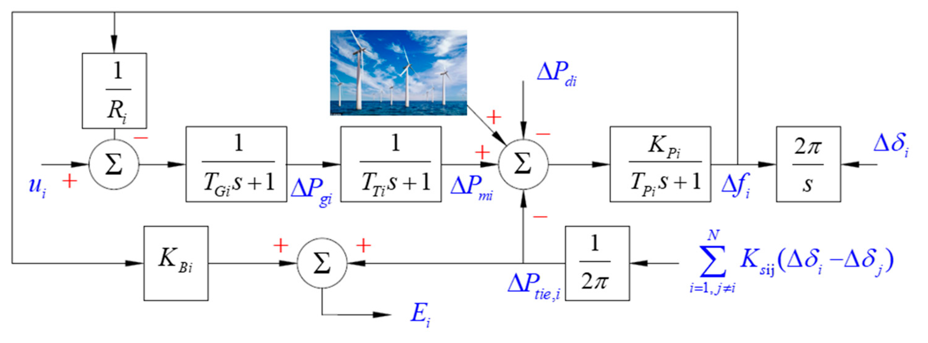
For the purpose of LFC, we first derive an MAIPS model. A power network with three areas is contemplated. Thus, areas 1 and 3 are integrated with a wind plant, whereas area 2 consists of a non-reheat turbine alone, as shown in Figure 1. In general, if ith area is considered, then the system is re-sketched as shown in Figure 2.
For simplicity, we have modeled the conventional and wind power networks separately. As we know, the conventional power system considered consists of a speed changer motor, governor, non-reheat turbine and generation. We model each component of the conventional MAIPS in the ith area, as displayed in Figure 2, in same way as [24,31]. Frequency change is made to be the output of the generator so that LFC can be achieved. Next, we determine the dynamic relations, which consist of a speed changer motor, a governor, a non-reheat turbine and a generator of the ith area model, as expressed by:
Δ f ˙ i ( t ) = K p i T P i Δ P m i ( t ) K p i T P i Δ P d i ( t ) + K p i T P i Δ P W i ( t ) 1 T P i Δ f i ( t ) K P i 2 π T P i i = 1 , j i N K ij { Δ δ i ( t ) Δ δ j ( t ) }
Δ P ˙ m i ( t ) = 1 T T i Δ P g i ( t ) 1 T T i Δ P m i ( t )
Δ P ˙ g i ( t ) = 1 R i T G i Δ f i ( t ) 1 T G i Δ P g i ( t ) + 1 T G i u i ( t )
Δ E ˙ i ( t ) = K E i K B i Δ f i ( t ) + K E i 2 π i = 1 , j i N K ij { Δ δ i ( t ) Δ δ j ( t ) }
Δ δ ˙ i ( t ) = 2 π Δ f i ( t )
where Δ f i ( t ) is the individual area frequency deviation, Δ P m i ( t ) is the mechanical power deviation of each area, Δ P g i ( t ) is each area turbine valve position deviation, Δ P d i ( t ) is each unit load deviation, R i is the individual area droop coefficient and K i j is the synchronization coefficient. Δ P W i ( t ) is the wind disturbance, Δ δ i ( t ) and Δ δ j ( t ) are small change in power angle, K B i and K E i are the frequency response coefficient. T P i , T G i and T T i are the subsystem parameters. Δ E ˙ i ( t ) is denoted as the area control error. The system state space form of ith area is shown as follows.
x ˙ i ( t ) = A i x i ( t ) + B i u i ( t ) + j = 1 j i N H i j x j ( t ) + F i Δ P d i ( t ) y i ( t ) = C i x i ( t )
The system matrices A i , B i , F i , H i j in the state space model are given below:
A i = [ 1 T P i K P i T P i 0 0 K P i 2 π T P i i = 1 , j i N K ij 0 1 T T i 1 T T i 0 0 1 R i T G i 0 1 T G i 0 0 K B i K E i 0 0 0 K E i 2 π i = 1 , j i N K ij 2 π 0 0 0 0 ] , H i j = [ 0 0 0 0 K P i 2 π T P i i = 1 , j i N K ij 0 0 0 0 0 0 0 0 0 0 0 0 0 0 K E i 2 π i = 1 , j i N K ij 0 0 0 0 0 ] , B i = [ 0 0 1 T G i 0 0 ] and F i = [ 1 2 H i 1 2 H i 0 0 0 0 0 0 0 0 ]
x i ( t ) = [ Δ f i ( t ) Δ P m i ( t ) Δ P g i ( t ) E i ( t ) Δ δ i ( t ) ] T represent the state variables in the state space model. u i ( t ) R m is the control input. Δ P d i ( t ) is the load uncertainty.
The model of the wind farm in the ith area is further discussed in the next section.

3. Wind Plant Model

A typical variable speed wind turbine generator system (VS-WTGS) is evaluated. For the VS-WTGSs, the wind power generates mechanical torque via the turbine generator shaft; thus, electrical torque is produced. The mechanical system acceleration, deceleration or constant speed depend on the change in mechanical and electrical torque. Thus, the net power output is related to the mechanical power.
Building the dynamic equations of the wind plant is based on the relationship of mechanical output power and wind velocity. The output power is therefore given as [35]
P m = C p ( λ , β ) 1 2 ρ A V 3 w i n d
where P m is the turbine mechanical output (W), C p is the turbine performance coefficient, λ is the tip speed ratio, β is the pitch angle of the blade (deg), ρ is the air density ( k g / m 3 ), A is the turbine swept area ( m 2 ) and V w i n d is the wind speed (m/s).
The tip speed ratio ( λ )
λ = ω r R r V w
where R r and ω r are radius and spin speed of the wind plant, respectively.
Performance coefficient ( C p ) of the turbine is given by.
C p ( λ , β ) = c 1 ( c 2 λ i c 3 β c 4 ) e c 5 λ i + c 6 λ
with
1 λ i = 1 λ + 0.08 β 0.035 β 3 + 1
where the coefficients c 1 to c 6 are dependent on the wind plant.
Finally, we can present the equation of the wind plant via a per-unit (p.u) system, as given below.
P m _ p u = k p × C p _ p u × V w i n d _ p u 3
P m _ p u is the mechanical power in per unit, k p 1 is the amplified power factor, C p _ p u is the power factor and V w i n d _ p u is the wind speed.
To design the new LFC for the MAIPS, we derive the following basic assumption. A lemma is also adopted to accompany the progress of the work.
Assumption 1.
Load uncertainty Δ P d i ( t ) and the differential of Δ P d i ( t ) is bounded such that Δ P d i ( t ) τ i and Δ P ˙ d i ( t ) τ ¯ i , where γ i and γ ¯ i are known scalars and . is a matrix norm.
Assumption 2.
The eigenvalues of the matrix A i T i C i can be chosen arbitrarily by appropriate choice of the observer gain T i when the pair [ A i , C i ] is observable.
Lemma 1
[24]. Let X and Y be a real matrix of suitable dimension then, for any scalar μ > 0 , the below matrix inequality holds:
X T Y + Y T X μ X T X + μ 1 Y T Y .

4. State Observer Based on Sliding Mode Control Strategies

4.1. Multi-Area Power System State Observer Design

This part, we considered the fact that the power network state variables are difficult to measure. Therefore, the state observer technique is applied. The original internal state of (6) is then estimated by the state observer using the experience of the output and input; therefore, the observer is designed as follows.
z ˙ i ( t ) = A i z i ( t ) + B i u i ( t ) + j = 1 j i N H i j z j ( t ) + T i ( y i ( t ) n i ( t ) ) n i ( t ) = C i z i
where z i is the estate of x i and T i is a matrix gain, which is selected to ensure that the continuous-time dynamics error converges to zero faster. y i ( t ) is the output signal of the power system and n i ( t ) is the state observer output, respectively.

4.2. Stability Analysis of Whole System in Sliding Mode Dynamic

The new SMC is designed with a better sliding surface for sliding variables to rapidly reach the surface and remain thereon. The sliding surface is therefore given below
σ i [ z i ( t ) ] = L i z i ( t ) 0 t L i ( A i B i J i ) z i ( τ ) d τ
where L i is a constant matrix and J i is the design matrix. Matrix L i is selected to guarantee that the matrix L i B i is invertible. The design matrix J i R m i × n i is given, satisfying the non-linearity condition
Re [ λ max ( A i B i J i ) ] < 0
For the continuous system observability rule, the estimation error defined by e i ( t ) = x i ( t ) z i ( t ) must satisfy the below equation
e ˙ i = ( A i T i C i ) e i + j = 1 j i N H i j e j + F i Δ P d i ( t )
If we take the derivative of (13) with respect to time, we therefore obtain
σ ˙ i [ z i ( t ) ] = L i [ A i z i ( t ) +   B i u i ( t ) + j = 1 j i N H i j z j ( t ) + T i ( y i n i ) ]   L i ( A i B i J i ) z i ( t )
Setting σ ˙ ( t ) = σ ( t ) = 0 , we can see that the equivalent control signal is as below
u i e q ( t ) = ( L i B i ) 1 [ L i A i z i ( t ) + j = 1 j i N L i H i j z j ( t ) + L i T i ( y i n i ) ] L i ( A i B i J i ) z i ( t ) ] = ( L i B i ) 1 [ L i B i J i z i ( t ) + L i T i ( y i n i ) + j = 1 j i N L i H i j z j ( t ) ]
Substituting u ( t ) into (6) yields the sliding motion:
x ˙ i ( t ) = A i x i ( t ) B i J i z i ( t ) B i ( L i B i ) 1 L i T i ( y i n i ) j = 1 j i N B i ( L i B i ) 1 L i H i j z j ( t ) + j = 1 j i N H i j x j ( t ) + F i Δ P d i ( t ) = ( A i B i J i ) x i ( t ) + ( B i J i B i ( L i B i ) 1 L i T i C i ) e i ( t ) + j = 1 j i N [ H i j B i ( L i B i ) 1 L i H i j ] x j ( t ) + j = 1 j i N B i ( L i B i ) 1 L i H i j e j ( t ) + F i Δ P d i ( t )
Combining system (6) and error system (18), the closed-loop system is written as
[ x ˙ i e ˙ i ] = [ A i B i J i Φ i 0 A i T i C i ] [ x i e i ] + j = 1 j i N [ H i j Λ i H i j Λ i H i j 0 H i j ] [ x j e j ] + [ F i Δ P d i ( t ) F i Δ P d i ( t ) ]
where Φ i = B i J i B i ( L i B i ) 1 L i T i C i and Λ i = B i ( L i B i ) 1 L i .
Equation (19) provides the condition that the MAIPS in the sliding surface is stable if the sliding motion (19) is stable and the observability condition holds following assumption 2. Therefore, the sliding motion (19) is also made Hurwitz, so the observer error e ( t ) 0   when t . To prove the above condition, we postulate a theorem as follows.
Theorem 1.
The sliding motion (19) is asymptotically stable, if there exist symmetric positive definite matrices P i , Q i , i = 1 ,   2 ,   .   .   . N and positive scalars λ i , ρ i , γ ^ i and γ ¯ i so that the below linear matrix inequality is feasible
[ Χ i + j = 1 j i N [ λ ¯ j ( H j i Λ j H j i ) T ( H j i Λ j H j i ) ] P i Φ i P i P i F i 0 0 Φ i T P i Χ ¯ i + j = 1 j i N [ λ ˜ j 1 H j i T H j i ] + j = 1 j i N [ λ ^ j ( Λ j H j i ) T Λ j H j i ] 0 0 Q i F i T Q i P i 0 λ i 1 0 0 0 F i T P i 0 0 γ ^ i 1 0 0 0 Q i 0 0 ρ i 1 0 0 F i T Q i 0 0 0 ν i 1 ] < 0
where Χ i = P i ( A i B i J i ) + ( A i B i J i ) T P i and Χ ¯ i = Q i ( A i T i C i ) + ( A i T i C i ) T Q i .
Proof. 
In the analysis of the stability of the sliding motion (19), we choose the below Lyapunov function
V = i = 1 N [ x i e i ] T [ P i 0 0 Q i ] [ x i e i ]
where P i > 0 and Q i > 0 satisfy (20) for i = 1 ,   2 , N . By getting the time derivative along the system state trajectory of MAIPS, we have
V ˙ = i = 1 N [ x ˙ i e ˙ i ] T [ P i 0 0 Q i ] [ x i e i ] + i = 1 N [ x i e i ] T [ P i 0 0 Q i ] [ x ˙ i e ˙ i ] = i = 1 N { [ x i e i ] T [ ( A i B i J i ) T P i 0 Φ i T P i ( A i T i C i ) T Q i ] [ x i e i ] + j = 1 j i N [ x j e j ] T [ ( H i j Λ i H i j ) T P i 0 ( Λ i H i j ) T P i H i j T Q i ] [ x i e i ] + [ ( F i Δ P d i ) T P i ( F i Δ P d i ) T Q i ] [ x i e i ] } + i = 1 N { [ x i e i ] T [ P i ( A i B i J i ) P i Φ i 0 Q i ( A i T i C i ) ] [ x i e i ] + j = 1 j i N [ x i e i ] T [ P i ( H i j Λ i H i j ) P i Λ i H i j 0 Q i H i j ] [ x j e j ] + [ x i e i ] T [ P i F i Δ P d i Q i F i Δ P d i ] }
= i = 1 N { [ x i e i ] T [ P i ( A i B i J i ) + ( A i B i J i ) T P i P i Φ i Φ i T P i Q i ( A i T i C i ) + ( A i T i C i ) T Q i ] [ x i e i ] + i = 1 N j = 1 j i N [ x j T ( H i j Λ i H i j ) T P i x i + x i T P i ( H i j Λ i H i j ) x j + e j T ( Λ i H i j ) T P i x i + x i T P i Λ i H i j e j ] + i = 1 N j = 1 j i N ( e i T Q i H i j e j + e j T H i j T Q i e i ) + i = 1 N [ e i T Q i F i Δ P d i + x i T P i F i Δ P d i + ( F i Δ P d i ) T P i x i + ( F i Δ P d i ) T Q i e i ]
Applying Lemma 1 to Equation (22), we have
V ˙ i = 1 N { [ x i e i ] T [ P i ( A i B i J i ) + ( A i B i J i ) T P i P i Φ i Φ i T P i Q i ( A i T i C i ) + ( A i T i C i ) T Q i ] [ x i e i ] + i = 1 N j = 1 j i N [ λ ¯ i x j T ( H i j Λ i H i j ) T ( H i j Λ i H i j ) x j + λ ¯ i 1 x i T P i P i x i + λ ^ i e j T ( Λ i H i j ) T Λ i H i j e j + λ ^ i 1 x i T P i P i x i ] + i = 1 N j = 1 j i N ( λ ˜ i e i T Q i Q i e i + λ ˜ i 1 e j T H i j T H i j e j ) + i = 1 N [ ν i e i T Q i F i F i T Q i e i + ν i 1 Δ P d i T Δ P d i + γ ˜ i x i T P i F i F i T P i x i + γ ˜ i 1 Δ P d i T Δ P d i i ]
Since i = 1 N j = 1 j i N λ ¯ i x j T ( H i j Λ i H i j ) T ( H i j Λ i H i j ) x j = i = 1 N j = 1 j i N λ ¯ j x i T ( H j i Λ j H j i ) T ( H j i Λ j H j i ) x i i = 1 N j = 1 j i N λ ^ i e j T ( Λ i H i i ) T Λ i H i j e j = i = 1 N j = 1 j i N λ ^ j e i T ( Λ j H j i ) T Λ j H j i e i and i = 1 N j = 1 j i N λ ˜ i 1 e j T H i j T H i j e j = i = 1 N j = 1 j i N λ ˜ j 1 e i T H j i T H j i e i , we achieve
V ˙ i = 1 N { [ x i e i ] T [ P i ( A i B i J i ) + ( A i B i J i ) T P i P i Φ i Φ i T P i Q i ( A i T i C i ) + ( A i T i C i ) T Q i ] [ x i e i ] + i = 1 N j = 1 j i N [ λ ¯ j x i T ( H j i Λ j H j i ) T ( H j i Λ j H j i ) x i + λ ¯ i 1 x i T P i P i x i + λ ^ j e i T ( Λ j H j i ) T Λ j H j i e i + λ ^ i 1 x i T P i P i x i ] + i = 1 N j = 1 j i N ( λ ˜ i e i T Q i Q i e i + λ ˜ j 1 e i T H j i T H j i e i ) + i = 1 N [ ν i e i T Q i F i F i T Q i e i + ν i 1 Δ P d i T Δ P d i + γ ˜ i x i T P i F i F i T P i x i + γ ˜ i 1 Δ P d i T Δ P d i i ] = i = 1 N { [ x i e i ] T [ Χ i + λ i P i P i + γ ˜ i P i F i F i T P i + j = 1 j i N [ λ ¯ j ( H j i Λ j H j i ) T ( H j i Λ j H j i ) ] P i Φ i Φ i T P i Χ ¯ i + ρ i Q i Q i + ν i Q i F i F i T Q i + j = 1 j i N [ λ ˜ j 1 H j i T H j i ] + j = 1 j i N [ λ ^ j ( Λ j H j i ) T Λ j H j i ] ] [ x i e i ] } + i = 1 N [ ( ν i 1 + γ ˜ i 1 ) Δ P d i T Δ P d i ]
where λ i = ( N 1 ) ( λ ¯ i 1 + λ ^ i 1 ) , ρ i = λ ˜ i ( N 1 ) , Χ i = P i ( A i B i J i ) + ( A i B i J i ) T P i and Χ ¯ i = Q i ( A i T i C i ) + ( A i T i C i ) T Q i .
In addition, using the Schur complement, the LMI (20) is equivalent to the below inequality
Ω i = [ Χ i + λ i P i P i + γ ˜ i P i F i F i T P i + j = 1 j i N [ ν j ( H j i Λ j H j i ) T ( H j i Λ j H j i ) ] P i Φ i Φ i T P i Χ ¯ i + ρ i Q i Q i + ν i Q i F i F i T Q i + j = 1 j i N [ λ ˜ j 1 H j i T H j i ] + j = 1 j i N [ λ ^ j ( Λ j H j i ) T Λ j H j i ] ] > 0
According to Equations (24) and (25), we obtain
V ˙ i = 1 N ( λ min ( Ω i ) x ^ i ( t ) 2 + μ i )
where the constant value μ i = i = 1 N [ ( ν i 1 + γ ˜ i 1 ) τ i 2 ] and the eigenvalue λ min ( Ω i ) > 0 . Therefore, V ˙ < 0 is achieved with x ^ i ( t ) > μ i λ min ( Ω i ) . Hence, the sliding motion (19) is asymptotically stable. □

4.3. Decentralized State Estimator Feedback Integral Sliding Mode Control (DSEFISMC) Design

Previously, we designed the integral surface and proved the power system asymptotically stability in the sliding motion. Next, a continuous second-order DSEFISMC law is developed to reduce the chattering inherent in the first-order design. We start by defining the second-order sliding manifold S i [ z i ( t ) ] such that the estimated system state trajectories are forcefully driven to zero asymptotically, which is given as
S i [ z i ( t ) ] = σ ˙ i [ z i ( t ) ] + ε i σ i [ z i ( t ) ]
and
S ˙ i [ z i ( t ) ] = σ ¨ i [ z i ( t ) ] + ε i σ ˙ i [ z i ( t ) ]
where ε i > 0 is a positive constant. Using Equation (16) yields
S ˙ i [ z i ( t ) ] = L i [ A i z ˙ i ( t ) + B i u ˙ i ( t ) + j = 1 j i N H i j z ˙ j ( t ) + T i ( y ˙ i ( t ) n ˙ i ( t ) ) ] L i ( A i B i J i ) z ˙ i ( t ) + ε i σ ˙ i [ z i ( t ) ]
Based on the definition of the sliding surface and sliding manifold, the continuous DSEFISMC law for the MAIPS is known as follows
u ˙ i ( t ) = ( L i B i ) 1 { L i B i J i z ˙ i ( t ) + ε i σ ˙ i [ z i ( t ) ] + j = 1 j i N L j H j i z ˙ i ( t ) + L i T i ( y ˙ i ( t ) n ˙ i ( t ) ) δ i s a t ( S i [ z i ( t ) ] ) }
We propound a theorem to demonstrate the reachability of the estimated system state trajectories to the manifold in the following.
Theorem 2.
Consider Equation (6) with the continuous DSEFISMC law (30). Then, system state trajectory is directed towards the sliding manifold S i [ z i ( t ) ] and once the trajectory hits the sliding manifold S i [ z i ( t ) ] it remains on the sliding manifold thereafter.
Proof. 
A Lyapunov function is therefore, obtained:
V ¯ ( t ) = i = 1 N S i [ z i ( t ) ]
Now using the time derivative of V ¯ ( t ) yields
V ¯ ˙ = i = 1 N S i T [ z i ( t ) ] S i [ z i ( t ) ] S ˙ i [ z i ( t ) ] = i = 1 N S i T [ z i ( t ) ] S i [ z i ( t ) ] { L i [ A i z ˙ i ( t ) + B i u ˙ i ( t ) + j = 1 j i N H i j z ˙ j ( t ) + T i ( y ˙ i ( t ) n ˙ i ( t ) ) ] L i ( A i B i J i ) z ˙ i ( t ) + ε i σ ˙ i [ z i ( t ) ] } = i = 1 N S i T [ z i ( t ) ] S i [ z i ( t ) ] { L i B i J i z ˙ i ( t ) + ε i σ ˙ i [ z i ( t ) ] + j = 1 j i N L i H i j z ˙ i ( t ) + L i T i ( y ˙ i ( t ) n ˙ i ( t ) ) } + i = 1 N S i T [ z i ( t ) ] S i [ z i ( t ) ] L i B i u ˙ i ( t )
Using the DSEFISMC law (30), Equation (32) yields
V ¯ ˙ i = 1 N δ i
The above Equation implies that the system state trajectories reach the sliding manifold S i [ z i ( t ) ] and stay on it thereafter. □

5. Result Discussions

In this segment, we simulate the performance of the MAIPS with the proposed state observer based on sliding mode control (SOboSMC) and the results are compared and discussed with the load frequency double integral sliding mode controller given in [23] and the sliding mode controller in combination with the extended state observer in [34].

5.1. Simulation 1

In this simulation, the test was carried out in three cases and the parameters of the power network considered were the same as those in [23]. The one-line diagram of the MAIPS integrated with the wind plant is shown in Figure 3.
Case 1. In this case, the initial values of the MAIPS are assumed to be nominal values at time zero. The load disturbances of the areas 1, 2 and 3 are given as Δ P d 1 = 0.01   p . u .   M W , Δ P d 2 = 0.015   p . u .   M W , Δ P d 3 = 0.02   p . u .   M W at 1 s and the wind variations are neglected.
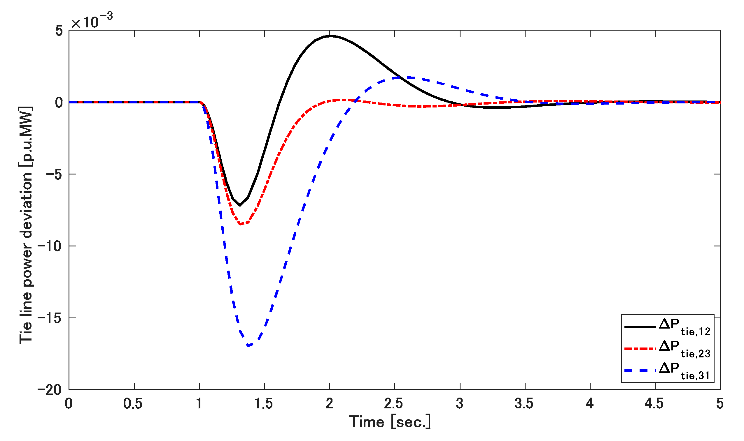
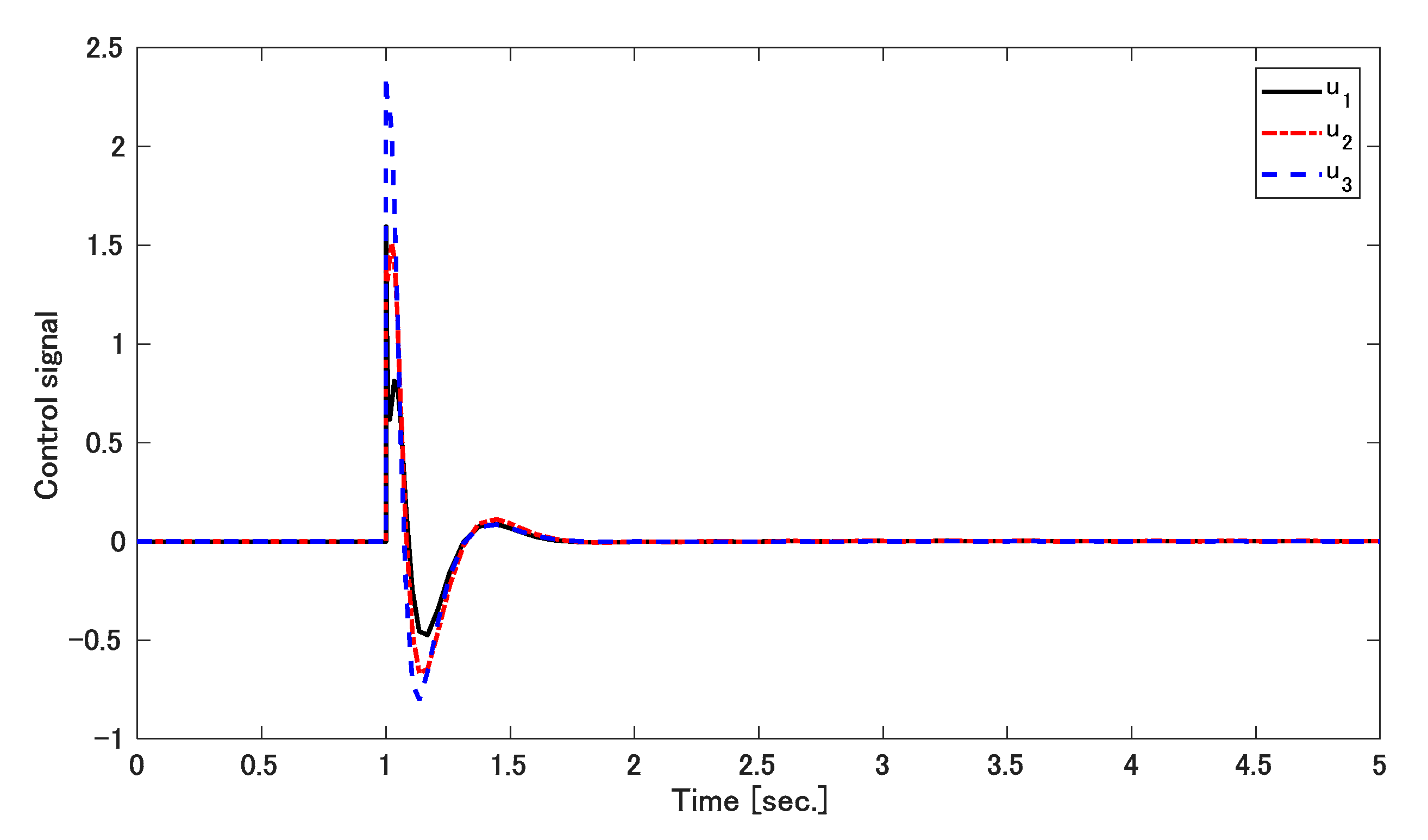
The incremental frequency is displayed in Figure 4 and the tie-line power deviation is shown in Figure 5, whereas the control signal is given in Figure 6.
Remark 1.
Under the assumed initial conditions of the MAIPS, the proposed SOboSMC acted quickly to converge the frequency error to zero at 3 s, with a maximum overshoot of 0.005 Hz as compared to the 6-s settling time and maximum overshoot of 0.08 Hz seen in [23]. This validates that the MAIPS performance is better when using the proposed SOboSMC.
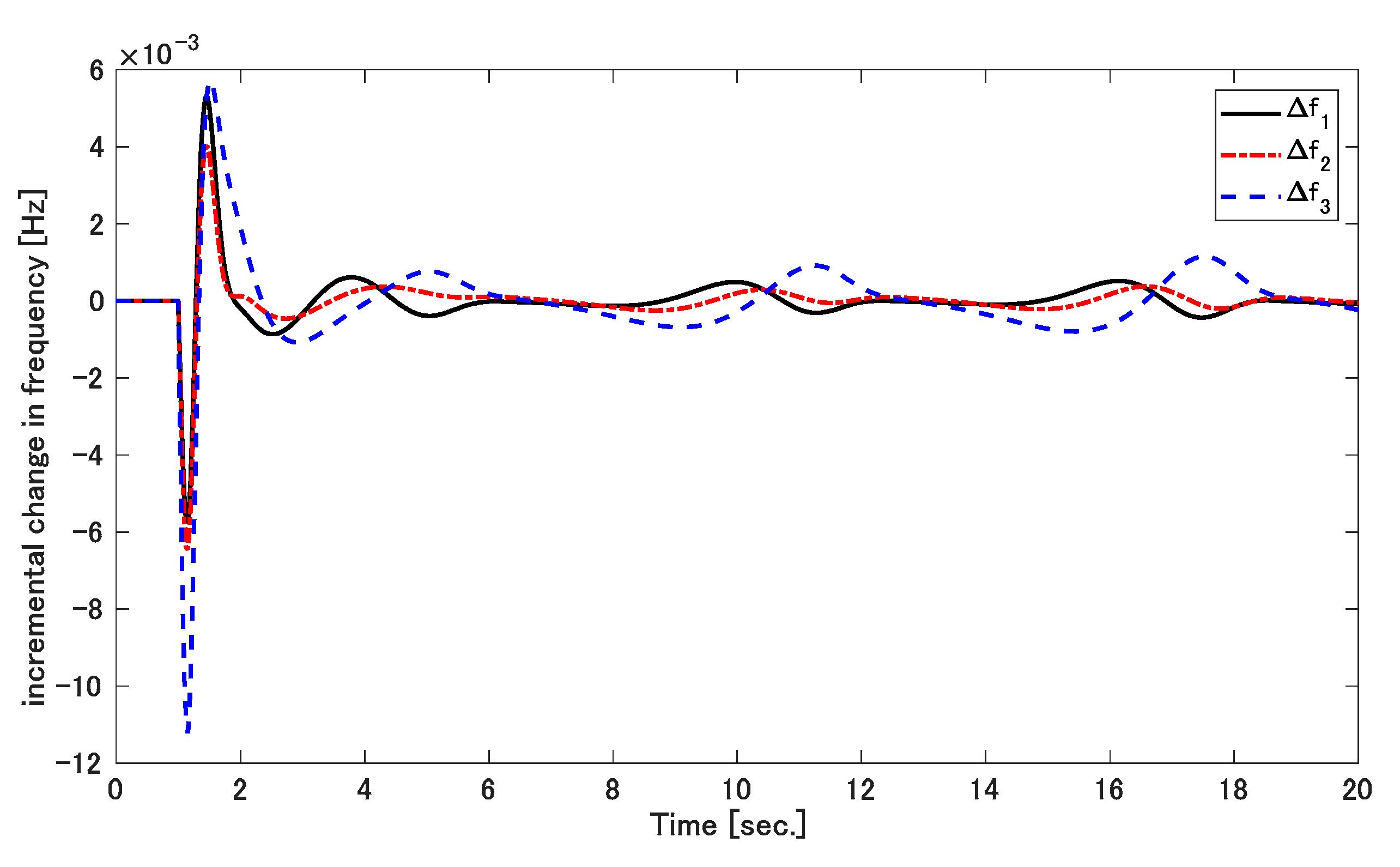
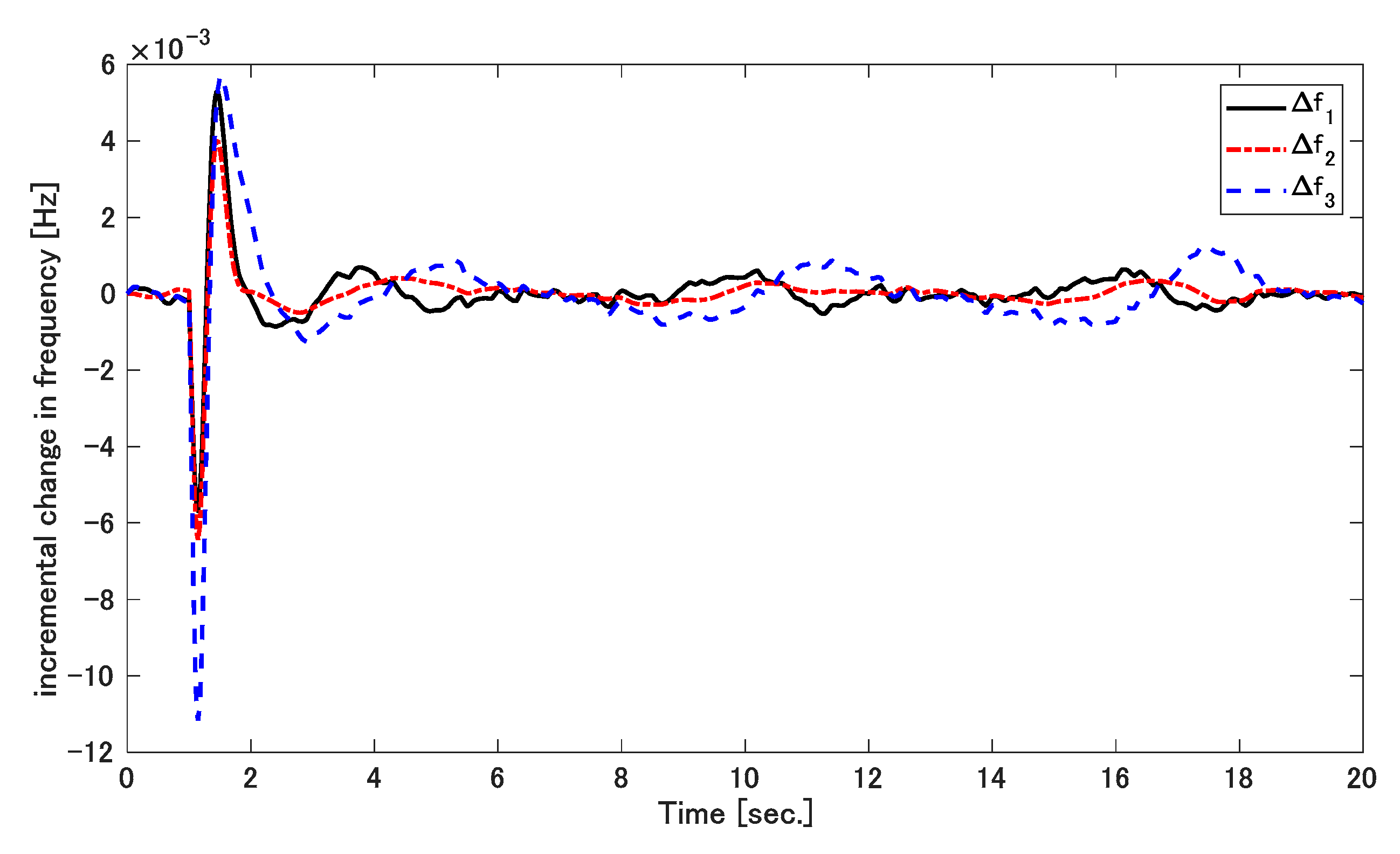
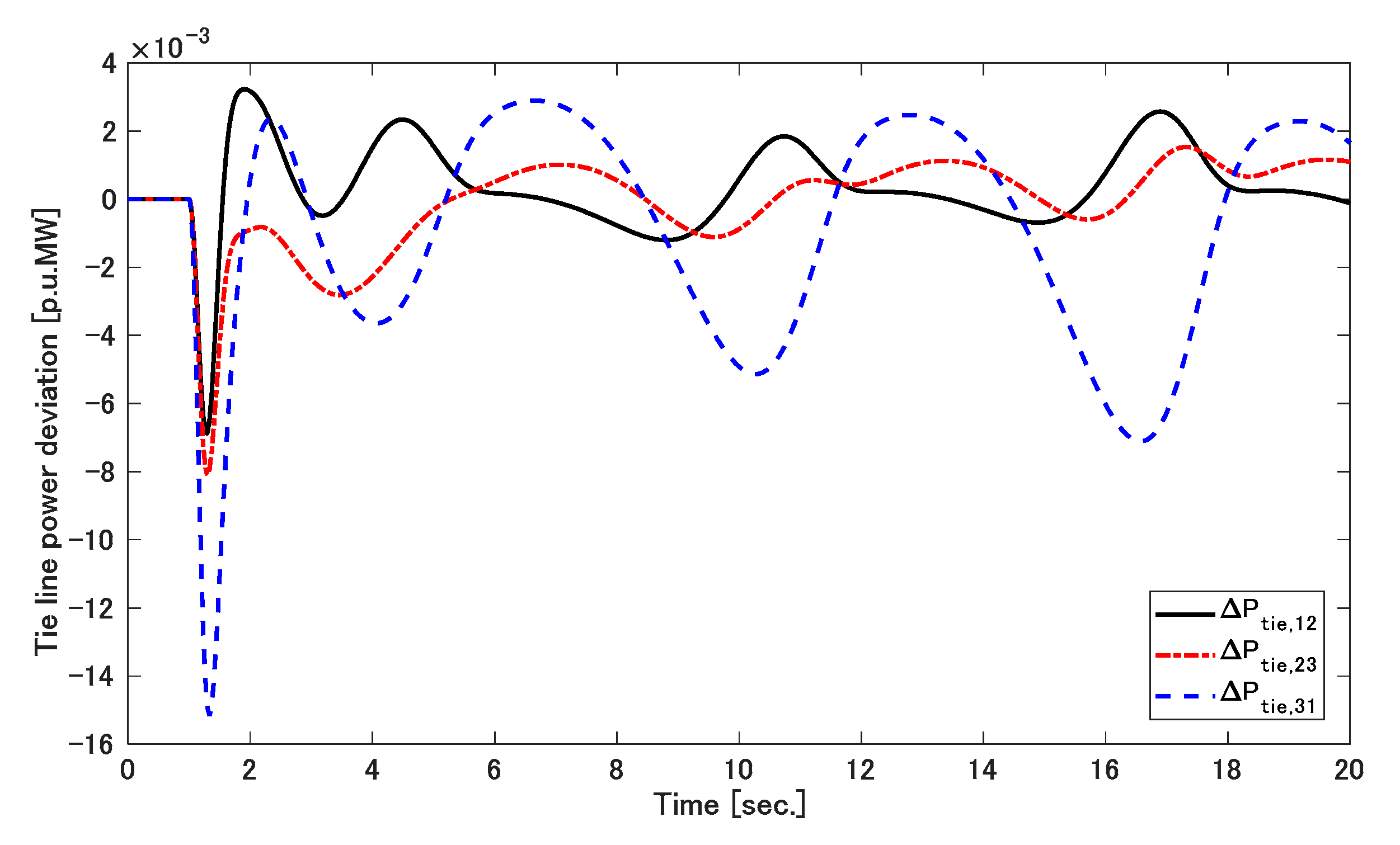
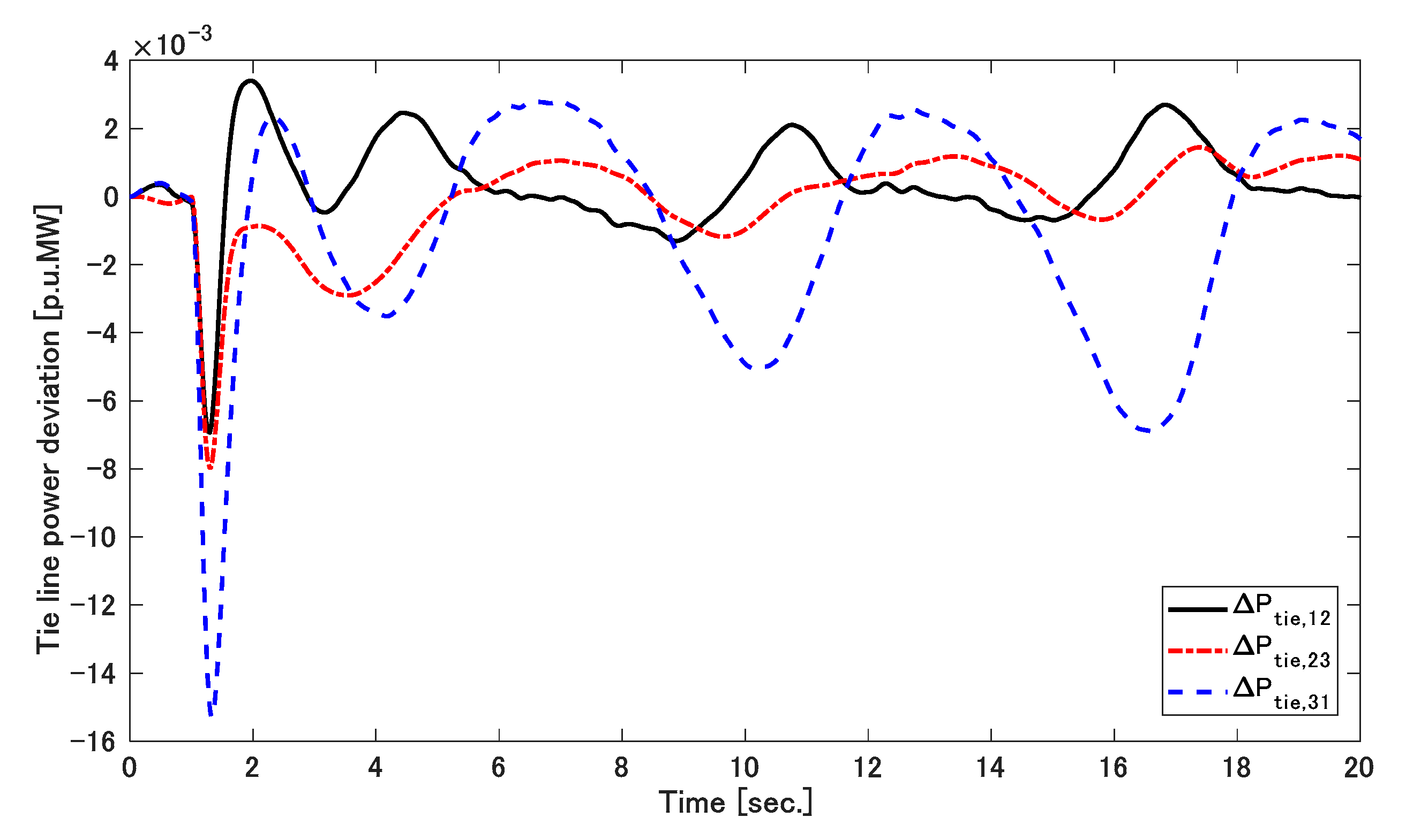
Case 2. This simulation was done with the MAIPS with and without wind turbines. The load disturbances of the areas 1, 2 and 3 were assumed to be the same as those in case 1 and [23]. The parametric uncertainty is considered in the form of matched uncertainty A i , which is expressed as
Δ A 1 = [ 0 0 0 0 0 0 0 0 0 0 2.26 cos ( t ) 2 cos ( t ) 2.604 cos ( t ) 3 cos ( t ) 0 0 0 0 0 0 0 0 0 0 0 ]   where   Δ A 1 = Δ A 2 = Δ A 3 .
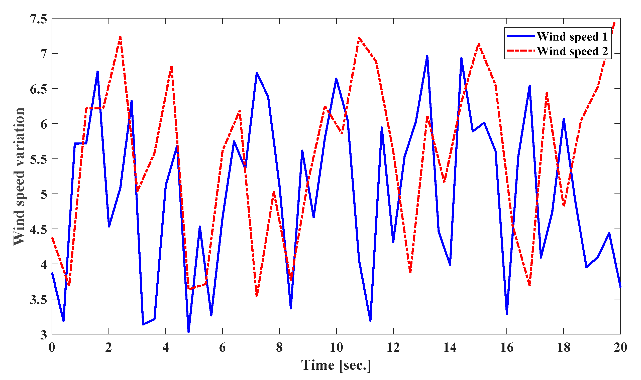
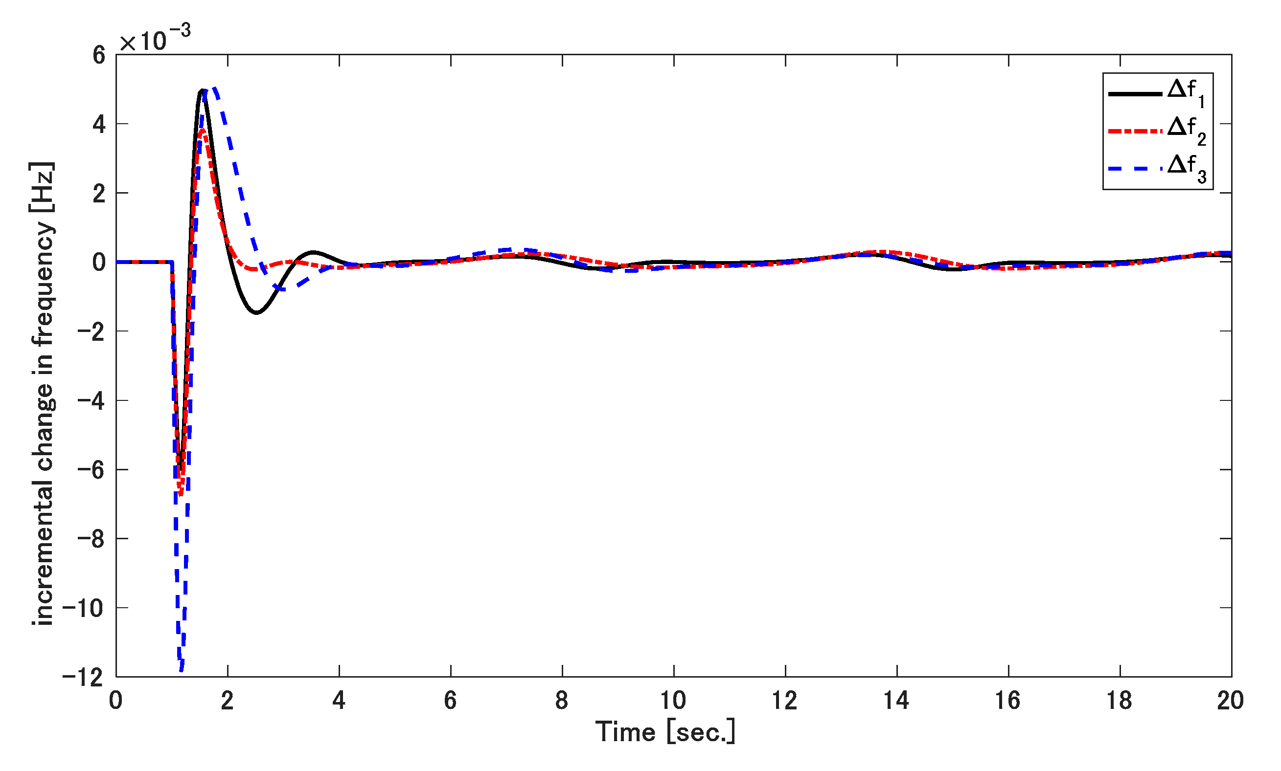
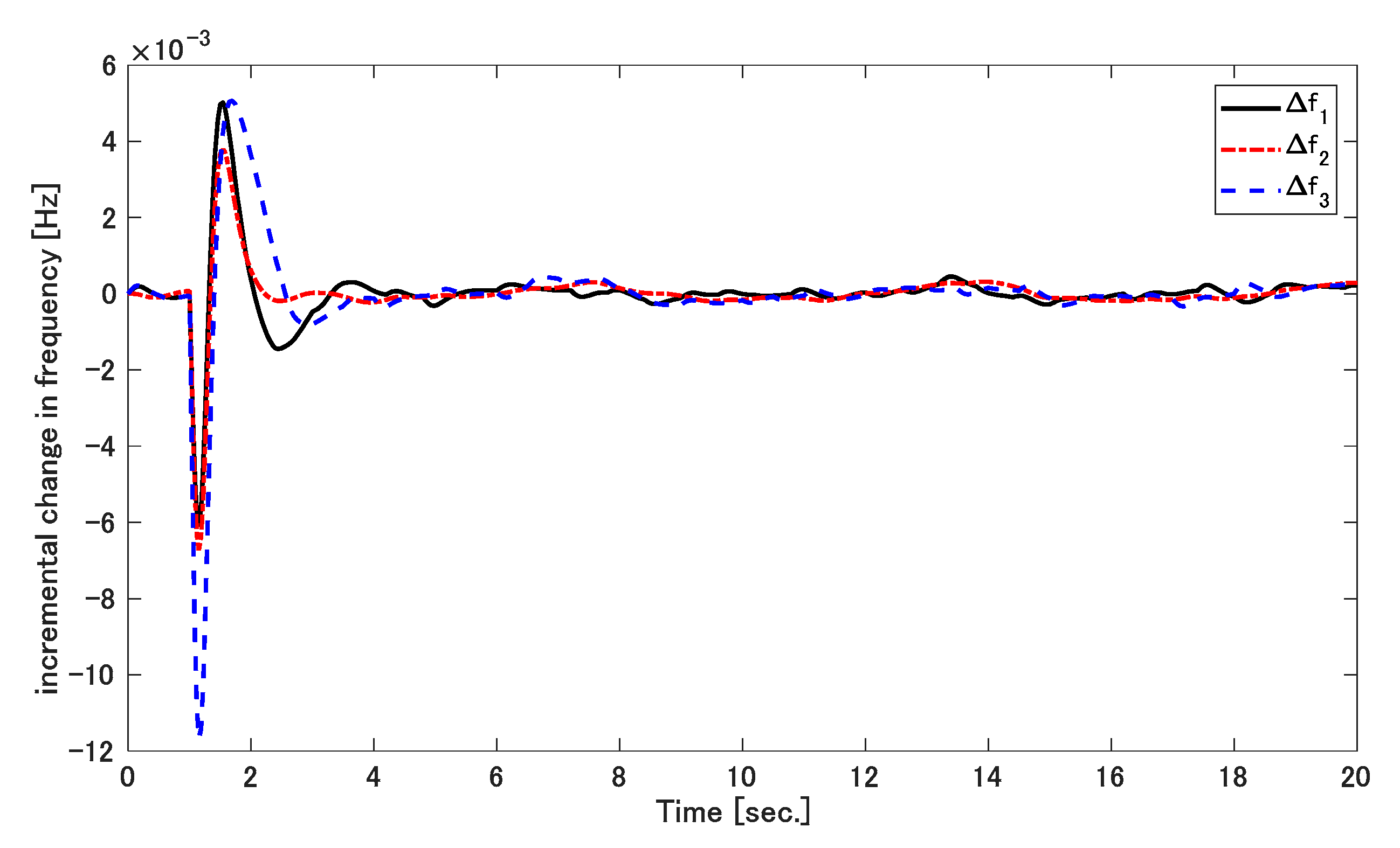
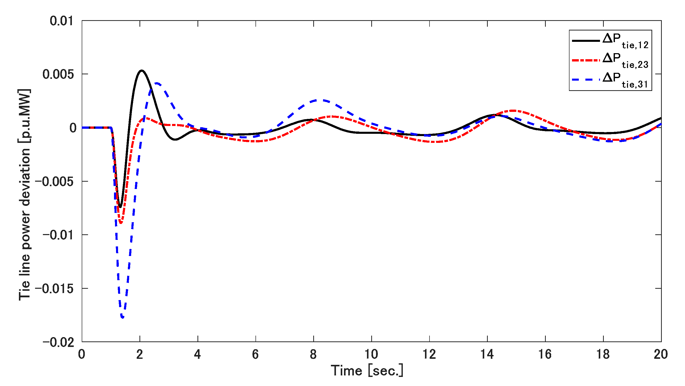
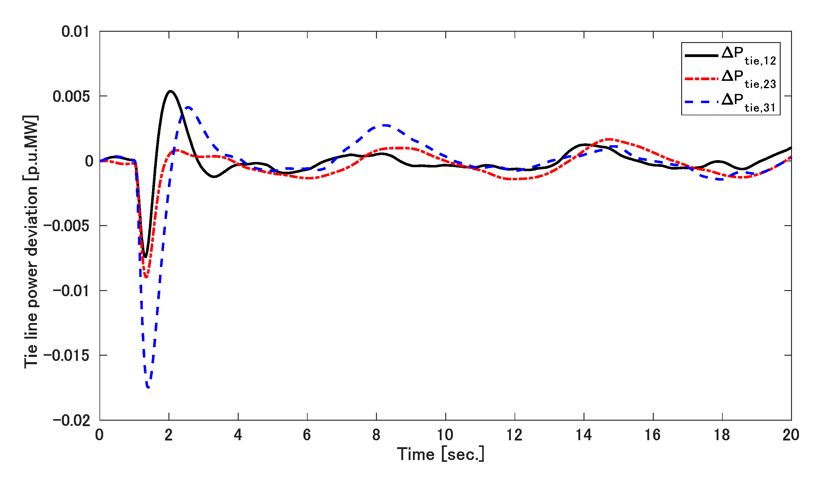
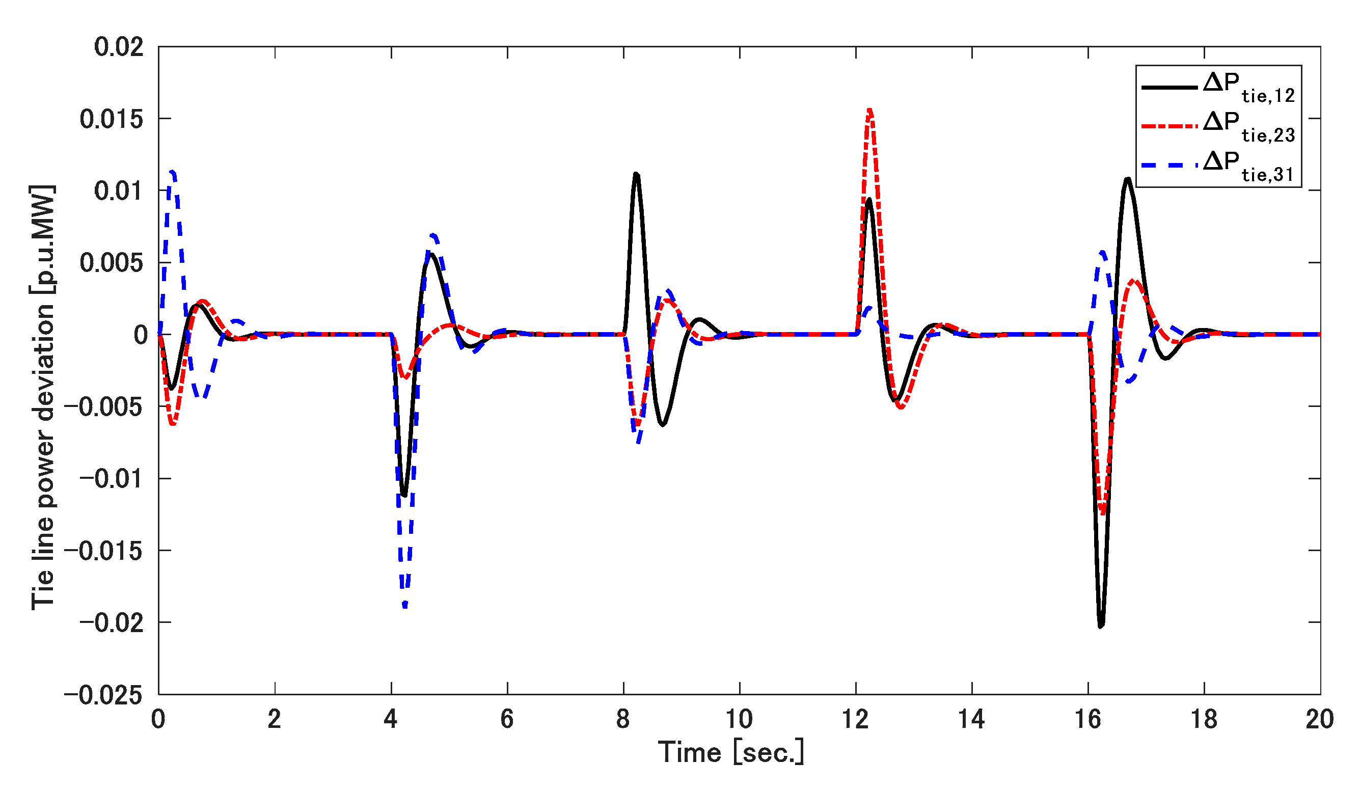
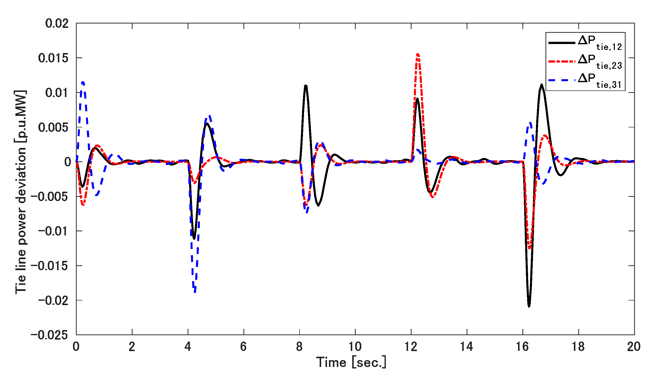
The wind variation is shown in Figure 7. The frequency error with and without the wind plant can be seen in Figure 8 and Figure 9, whereas the tie-line power error with and without the wind farm are shown in Figure 10 and Figure 11. For the MAIPS without wind farms, the response of the power network is better, pertaining to overshoot and settling time, and is also chattering-free in comparison with the design presented in [23]. Once more, the frequency transient is kept within the operational safety range, which is ±0.2 Hz for the safety of the power system frequency [36]. Therefore, the proposed approach shows good control performance for the LFC of an MAIPS with load disturbances, parameter uncertainties and wind variations, without the loss of control accuracy.
Remark 2.
The LFC for the MAIPS with load disturbance and matched uncertainty can be seen in [23]. However, the above approach cannot be applied to an MAIPS with a wind turbine; therefore, this new approach is a better choice to handle the LFC in the MAIPS integrated with renewable plants.
Case 3. The load change and the wind variation were the same as those in case 2. The parametric uncertainty was in the form of mismatched uncertainty in the system matrix and in the interconnected matrix [23].
Δ A 1 = [ 0 Δ f 1 0 0 0 sin ( t ) 0 0 0 0 0 0 cos ( t ) cos ( t ) 0 0 0 0 0 cos ( t ) cos ( t ) 0 0 0 0 ]   and   Δ H 12 = [ 0 0 0 0 0.178 cos ( t ) 0 0 0 0 0 0 0 0 0 0 0 0 0 0 0.296 sin ( t ) 0 0 0 0 0 ]
We also assumed that Δ H 2 = Δ H 3 = Δ H 1 and Δ A 2 = Δ A 3 = Δ A 1 .
Figure 12, Figure 13, Figure 14 and Figure 15 represent the frequency and tie-line power error of the MAIPS with and without a wind turbine under the mismatched uncertainties, coupled with load disturbance. The results indicate that the new approach is highly robust against power system uncertainties and wind variation in comparison with [23].
Remark 3.
Even with load disturbances, wind variation and matched and mismatched parametric uncertainties, the results from Table 1 show that the proposed SOboSMC preserves the frequency of the MAIPS, which is better in terms of overshoot and settling time in comparison with [23]. Thus, the new controller is proven to be a preferred choice to cope with a power system with the above conditions. Unlike the approach given in [23], the system state variables are not required to be measured, so the proposed SOboSMC is much easier to apply to a large power network. The proposed SOboSMC is also intended to be applied to imperfect systems, which are mentioned in [37].

5.2. Simulation 2

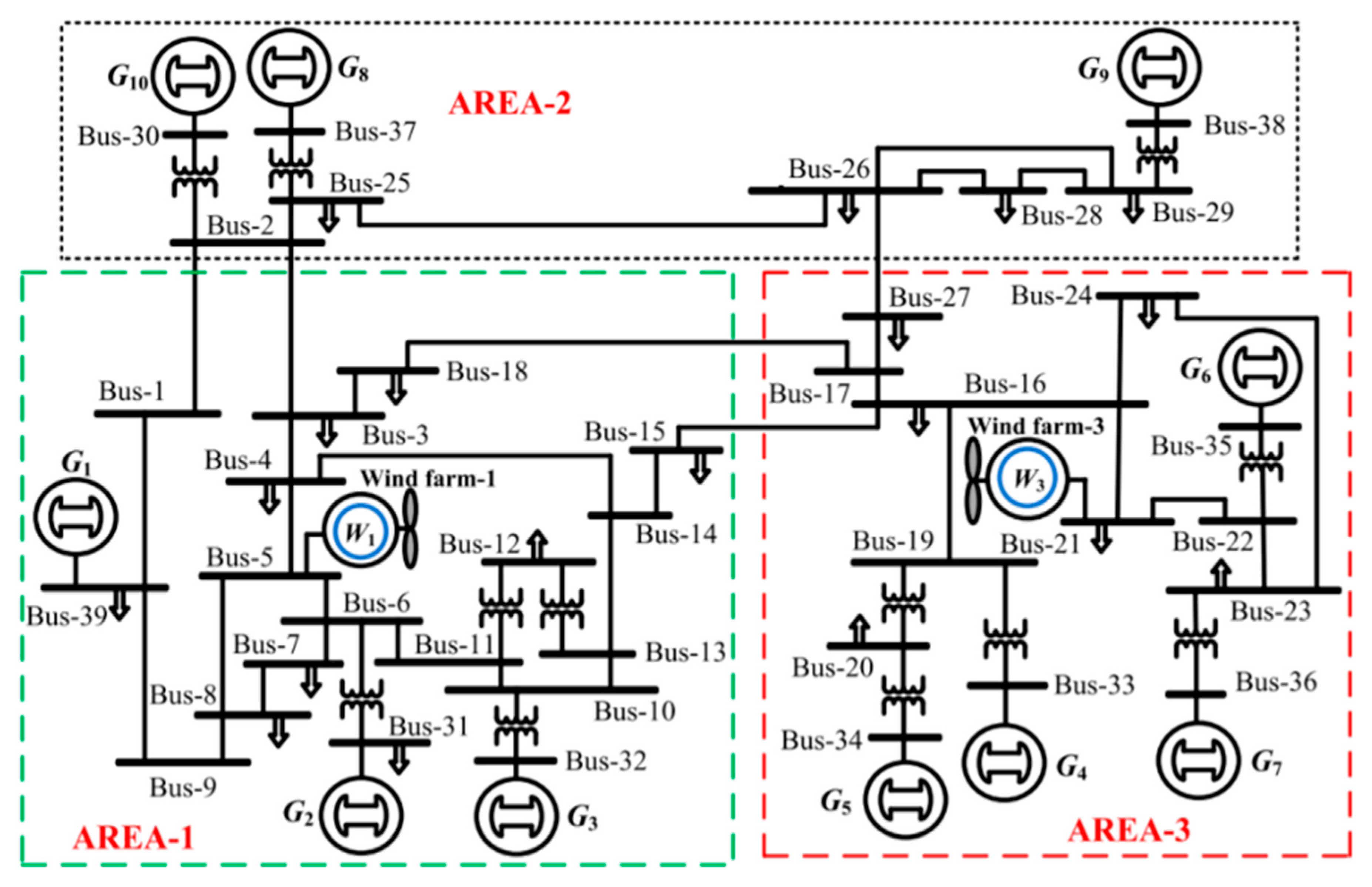
In other to test the proposed SOBoSMC for the real MAIPS, a New England 39 bus power system (PS) was used. The configuration and parameters of the power system in this simulation were taken from [34].
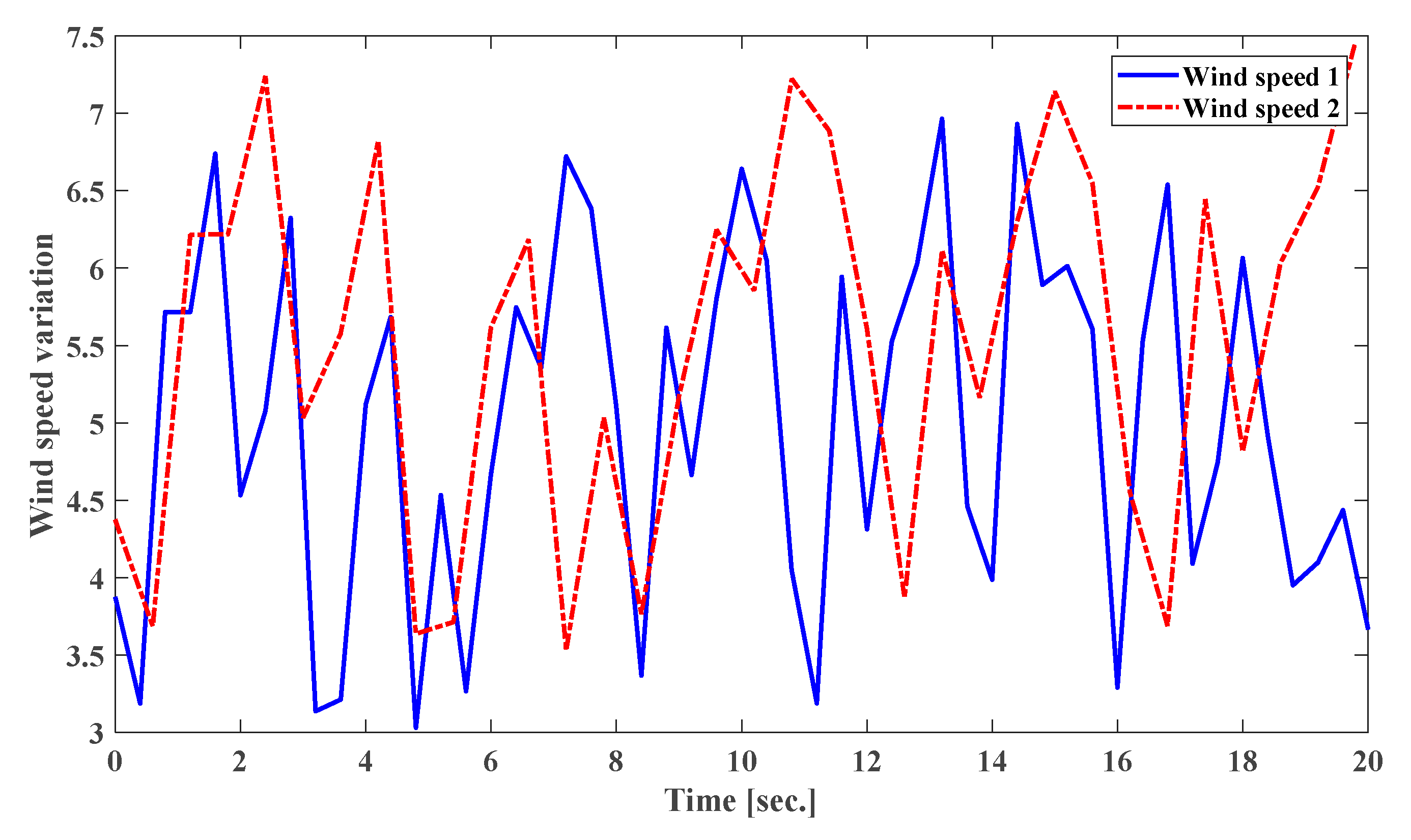
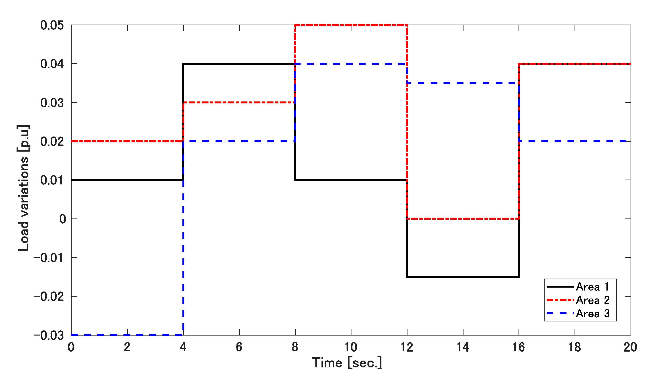
In addition, the importance of integrating renewable energy with MAIPSs has been discussed in [32]. Therefore, we considered integrating wind energy with area 1 at bus 5 and area 3 at bus 21 of the New England 39 bus PS. A single line diagram of the New England 39 bus PS integrated with a wind plant is shown in Figure 16. The proposed SOBoSMC was tested for the LFC of the New England PS with and without wind plants. The wind variation was assumed as shown in Figure 17 and the load disturbance was applied for the MAIPS as shown in Figure 18. On the other hand, the SMC combined with the disturbance observer was used to increase the damping ratio for the LFC of the New England PS under random loads, as given in [34]. However, the stability of the frequency and tie-line power of the PS were attained without wind variation and the controller was required to measure all the system state variables. IN addition, an observer-based SMC used for the LFC of a New England PS was also seen in [32]. However, that controller suffered from chattering problems due to the first-order SMC used and the stability of the New England device was also achieved while neglecting wind disturbance. Therefore, there are doubts about the above approaches’ applications in the LFC of a real PS integrated with renewable energies.
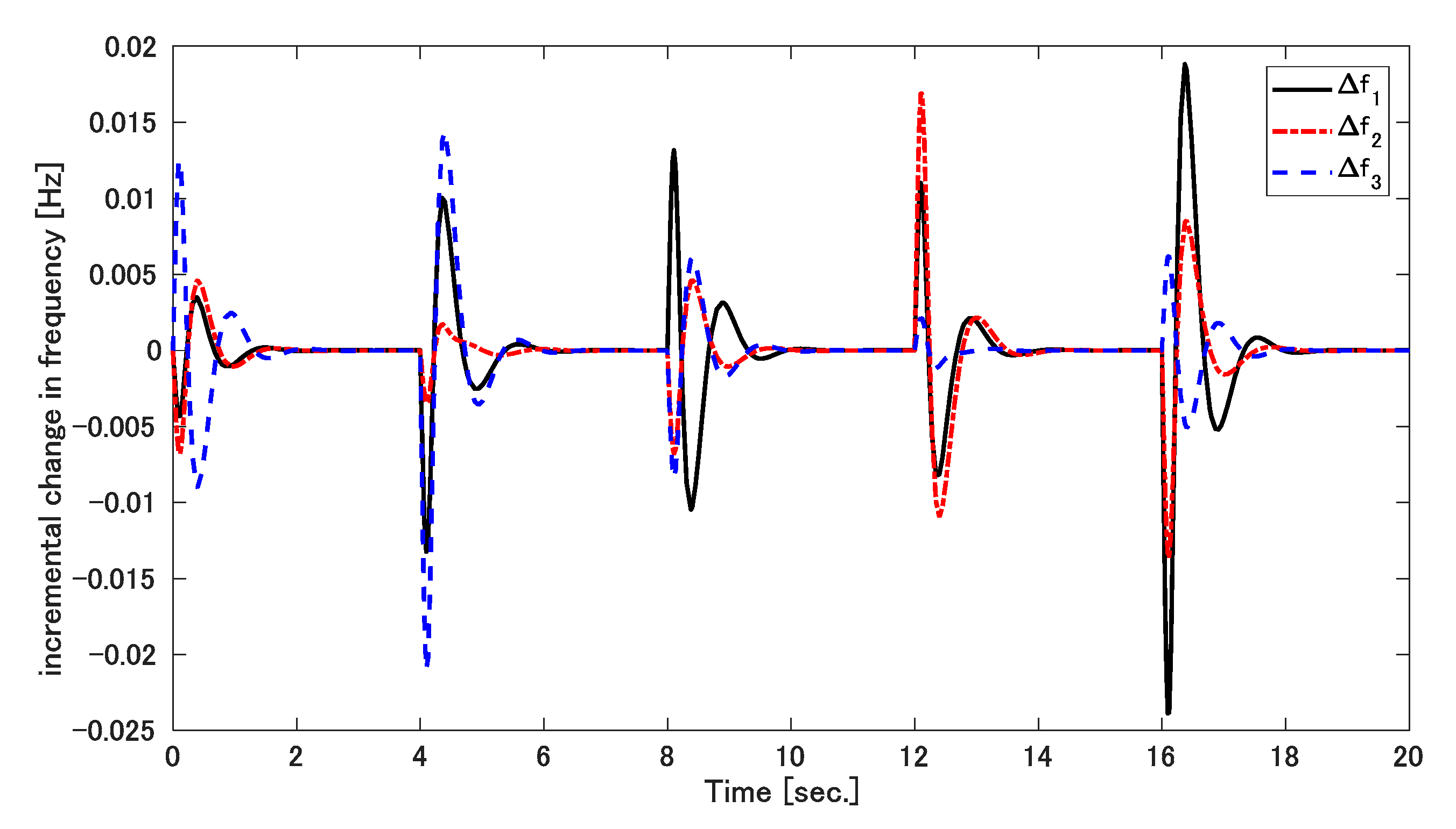
Therefore, the New England PS was simulated with and without wind plants to test the proposed continuous decentralized second-order SMC based observer. Figure 19 and Figure 20 illustrate the results of the frequency error and the tie-line power error of the New England PS without wind. With the use of system states estimated by the observer, the frequency maximum overshoot and settling time were comparatively lower than the results presented in [34]. This is evidence that the new approach has a higher damping ratio than the scheme in [34]. In addition, the proposed approach solved the chattering phenomenon inherent in the first-order SMC presented in [32]. On the other hand, Figure 21 and Figure 22 display the results of the frequency deviation and tie-power error of the New England PS with wind turbines. As seen in Figure 21 and Figure 22, the MAIPS was also stable with good performance.
Remark 4.
An SMC based on the observer used for the LFC of the New England PS can be seen in [34]. However, there are two limitations of the above approach. The first is that the system state variables need to be measured in order to provide feedback for the controller. The second is that the control suffers from the chattering problem inherent in the first-order SMC. In this approach, the state observer is used in the sliding surface and second-order sliding mode controller. Therefore, the two above limitations have been solved.

6. Conclusions

The need for the MAIPS integrated with wind plants is increasing day by day because of the need for efficient power generation. However, the wind variation problem associated with wind turbines can make MAIPS frequency unstable. Therefore, the LFC is important in order to regulate frequency and provide better power quality to consumers. In order to solve the above problem, a new LFC for an MAIPS integrated with wind plants using a state observer based on sliding mode, acting under a second-order time derivative, has been developed. The continuous decentralized sliding mode controller guarantees the control signal accuracy so that the performance of the MAIPS and the power quality are improved. In addition, the stability of the entire power network was demonstrated by means of the Lyapunov method based on the new LMI technique. The simulation results show that the frequency error and the tie-line power error rapidly converge to zero, with better settling time and overshoot when compared to existing designs. Furthermore, the proposed controller can handle with the wind variation because the results show less impact on the power system frequency and tie-line power deviation. In order to verify this new approach with a real MAIPS, a New England PS with and without a wind plant was used and the results showed an improvement in the system performance with respect to maximum overshoot and settling time. Thus, the proposed approach is a better choice for the LFC of a real MAIPS with a wind plant.

Author Contributions

Conceptualization V.V.H., E.N.A. and T.M.N.; methodology P.T.T., A.-T.T., E.N.A., and V.-T.P.; software A.-T.T. and E.N.A.; validation B.L.N.M., P.T.T. and V.-T.P.; writing—original draft preparation E.N.A., A.-T.T. and P.T.T.; writing—review and editing V.V.H., V.-T.P., T.M.N., B.L.N.M. and V.-D.P.; supervision B.L.N.M., T.M.N., V.V.H. and V.-D.P. All authors have read and agreed to the published version of the manuscript.

Funding

This research was funded by the Foundation for Science and Technology Development of Ton Duc Thang University (FOSTECT), website: http://fostect.tdtu.edu.vn, under Grant FOSTECT.2017.BR.05.

Institutional Review Board Statement

Not applicable.

Informed Consent Statement

Not applicable.

Data Availability Statement

The data presented in this study are available on reasonable request from the corresponding author.

Conflicts of Interest

The authors declare no conflict of interest.

References

  1. Hsu, K.C. Decentralized variable structure model-following adaptive control for interconnected systems with series nonlinearities. Int. J. Syst. Sci. 1998, 29, 365–372. [Google Scholar] [CrossRef]
  2. Bevrani, H.; Mitani, Y.; Tsuji, K. Robust decentralized load-frequency control using an iterative linear matrix inequalities algorithm. IEE Proc. Gener. Trans. Distrib. 2004, 151, 347–354. [Google Scholar] [CrossRef] [Green Version]
  3. Thirunavukarasu, R.; Chidambaram, I.A. PI2 controller based coordinated control with redox flow battery and unified power flow controller for improved restoration indices in a deregulated power system. Ain Shams Eng. J. 2016, 7, 1011–1102. [Google Scholar] [CrossRef]
  4. Farahani, M.; Ganjefar, S.; Alizadeh, M. PID controller adjustment using chaotic optimization algorithm for multi-area load frequency control. IET Control Theory Appl. 2012, 6, 1984–1992. [Google Scholar] [CrossRef]
  5. Saxena, S.; Hote, Y.V. Decentralized PID load frequency control for perturbed multi-area power systems. Int. J. Electr. Power Energy Syst. 2016, 81, 405–415. [Google Scholar] [CrossRef]
  6. Alrifai, M.T.; Hassan, M.F.; Zribi, M. Decentralized load frequency controller for a multi-area interconnected power system. Int. J. Electr. Power Energy Syst. 2011, 33, 198–209. [Google Scholar] [CrossRef]
  7. Zhao, C.; Topcu, U.; Low, S.H. Optimal load control via frequency measurement and neighborhood area communication. IEEE Trans. Power Syst. 2013, 28, 3576–3587. [Google Scholar] [CrossRef] [Green Version]
  8. Abdennour, A. Adaptive optimal gain scheduling for the load frequency control problem. Electr. Power Compon. Syst. 2002, 30, 45–56. [Google Scholar] [CrossRef]
  9. Daneshfar, F.; Bevrani, H. Load-frequency control: A GA based multi-agent reinforcement learning. IET Gener. Trans. Distrib. 2010, 4, 13–26. [Google Scholar] [CrossRef] [Green Version]
  10. Saxena, S.; Hote, Y.V. Load frequency control in power systems via internal model control scheme and model-order reduction. IEEE Trans. Power Syst. 2013, 28, 2749–2757. [Google Scholar] [CrossRef]
  11. Ersdal, A.M.; Imsland, L.; Uhlen, K. Model predictive load-frequency control. IEEE Trans. Power Syst. 2016, 31, 777–785. [Google Scholar] [CrossRef] [Green Version]
  12. Chang-Chien, L.R.; Wu, Y.S.; Cheng, J.S. Online estimation of system parameters for artificial intelligence applications to load frequency control. IET Gener. Trans. Distrib. 2010, 5, 895–902. [Google Scholar] [CrossRef]
  13. Yousef, H. Adaptive fuzzy logic load frequency control of multi-area power system. Int. J. Electr. Power Energy Syst. 2015, 68, 384–395. [Google Scholar] [CrossRef]
  14. Liu, F.; Li, Y.; Cao, Y.; She, J.; Wu, M. A two-layer active disturbance rejection controller design for load frequency control of interconnected power system. IEEE Trans. Power Syst. 2016, 31, 3320–3321. [Google Scholar] [CrossRef]
  15. Liu, Y.; Lan, Q.; Qian, C.; Qian, W.; Chu, H. Universal finite time observer design and adaptive frequency regulation of hydraulic turbine systems. IET Control Theory Appl. 2016, 10, 363–370. [Google Scholar] [CrossRef]
  16. Chen, H.; Sun, N. Nonlinear control of under-actuated systems subject to both actuated and unactuated state constraints with experimental verification. IEEE Trans. Ind. Electr. 2019, 67, 7702–7714. [Google Scholar] [CrossRef]
  17. Sun, Y.; Qiang, H.; Mei, X.; Teng, Y. Modified repetitive learning control with unidirectional control input for uncertain nonlinear systems. Neural Comput. Appl. 2018, 30, 2003–2012. [Google Scholar] [CrossRef]
  18. Bevrani, H. Robust Power System Frequency Control; Springer: New York, NY, USA, 2009. [Google Scholar]
  19. Mi, Y.; Fu, Y.; Wang, C.; Wang, P. Decentralized sliding mode load frequency control for multi-area power systems. IEEE Trans. Power Syst. 2013, 28, 4301–4309. [Google Scholar] [CrossRef]
  20. Onyeka, A.E.; Xing-Gang, Y.; Mao, Z.; Jiang, B.; Zhang, Q. Robust decentralized load frequency control for interconnected time delay power systems using sliding mode techniques. IET Control Theory Appl. 2019, 14, 470–480. [Google Scholar] [CrossRef] [Green Version]
  21. Guo, J. Application of a novel adaptive sliding mode control method to the load frequency control. Eur. J. Control 2020, 57, 172–178. [Google Scholar]
  22. Lv, X.; Sun, Y.; Wang, Y.; Dinavahi, V. Adaptive event-triggered load frequency control of multi-area power systems under networked environment via sliding mode control. IEEE Access 2020, 8, 86585–86594. [Google Scholar] [CrossRef]
  23. Le Ngnoc Minh, B.; Huynh, V.V.; Nguyen, T.M.; Tsai, Y.W. Decentralized adaptive double integral sliding mode controller for multi-area power systems. Math. Probl. Eng. 2018, 2018, 1–11. [Google Scholar] [CrossRef]
  24. Huynh, V.V.; Tran, P.T.; Minh, B.L.N.; Tran, A.T.; Tuan, D.H.; Nguyen, T.M.; Vu, P.T. New second-order sliding mode control design for load frequency control of a power system. Energies 2020, 13, 6509. [Google Scholar] [CrossRef]
  25. Kalla, U.K.; Singh, B.; Murthy, S.S.; Jain, C.; Kant, K. Adaptive sliding mode control of standalone single-phase microgrid using hydro, wind, and solar PV array-based generation. IEEE Trans. Smart Grid 2017, 9, 6806–6814. [Google Scholar] [CrossRef]
  26. Dev, A.; Sarkar, M.K.; Asthana, P.; Narzary, D. Event-Triggered adaptive integral higher-order sliding mode control for load frequency problems in multi-area power systems. Iran. J. Sci. Technol. Trans. Electr. Eng. 2019, 43, 137–152. [Google Scholar] [CrossRef]
  27. Sarkar, M.K.; Dev, A.; Asthana, P.; Narzary, D. Chattering free robust adaptive integral higher order sliding mode control for load frequency problems in multi-area power systems. IET Control Theory Appl. 2018, 12, 1216–1227. [Google Scholar] [CrossRef]
  28. Rosyiana, F.I.; Kim, J.S.; Song, H. High-gain disturbance observer-based robust load frequency control of power systems with multiple areas. Energies 2017, 10, 595. [Google Scholar]
  29. Mi, Y.; Fu, Y.; Li, D.; Wang, C.; Loh, P.C.; Wang, P. The sliding mode load frequency control for hybrid power system based on disturbance observer. Int. J. Electr. Power Energy Syst. 2016, 74, 446–452. [Google Scholar] [CrossRef]
  30. Wang, C.; Mi, Y.; Fu, Y.; Wang, P. Frequency control of an isolated micro-grid using double sliding mode controllers and disturbance observer. IEEE Trans. Smart Grid 2016, 9, 923–930. [Google Scholar] [CrossRef]
  31. Liao, K.; Xu, Y. A robust load frequency control scheme for power systems based on second-order sliding mode and extended disturbance observer. IEEE Trans. Ind. Inf. 2017, 14, 3076–3086. [Google Scholar] [CrossRef]
  32. Huynh, V.V.; Minh, B.L.N.; Amaefule, E.N.; Tran, A.T.; Tran, P.T. Highly robust observer sliding mode based frequency control for multi area power systems with renewable power plants. Electronics 2021, 10, 274. [Google Scholar] [CrossRef]
  33. Tummala, A.S.; Inapakurthi, R.; Ramanarao, P.V. Observer based sliding mode frequency control for multi-machine power systems with high renewable energy. J. Mod. Power Syst. Clean Energy 2018, 6, 473–474. [Google Scholar] [CrossRef] [Green Version]
  34. Prasad, S.; Purwar, S.; Kishor, N. Load frequency regulation using observer based non-linear sliding mode control. Int. J. Electr. Power Energy Syst. 2019, 104, 178–193. [Google Scholar] [CrossRef]
  35. Liu, X.; Wang, P.; Loh, P.C. A hybrid AC/DC microgrid and its coordination control. IEEE Trans. Smart Grid 2011, 2, 278–286. [Google Scholar]
  36. Obaid, Z.A.; Cipcigan, L.M.; Abrahim, L.; Muhssin, M.T. Frequency control of future power systems: Reviewing and evaluating challenges and new control methods. J. Mod. Power Syst. Clean Energy 2019, 7, 9–25. [Google Scholar] [CrossRef]
  37. Bucolo, M.; Buscarino, A.; Famoso CFortuna, L.; Frasca, M. Control of imperfect dynamical systems. Nonlinear Dyn. 2019, 98, 2989–2999. [Google Scholar] [CrossRef]
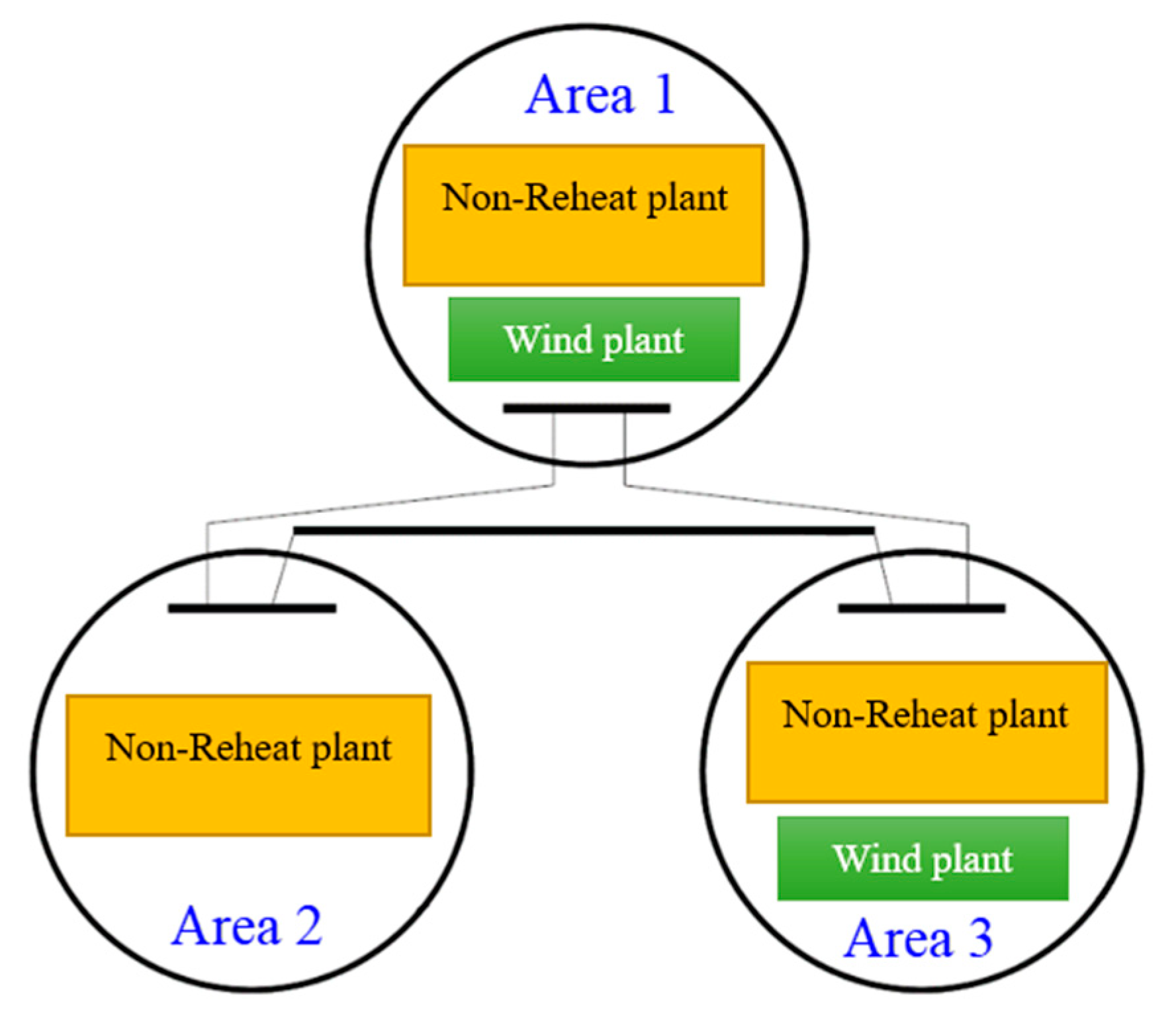
Figure 1. A simplified sketch of a three-area integrated wind plant system.
Applsci 11 03051 g001
Figure 2. Schematic block diagram sketch for ith area network, including a wind farm.
Applsci 11 03051 g002
Figure 3. Diagram of a three-area power system integrated with a wind plant.
Applsci 11 03051 g003
Figure 4. Frequency deviation of three-area power system.
Applsci 11 03051 g004
Figure 5. Tie-line power of three-area power system.
Applsci 11 03051 g005
Figure 6. Control signal of three-area power system.
Applsci 11 03051 g006
Figure 7. Wind speed variation.
Applsci 11 03051 g007
Figure 8. Frequency deviation of three-area power system without a wind plant.
Applsci 11 03051 g008
Figure 9. Frequency deviation of three-area power system with a wind plant.
Applsci 11 03051 g009
Figure 10. Tie-line power deviation of three-area power system without a wind plant.
Applsci 11 03051 g010
Figure 11. Tie-line power deviation of three-area power system with a wind plant.
Applsci 11 03051 g011
Figure 12. Frequency deviation of three-area power system without a wind plant.
Applsci 11 03051 g012
Figure 13. Frequency deviation of three-area power system with a wind plant.
Applsci 11 03051 g013
Figure 14. Tie-line power deviation of three-area power system without a wind plant.
Applsci 11 03051 g014
Figure 15. Tie-line power deviation of three-area power system with a wind plant.
Applsci 11 03051 g015
Figure 16. Diagram of IEEE 39-bus integrated with wind plant.
Applsci 11 03051 g016
Figure 17. Wind speed variation.
Applsci 11 03051 g017
Figure 18. Load variations.
Applsci 11 03051 g018
Figure 19. Frequency deviation without wind plant.
Applsci 11 03051 g019
Figure 20. Tie-line power deviation without wind plant.
Applsci 11 03051 g020
Figure 21. Frequency deviation with wind plant.
Applsci 11 03051 g021
Figure 22. Tie-line power deviation with wind plant.
Applsci 11 03051 g022
Table 1. Setting time and maximum overshoot of the proposed state observer based on sliding mode control (SOboSMC) and double-integral SMC [23].
Kind of ControllerProposed SOboSMCDouble Integral SMC
[23]
Parameters T s ( t ) Max.O. S (pu) T s ( t ) Max.O. S (pu)
Δ f 1 3 5.8 × 10 3 7 0.06
Δ f 2 3 6.5 × 10 3 7 0.07
Δ f 3 3 11.5 × 10 3 7 0.07
Publisher’s Note: MDPI stays neutral with regard to jurisdictional claims in published maps and institutional affiliations.