Wind Turbine Power Curve Modelling with Logistic Functions Based on Quantile Regression

Featured Application

The research proposed in this paper could be useful in wind power forecasting, condition monitoring and energy assessment of wind turbine.

Abstract

The wind turbine power curve (WTPC) is of great significance for wind power forecasting, condition monitoring, and energy assessment. This paper proposes a novel WTPC modelling method with logistic functions based on quantile regression (QRLF). Firstly, we combine the asymmetric absolute value function from the quantile regression (QR) cost function with logistic functions (LF), so that the proposed method can describe the uncertainty of wind power by the fitting curves of different quantiles without considering the prior distribution of wind power. Among them, three optimization algorithms are selected to make comparative studies. Secondly, an adaptive outlier filtering method is developed based on QRLF, which can eliminate the outliers by the symmetrical relationship of power distribution. Lastly, supervisory control and data acquisition (SCADA) data collected from wind turbines in three wind farms are used to evaluate the performance of the proposed method. Five evaluation metrics are applied for the comparative analysis. Compared with typical WTPC models, QRLF has better fitting performance in both deterministic and probabilistic power curve modeling.

1. Introduction

The wind turbine power curve (WTPC) is defined as the relationship between electrical power output and hub height wind speed of a wind turbine [1], and it is important for energy assessment, wind power forecasting and condition monitoring [2]. As mentioned in [3], the manufacturer provides a design power curve to describe the characteristics of wind turbine power generation. However, affected by the variability of the local environment and the adjustment of wind turbine internal parameters, the design power curve is unable to meet the requirements of wind farm operators. To enhance the fitting accuracy, many published literatures used supervisory control and data acquisition (SCADA) data to establish data-driven WTPC models, which are generally divided into parametric methods and nonparametric methods [4].

Parametric methods are based on solving mathematical expressions, including determination of expressions and parameter estimation. According to [5], linearized segmented model has been widely used in practical production. In [4,6], polynomial regression (PR) with different orders was used for WTPC modelling, and the results show that 6th-order and 9th-order PR have better fitting accuracy. In addition to PR, exponential functions, hyperbolic tangent functions and power coefficient methods have all been applied for WTPC modelling [7,8]. In recent years, logistic functions (LF) have been utilized for WTPC fitting because of their continuity and good nonlinear mapping ability [9,10,11,12]. Reference [9] made comparative studies of LF with three to six model parameters, and the results show that 5-parameter logistic function (5PL) generally has the best fitting effect.

Nonparametric methods do not impose any prespecified mathematical expressions, and the modelling process is entirely based on the observed data. Reference [13] proved that cubic spline interpolation (CSI) can fit smooth and accurate power curves. Reference [14] divided the raw dataset into 10 phases according to K-means clustering, and for each phase, smoothing spline was utilized as the fitting function. With the development of statistics and computer science, machine learning techniques such as neural networks (NN) [15], adaptive neural-fuzzy inference systems (ANIFS) [16] and K-Nearest Neighbors (KNN) [17] have been gradually applied for WTPC modelling.

Most of the aforementioned methods belong to deterministic WTPC models, which only describe the relationship between wind speed and power average but cannot reflect the uncertainty of wind power. Accordingly, probabilistic WTPC models were developed to reveal the variation and uncertainty of the power generation process, and improve the reliability for WTPC based applications, such as energy assessment and condition monitoring [18]. According to [19,20,21,22,23], the Gaussian process (GP) is the widely used method for probabilistic WTPC modelling, which can qualify the uncertainty of power generation via the predicted confidence intervals (CI). To reduce the computation cost, [20] used Cholesky decomposition to solve the inverse matrix in GP. Reference [21] proposed a heteroscedastic GP to enhance the interval predictions. Reference [22] combined GP with LF and proposed a semi-parametric model for probabilistic WTPC modelling. Reference [23] indicated that adding pitch angle and rotor to the model inputs of GP can improve the fitting accuracy. In [24], a multivariate WTPC was established by using support vector machine (SVM) with Gaussian kernel. Reference [25] combined SVM with pointwise CI and simultaneous CI to estimate the uncertainty of wind power. The Monte Carlo algorithm [18], Copula function [26] and relevance vector machine (RVM) [27] were also applied for probabilistic WTPC modelling.

The key challenges of most probabilistic WTPC models lies in the assumption that the wind power follows a specific prior distribution during the training process. In practical conditions, however, the distribution of wind power at different times or conditions is inconsistent [18], and this problem will decrease the accuracy of the predicted CI. Reference [28] established a probabilistic WTPC by moving the power curves fitted by B-Spline. Although it does not need to assume a prior distribution, only power average information is used during the modelling process. Quantile regression (QR) provides an effective regression analysis method without considering the distribution pattern of random variables [29]. Reference [30] used a multi-core parallel quantile regression neural network (QRNN) for probabilistic wind power forecasting. However, there are few QR based WTPC models in recent published literatures. In addition, power outliers will decrease the fitting accuracy of WTPC. Reference [15] filtered the power outliers by setting thresholds based on GP, but it cannot effectively eliminate the stacked outliers caused by wind curtailment. According to [31,32], stacked outliers can be filtered by clustering algorithms, such as fuzzy c-means and DBSCAN. In some cases, however, these methods lead to a high proportion of normal data being eliminated.

This paper proposes a novel WTPC modelling method with logistic functions based on quantile regression (QRLF). The major contributions are summarized as follows. (1) Typical LF based methods have good performance in WTPC modelling, but only deterministic fitting results can be obtained. Considering the structure of LF and QR, we combine the asymmetric absolute value function from the QR cost function [29] with the LF model parameters, so that the proposed method can describe the uncertainty of wind power by the fitting curves of different quantiles. (2) When the wind turbine is operating normally, the distribution of power at a given wind speed is approximately symmetric about the mean [33]. According to that, we propose a novel outlier filtering method that utilizes the symmetrical relationship of power distribution. It can effectively filter both sparse outliers and stacked outliers, and adjust the number of iterations according to the number of power outliers. To further evaluate the performance of the proposed method, both deterministic and probabilistic evaluation metrics are applied to evaluate the performance of the proposed WTPC model. The results show that the QRLF based power curve model is able to provide both accurate deterministic fitting results and an appropriate predicted CI.

The rest of this paper is organized as follows. Section 2 presents the mathematical principle of QRLF. Section 3 introduces the WTPC modelling process based on QRLF. The case study is shown in Section 4. Conclusions are drawn in Section 5.

2. The Proposed Logistic Functions Based on Quantile Regression

2.1. Logistic Functions

Logistic functions (LF) have been successfully applied in WTPC modelling due to their good nonlinear mapping ability. Among them, 4-parameter logistic function (4PL) has been commonly used, expressed as [9]:

$$P(v,\mathsf{\theta })=a\cdot \frac{1+m\cdot \exp (v/\tau )}{1+n\cdot \exp (v/\tau )}$$

(1)

where P(v, θ) is the predicted power output; v is the wind speed; and θ = [a, m, n, τ]. We can obtain the estimated parameters $\widehat{\mathsf{\theta }}$ of 4PL by minimizing the following cost function:

$$\widehat{\mathsf{\theta }}=\arg \min {\displaystyle \sum _{i=1}^N{[y_i-P(v_i,\mathsf{\theta })]}^2}$$

(2)

where N is the number of samples in training set and y_i is the observed power output.

Fitting curves obtained by 4PL, however, are point symmetric on the semi-log axis about its midpoint, which cannot accurately fit the power curves with asymmetric features [34]. Accordingly, researchers proposed a 5-parameter logistic function (5PL) to enhance the mapping ability for asymmetric data, expressed as:

$$P(v,\mathsf{\theta })=d+\frac{a-d}{{(1+{(v/c)}^b)}^g}$$

(3)

where, in 5PL, θ = [a, b, c, d, g], c, g > 0; parameters a and d determine the position of the horizontal asymptote of the fitting curve; and g is the asymmetry factor. The curvature of the fitting curve is jointly controlled via b, c and g. Although 5PL has good nonlinear mapping ability in power curve modelling, it can only provide deterministic fitting results.

2.2. Quantile Regression

Quantile regression (QR) provides an effective method for estimating models for conditional quantile functions [29]. Therefore, the uncertainty of wind power can be described by using the fitting curves of different conditional quantiles without imposing stringent parametric assumptions. Generally, QR can be regarded as an extension of a linear model, expressed as:

$$P(v,\mathsf{\beta }(\tau ))={\beta }_0(\tau )+{\beta }_1(\tau )v+{\beta }_0(\tau )v^2+\dots +{\beta }_n(\tau )v^k$$

(4)

where P(v, β(τ)) is the predicted power output at τth conditional quantile and β(τ) = [β₀(τ), β₁(τ),…, β_n(τ)] is the model parameter vector in τ-quantile, obtained by:

$$\hat{\mathsf{\beta }}(\tau )=\arg \min {\displaystyle \sum _{i=1}^N{\rho }_{\tau }[y_i-P(v_i,\mathsf{\beta }(\tau ))]}$$

(5)

$${\rho }_{\tau }(u)=\{\begin{array}{cc}\tau u,\hfill & u\ge 0\hfill \\ (1-\tau )u,\hfill & u<0\hfill \end{array}\tau \in (0,1)$$

(6)

where ρ_τ(u) is the asymmetric absolute value function [29]. However, QR based methods have limitations in complex nonlinear curve fitting. Previous studies attempted to combine QR with a neural network and support vector machine to enhance its nonlinear mapping ability [35], but the fitting accuracy of the predicted CI was still unable to meet the requirements of wind farms.

2.3. Logistic Functions Based Quantile Regression

In this paper, we combine the asymmetric absolute value function from the QR cost function with 5PL, and propose a novel probabilistic logistic function for WTPC modelling. The expression is given by:

$$P(v,\mathsf{\theta }(\tau ))=d(\tau )+\frac{a(\tau )-d(\tau )}{{(1+{(v(\tau )/c(\tau ))}^{b(\tau )})}^{g(\tau )}}$$

(7)

where θ(τ) = [a(τ), b(τ), c(τ), d(τ), g(τ)] is the model parameter vector in τ-quantile, which can be estimated by minimizing the cost function:

$$\widehat{\mathsf{\theta }}(\tau )=\arg \min {\displaystyle \sum _{i=1}^N{\rho }_{\tau }[y_i-P(v_i,\mathsf{\theta }(\tau ))]}$$

(8)

Adding ρ_τ(.) to the cost function of QRLF increases the complexity of parameter optimization. In order to obtain the optimal estimation of $\widehat{\mathsf{\theta }}$, two meta-heuristic optimization algorithms and a gradient based optimization algorithm are utilized in this paper for comparative studies.

2.4. Parameter Optimization Algorithms

Particle swarm optimization (PSO) has been successfully applied in deterministic power curve modelling (including LF with different model parameters) [8]. Considering the similarity between logistic functions and the proposed QRLF, this paper selects PSO as one of the optimization algorithms. According to [36], the whale optimization algorithm (WOA) is a meta-heuristic algorithm that can be utilized for optimizing complex nonlinear problems. During the optimization process, a spiral equation is added to enhance the robustness and prevent the results from falling into the local optimum. In addition, we attempt to use different types of gradient based algorithms to optimize the model parameters. Among them, the Adam optimization algorithm is selected to make comparative studies with PSO and WOA.

2.4.1. Particle Swarm Optimization

Particle swarm optimization (PSO) solves optimization problems by defining and moving particles around in the search-space over the particle’s position and velocity [37]. Reference [38] added the inertia weight parameter to improve the performance of PSO, and the expressions are as follows:

$$\begin{array}{l}{v}_i(t+1)=\omega \cdot v_i(t)+c_1\cdot rand(0,1)\cdot (p_i(t)-x_i(t))+c_2\cdot rand(0,1)\cdot (g(t)-x_i(t))\\ x_i(t+1)=x_i(t)+v_i(t+1)\end{array}$$

(9)

where v_i and x_i are the velocity and position vectors of particle i; p_i is the best position vector of particle i; g is the best position vector of the entire swarm; ω is the inertia weight, c₁ and c₂ are acceleration constants; and t is the number of iterations. After numerous iterations, we can get the global optimal solution of the estimated model parameters.

2.4.2. Whale Optimization Algorithm

The whale optimization algorithm (WOA) is inspired by the social behavior of humpback whales, which consists of the search for prey, encircling prey and bubble-net foraging mechanisms [36]. The mathematical expressions are as follows:

$$w_i(t+1)=\{\begin{array}{cc}\left|w*(t)-w_i(t)\right|\cdot e^l\cdot \cos (2\pi l)+w*(t),\hfill & \hfill p\ge 0.5\\ w*(t)-A\cdot \left|2r\cdot w*(t)-w_i(t)\right|,\hfill & \hfill p<0.5\&\left|A\right|\le 1\\ w_{rand}-A\cdot \left|2r\cdot w_{rand}(t)-w_i(t)\right|,\hfill & \hfill p<0.5\&\left|A\right|>1\end{array}$$

(10)

here w_i is the position vector of search agent i; w_rand is the position vector of a random selected search agent; w* is the best position vector; r is a random vector in [0, 1]; l and p are random numbers in [0, 1] and [−1, 1]; and A is the coefficient vector, calculated by:

$$A=(4r-2)\cdot \frac{(t_{\max }-t)}{t_{\max }}$$

(11)

where t_max is the maximum number of iterations. If |A| ≤ 1, w_i is updated by w* (search for prey), but if |A| > 1, w_i is updated by w_rand (encircling prey). With the increase in iterations, the maximum value of |A| gradually decreases from 2 to 0. On the other hand, WOA randomly switches the movement mode of search agents so as to mimic the behavior of humpback whales, e.g., if p ≥ 0.5, the position of search agents will be spiral updated (bubble-net foraging).

2.4.3. Adam Optimization Algorithm

The Adam optimization algorithm combines the advantages of AdaGrad and RMSProp, and has been proven to have the ability to solve nonconvex optimization problems in the field of deep learning [39]. The expressions are as follows:

$$\begin{array}{l}{m}_t={\gamma }_1\cdot m_{t-1}+(1-{\gamma }_1)\cdot {\nabla }_{\mathsf{\theta }}f({\mathsf{\theta }}_{t-1})\\ u_t={\gamma }_2\cdot u_{t-1}+(1-{\gamma }_2)\cdot {\nabla }_{\mathsf{\theta }}^{2}f({\mathsf{\theta }}_{t-1})\end{array}$$

(12)

where θ is the parameter vector to be estimated; f(.) is the objective function; γ₁, γ₂ are exponential decay rates; t is the number of iterations; m is the first-order moment vector, m₀ = 0; and u is the second-order moment vector, u₀ = 0. After initialization, θ can be updated by:

$${\mathsf{\theta }}_t={\mathsf{\theta }}_{t-1}-\eta \cdot {\widehat{m}}_t/(\sqrt{{\widehat{u}}_t}+\epsilon )$$

(13)

where η is the learning rate; ε ≈ 0; $\widehat{m}$ and $\widehat{u}$ are moment vectors after bias correction. The detailed information of bias correction is introduced in [39].

When solving nonconvex optimization problems, falling into the local minimum is a common problem in both meta-heuristic methods and gradient based methods. Therefore, this paper repeats PSO, WOA and Adam five times, respectively, and then selects the one with the lowest fitting error to improve the stability of the aforementioned optimization algorithms.

3. WTPC Modelling with the Proposed QRLF

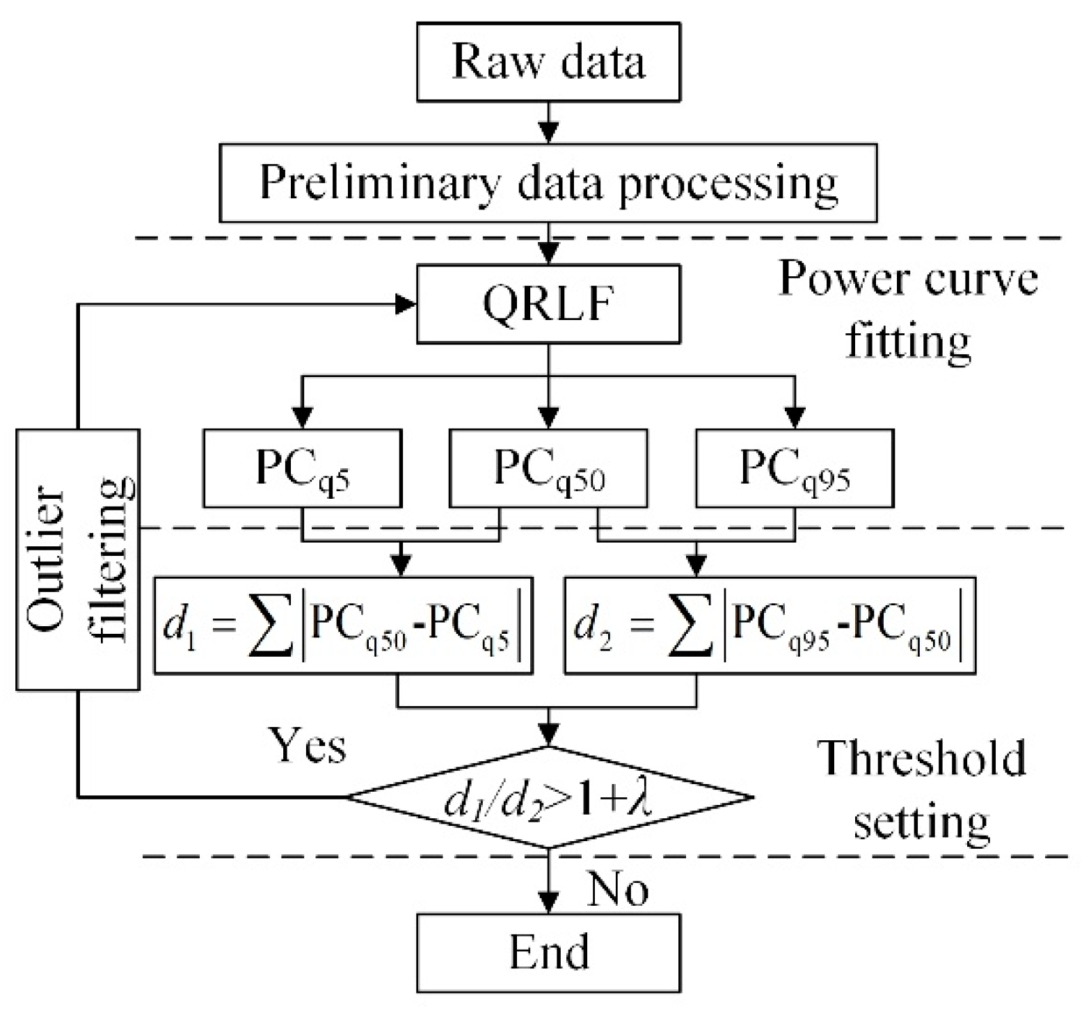
3.1. Outlier Filtering

Affected by a harsh environment and various restrictive factors, power outliers are inevitable in the collected dataset. According to [32], power outliers can be divided into sparse outliers and stacked outliers, as shown in Figure 1.

In Figure 1, sparse outliers are usually caused by random noise or a transition period where the turbine is going from shutdown to startup. Stacked outliers are mainly caused by wind curtailment, shutdown or data transmission failure (such as anemometer data error). In this paper, an outlier filtering method is proposed based on QRLF, and Figure 2 shows the flow chart.

In Figure 2, PC_q5, PC_q50, and PC_q95 are power curves fitted by QRLF (expressed in Equation (7)) with 5%, 50% and 95% quantiles, and PSO is applied for parameter optimization; λ is the hyperparameter of the proposed data filter method; d₁ is the sum of distance between PC_q5 and PC_q50; and d₂ is the distance between PC_q50 and PC_q95. The proposed outlier filtering method mainly consists of preliminary data processing, power curve fitting, threshold setting and outliers filtering.

• Preliminary data processing

Firstly, we use the state parameters to filter the stacked outliers caused by shutdown or other abnormal operation states, and then limit the value ranges of the collected data by using the design parameters of target wind turbines.

Table 1. Filtering conditions of preliminary data processing.

Parameter Name	Value	Attribute
Operation mode	32 (Normal)	State parameters
Power generation	[0.01Prated, 1.05Prated]	Operation parameters
Wind speed	[vcut-in, vcut-out]
Rotor speed	[6 r/min, 12 r/min]
Pitch angle	[0°, 20°]

lists the detailed information of the filtering conditions.

Secondly, we calculate the power coefficient (C_P) of each power point, and then filter the power points that exceed the Betz limit (16/27) [1], expressed as:

$$C_P=2P/{\rho }_{0}A{v}^3$$

(14)

where P is the power output; v is the wind speed; A is the swept area of the impeller; and ρ₀ = 1.225 is the reference air density. This step can eliminate the outliers that have higher power output than normal power points, e.g., data transmission failure in Figure 1. However, limited by the types of monitored parameters, only several kinds of outliers can be eliminated by preliminary data processing.

2.

Power curve fitting

After data preprocessing, this paper uses QRLF (optimized by PSO) with 5%, 50% and 95% quantiles to build three power curves, and then eliminates the remaining outliers by the positional relationship of these fitting curves.

3.

Threshold setting

We calculate the distance between different fitting curves (d₁ and d₂ in Figure 2), and then use the ratio of them (d₁/d₂) to quantify the relationship of relative position between fitting curves. For example, in Figure 3a, when the wind turbine is operating normally, the distribution of power at a given wind speed is approximately symmetric about the mean, d₁/d₂ = 1.14. In Figure 3b, the stacked outliers increase the distance between PC_q5 and PC_q50 but the distance between PC_q95 and PC_q50 is basically unchanged because the outliers that has higher power output than the normal power points have been eliminated in preliminary data processing. In this case, d₁/d₂ = 5.90, which is much larger than 1 (ideal case). Therefore, we can determine whether there are outliers in the raw data by setting a specific threshold based on d₁/d₂. If d₁/d₂ > 1 + λ, the outlier filtering process will be executed. Hyperparameter λ as a margin added on the ideal case, which determines the end condition of the filtering process. If λ is too large, it is difficult to eliminate the power outliers, but if λ is too small, some normal data points will be regarded as the outliers. In this study, λ is set to 0.3 by the cross validation of multiple wind turbines. In some cases, however, λ needs to be fine-tuned according to the actual condition before deployment.

4.

Outlier filtering

On the basis of step 3, when d₁/d₂ > 1 + λ, we eliminate the power points lower than PC_q5 and then repeat step 2 to step 4, until d₁/d₂ ≤ 1 + λ. Figure 4 shows the intermediate results of the iterative process, and the final results of outlier filtering. The relationship between d₁/d₂ and the number of iterations is shown in Figure 5.

In Figure 4, during the iteration, PC_q5 gradually approaches to PC_q95, but the position of PC_q95 is basically unchanged. After seven iterations, d₁/d₂ is below the threshold. At this time, most outliers are filtered while normal power points are effectively preserved. In Figure 5, the iteration process stops automatically when d₁/d₂ is lower than the threshold. It can be inferred that the proposed method has a certain adaptive processing capability, which can determine the number of iterations via the number of outliers.

3.2. WTPC Modelling with the Proposed QRLF

After outlier filtering, we determine the width of CI by setting the confidence level α. Once α is confirmed, we can get the upper and lower boundaries of CI by using QRLF with quantiles 1/2 ± α/2. If α = 0, a deterministic power curve can be obtained, i.e., the width of CI is equal to zero. At last, the probabilistic WTPC model is established by combining the confidence intervals of different quantiles.

4. Case Study

4.1. Data Sources

In this paper, SCADA data collected from three wind farms are applied to evaluate the performance of the proposed method. Among them, all wind turbines are horizontal axis wind turbine equipped with an active yaw system and electrical variable-pitch blades. Wind farm 1 (WF1) and wind farm 2 (WF2) are on-shore wind farms located in Hunan province, China (25°07′ N, 111°32′ E) and Yunnan province, China (25°42′ N, 104°17′ E). SCADA data in WF1 are collected from 01/01/2017 to 03/31/2017, and SCADA data in WF2 are collected from 03/01/2018 to 05/31/2018. Unlike WF1 and WF2, wind farm 3 (WF3) is an off-shore wind farm built in Jiangsu province, China (32°31′ N, 121°11′ E), and the data acquisition time is from 07/01/2018 to 09/30/2018. All raw data are recorded at 1Hz, and a 10 min average is used in this paper according to [4].

Table 2. Detailed information of wind turbines in each wind farm.

Attributes	WF1	WF2	WF3
Hub height	80 m	84 m	90 m
Rotor diameter	108 m	111 m	171 m
Rated power	2 MW	2 MW	5 MW
Rated wind speed	9.5 m/s	12 m/s	10.9 m/s
Cut-in wind speed	3 m/s	3 m/s	3 m/s

lists the detailed information of each wind farms. The first 70% of the measured data are used for training, and the remaining data are used for testing.

4.2. Evaluation Metrics

4.2.1. Deterministic Evaluation Metrics

Mean absolute percentage error (MAPE) and root mean square error (RMSE) are the most commonly used indicators for point prediction [8]. In order to make a better comparison of power curves between wind turbines with different installed capacity, this paper uses normalized root mean square error (NRMSE) instead of RMSE, and the mathematical expressions are as follows:

$$MAPE=\frac{1}{N}{\displaystyle {\sum }_{i=1}^N\left|\frac{P_{mea}(i)-P_{pre}(i)}{P_{mea}(i)}\right|}$$

(15)

$$NRMSE=\frac{1}{P_{rated}}\sqrt{\frac{1}{N}{\displaystyle {\sum }_{i=1}^N[P_{pre}(i)-P_{mea}(i)}{]}^2}$$

(16)

where N is size of test set; P_pre is the predicted power output; P_mea is the measured power output; and C is the installed capacity of wind turbine.

4.2.2. Probabilistic Evaluation Metrics

Prediction interval coverage probability (PICP) and prediction interval normalized average width (PINAW) are significant indicators to evaluate the performance of interval predictions, which have been successfully applied to probabilistic wind power forecasting and electrical load forecasting [30,40]. The expressions are as follows:

$$PIC{P}_{\alpha }=\frac{1}{N}{\displaystyle \sum _{i=1}^N\delta (y_i),}\delta (y_i)=\{\begin{array}{c}1,y_i\in [L_i,U_i]\\ 0,y_i\notin [L_i,U_i]\end{array}$$

(17)

$$PINA{W}_{\alpha }=\frac{1}{N}{\displaystyle \sum _{i=1}^N\frac{U_i-L_i}{y_i}}$$

(18)

where PICP_α and PINAW_α are PICP and PINAW at confidence level α; N is the size of test datasets; y_i is the observed power output; and L_i and U_i are the lower and upper boundaries of the ith predicted CI. According to [40,41], a good CI prediction should have both high PICP and low PINAW. Therefore, we use the ratio of PICP_α and PINAW_α for relative comparisons with several state-of-art probabilistic WTPC methods, expressed as:

$$N{C}_{\alpha }=PINA{W}_{\alpha }/PIC{P}_{\alpha }$$

(19)

Although there is no specific index to evaluate the fitting effect, according to [41], the smaller the NC_α, the more appropriate the predicted CI.

4.3. Experimental Results

This part first makes a comparative analysis of QRLF with different model parameters and optimization algorithms to determine the optimal model structure. Then, the measured data with power outliers are applied to verify the effectiveness of the outlier filtering method introduced in Section 3.1. Lastly we compare the QRLF based WTPC model with 5PL, RVM and QRNN to further evaluate the model performance.

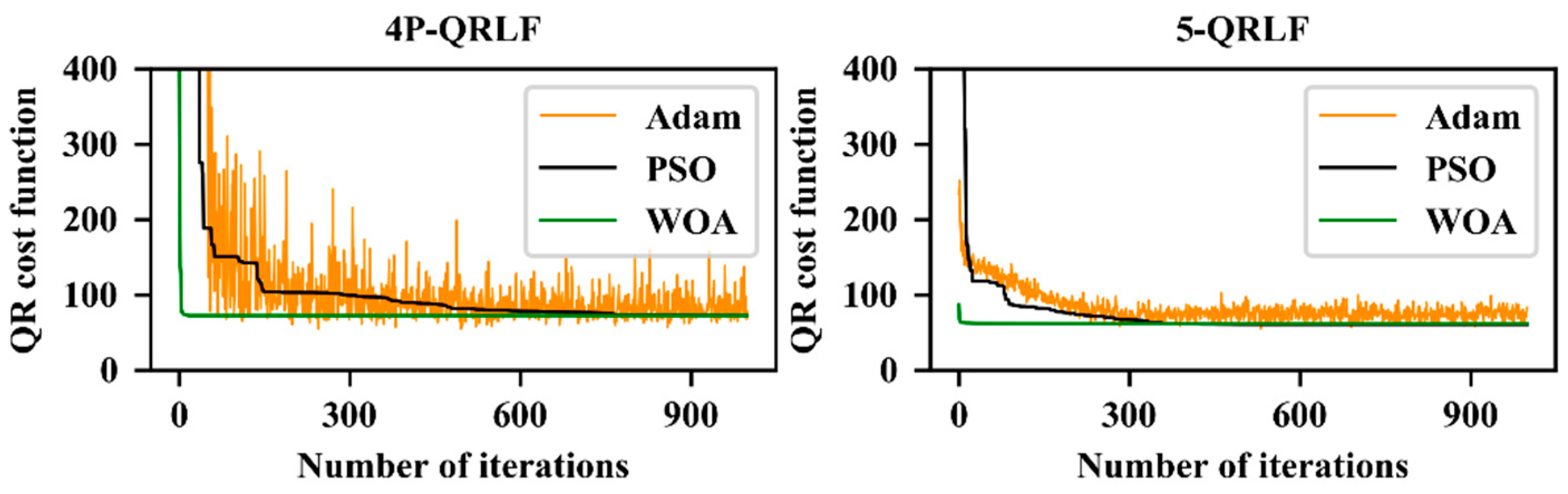
4.3.1. Results for Parameter Selection and Optimization

Before power curve fitting, we eliminate the outliers by using the method introduced in Section 3.1 to reduce the interference of power outliers on model structure determination. Then, the fitting results of three selected wind turbines in WF3 are listed in

Table 3. Fitting results of different model parameters and optimization algorithms.

Fitting Method	Optimization Algorithm	WT02			WT08			WT10
		MAPE	NRMSE	NC90%	MAPE	NRMSE	NCα	MAPE	NRMSE	NC90%
4P-QRLF	PSO	18.89%	2.04%	0.53	9.12%	1.77%	0.51	10.30%	1.94%	0.44
	WOA	19.10%	1.98%	0.62	9.31%	1.81%	0.47	9.90%	1.49%	0.46
	Adam	38.50%	2.40%	0.72	22.25%	2.37%	0.49	20.99%	2.33%	0.57
5P-QRLF	PSO	12.57%	1.52%	0.44	7.42%	1.49%	0.39	7.00%	1.37%	0.38
	WOA	9.92%	1.92%	0.57	7.31%	1.61%	0.43	8.23%	1.56%	0.41
	Adam	27.85%	1.96%	0.77	9.09%	1.81%	0.45	12.44%	1.86%	0.51

.

In Table 3, NC_90% is NC_α at the confidence level of 0.9; 4P-QRLF and 5P-QRLF are QRLF with four (five) model parameters; we can get the deterministic fitting curves when α is set to 0.5. For each type of QRLF based method, PSO, WOA and Adam optimization algorithm are used to estimate the model parameters, respectively. As mentioned in Section 2.4.3, we repeat each optimization algorithm five times to reduce the fitting error caused by local minimum.

Table 4. Control parameters of the optimization algorithms.

Algorithm	Control Parameters
PSO	particle number = 20; inertia weight (ω) = 0.8; acceleration constants (c1, c2) = 2
WOA	search agent number (whales papulation) = 40
Adam	exponential decay rates (γ1, γ2) = 0.9; learning rate = 0.0002

lists the detailed information of the control parameter for optimization algorithms, and Figure 6 shows the values of QR cost function (expressed in Equation (8)) of WT02 during the training process.

The model with the lowest fitting error is indicated by bold numbers.

As shown in Figure 6, WOA has the fastest convergence speed in both 4P-QRLF and 5P-QRLF, followed by PSO. However, Adam algorithm is difficult to converge, especially in the optimization process of 4P-QRLF. After 1000 iterations, the values of QR cost function of 4P-QRLF optimized by PSO, WOA and Adam are 72.6, 72.7 and 98.3, and the values of 5P-QRLF are 60.6, 62.2 and 83. Although the test results might be inconsistent in the repeated experiments, they generally have the same trend.

We can draw the following conclusions from the results in Table 3 and Figure 6. (1) Similar to the conclusions of previous studies on 4PL and 5PL [11], 5P-QRLF can reduce the lack-of-fit error of 4P-QRLF in asymmetry curve fitting. The results show that 5P-QRLF has better performance in both deterministic and probabilistic WTPC modelling. (2) WTPC optimized by PSO and WOA has higher fitting accuracy than Adam algorithm. The main reason is that Adam is difficult to converge during the optimization process. (3) Although the convergence speed of PSO is lower than that of WOA, it has the lowest fitting error among the above three optimization algorithms, especially in probabilistic WTPC modelling (listed in Table 3). In addition, similar conclusions can be obtained when the confidence level α is set to other values, such as 0.95 or 0.85.

According to the experimental results, this paper determines 5P-QRLF optimized by PSO as the optimal model structure of the proposed QRLF.

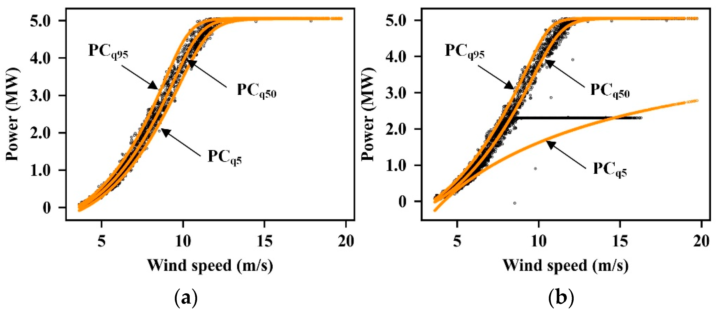
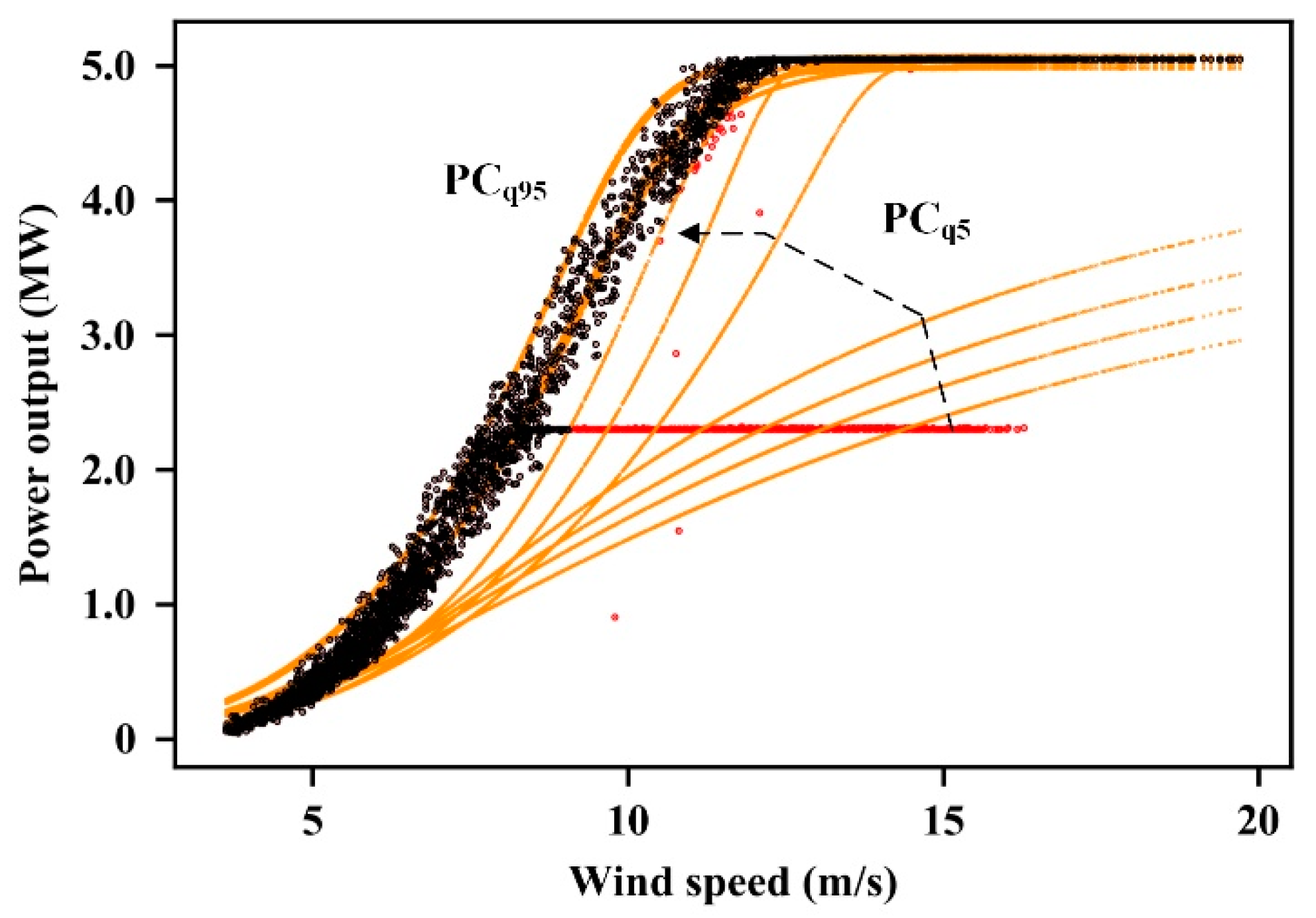
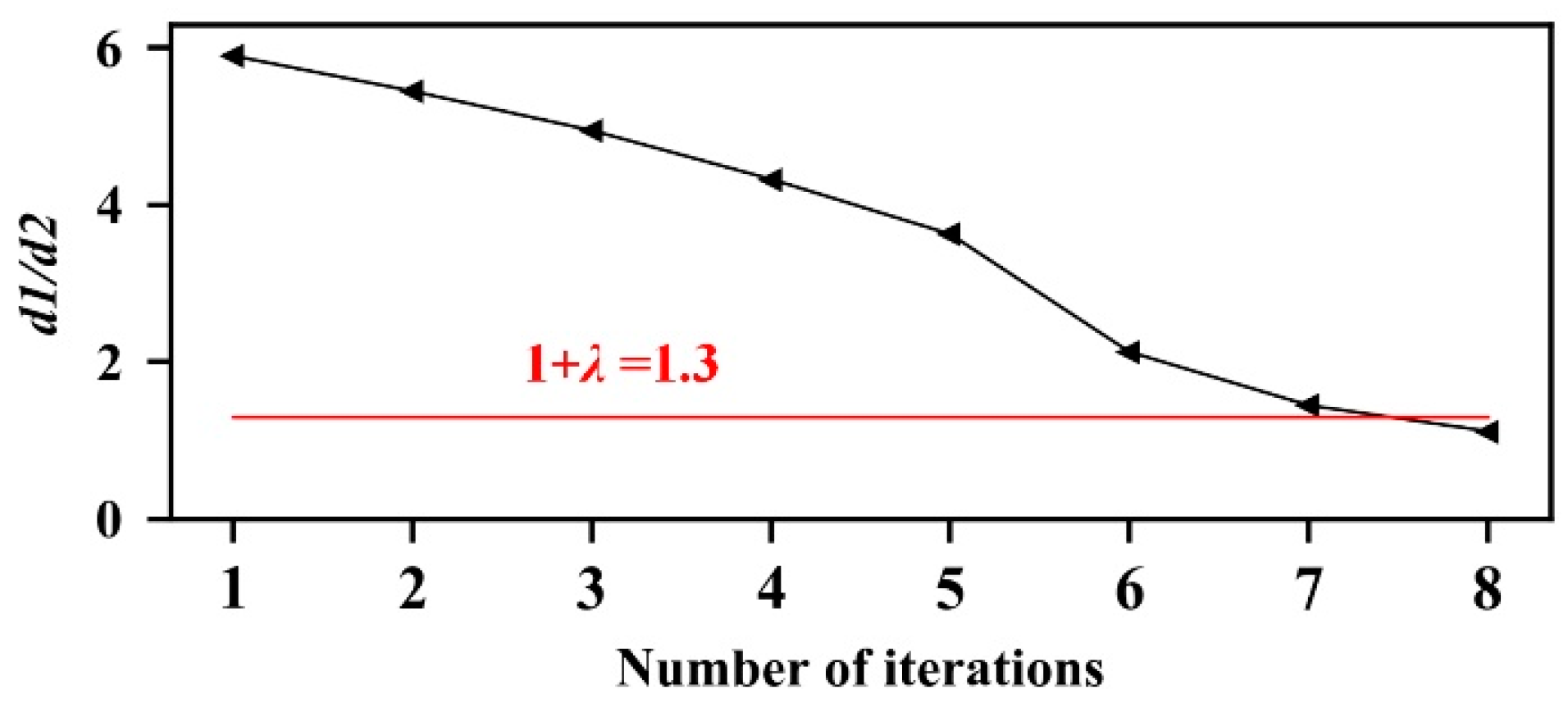
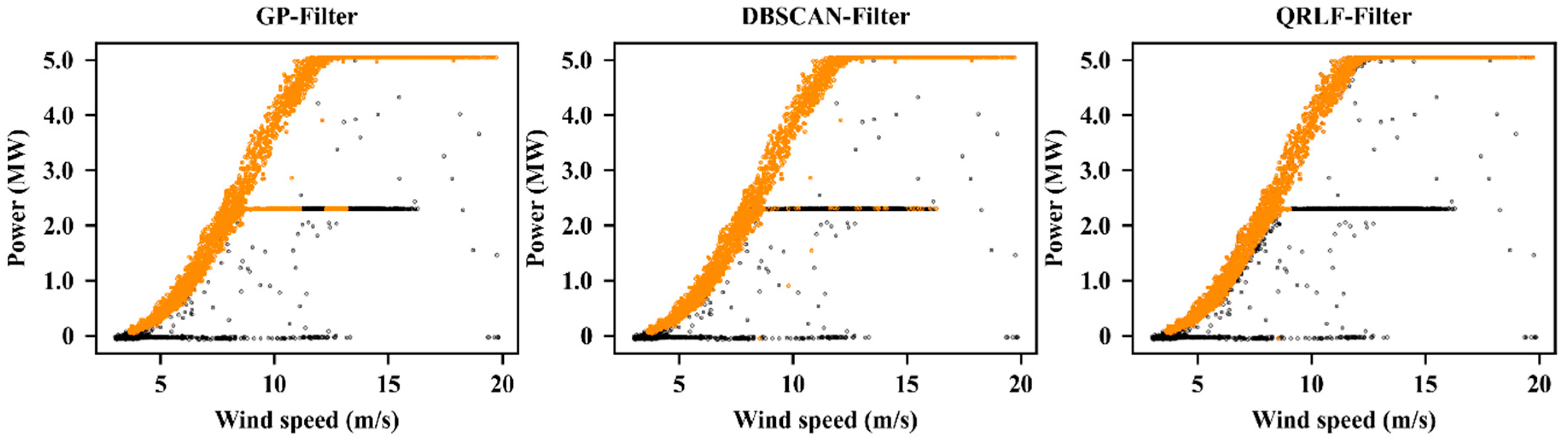
4.3.2. Results for Outlier Filtering

Similar to Section 4.3.1, three wind turbines in WF3 are selected to verify the effectiveness of the outlier filtering method based on QRLF. The scatter plots of wind speed and power output before and after outlier filtering are shown in Figure 7.

Before outlier filtering, we can clearly observe the stacked outliers caused by wind curtailment from WT08 and WT10, and few sparse outliers in the scatter plot of WT02. After outlier filtering, both sparse and stacked outliers are eliminated, while most normal data points are reserved. Among them, outliers caused by zero power output are filtered by using the monitoring parameters of the SCADA system (the first step of the proposed outlier filtering method), and then the remaining outliers are eliminated via the iterative calculations based on 5P-QRLF (step 2 to step 4). The proposed method has a certain adaptive processing capability, which can determine the number of iterations according to the number of outliers. As shown in Figure 7, after seven iterations, the outlier filtering algorithm of WT08 reaches the end condition, but for WT02, only one iteration is needed. This feature can significantly reduce the computing cost, e.g., under the same conditions, the computing time of WT08 is 181.7 s; this is more than seven times of that of WT02, i.e., 23.8 s.

For in-depth analysis, both GP based and DBSCAN based outlier filtering methods are selected to make comparative studies with the proposed method. The former one filters the outliers through removing the measurements that deviate from the expected value by more than a certain σ-dependent threshold [15], and the latter one eliminates the outliers by clustering [32]. Before filtering, we first use the same data preprocessing method (listed in Table 1) for all filtering methods to be tested to reduce the interference of other factors. Then, the model parameters are fine-tuned through cross validation in order to achieve the best filtering effect. Figure 8 shows the filtering results of one of the test wind turbines under wind curtailment.

In Figure 8, the threshold of GP based filtering method (GP-Filter) is set to 3σ; the eps and the sample numbers [32] of DBSCAN based filtering method (DBSCAN-Filter) are set to 1.2 and 20, respectively. The results show that GP-Filter is not able to effectively eliminate the stacked outliers caused by wind curtailment. Although DBSCAN-Filter can filter the abnormal power points, the filtering results are sensitive to the setting of model parameters, and it is difficult to be deployed in actual wind farm, e.g., we should fine tune the eps and sample numbers for each wind turbine (even for the same wind turbine in different time periods) to obtain the correct filtering results. Compared with DBSCAN, the proposed QRLF-Filter only has one hyperparameter λ that needs to be adjusted. The filtering results of QRLF-Filter are more robust than that of DBSCAN. Once λ is determined, we can use the same value of λ in the whole wind farm.

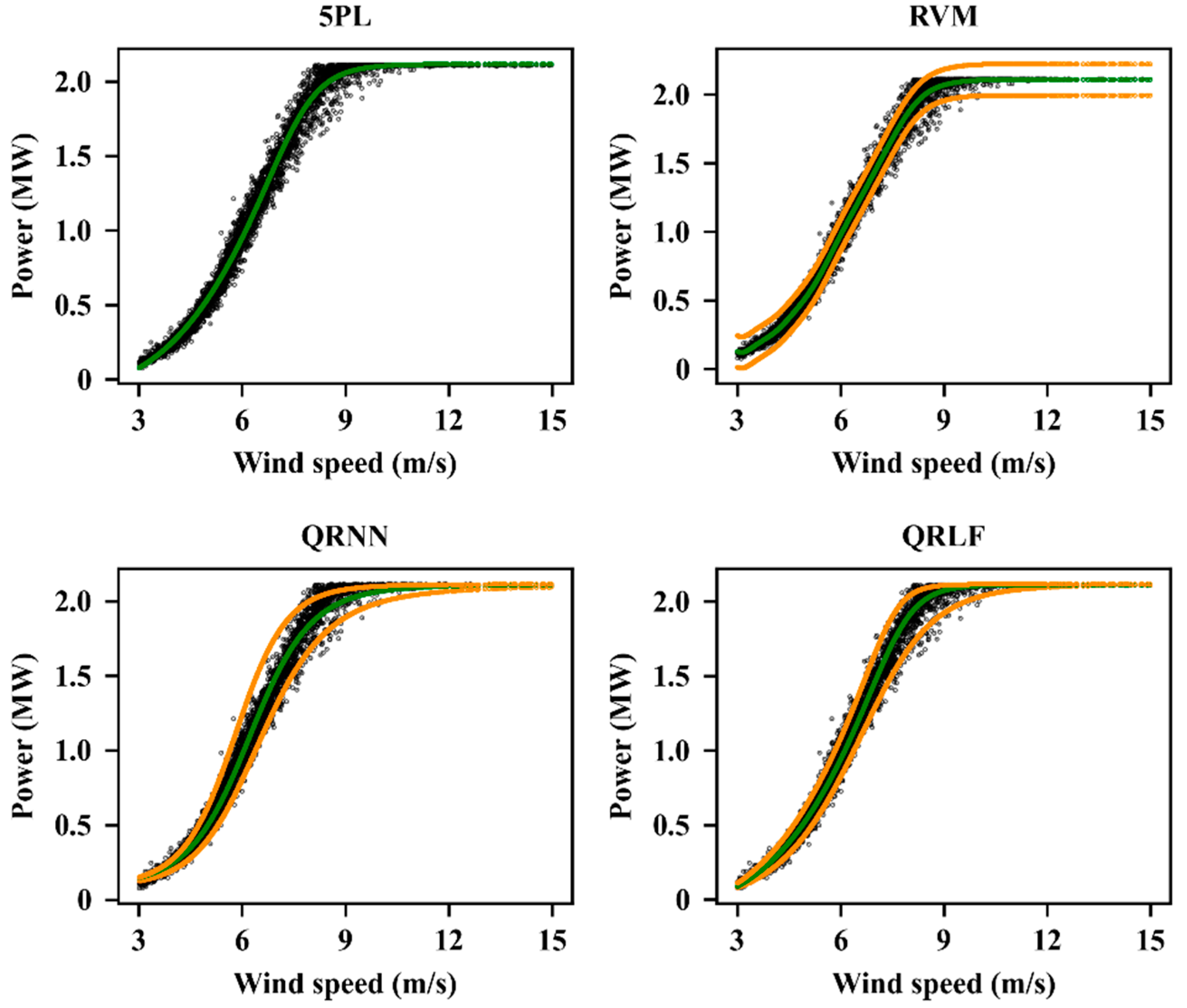
4.3.3. Results for WTPC Modelling

This part compares the proposed QRLF method (5P-QRLF optimized by PSO) with 5PL, RVM and QRNN to comprehensively evaluate the model performance. In order to avoid the impact of individual cases, we randomly select five wind turbines from each wind farm for testing. On the one hand, MAPE and NRMSE are utilized to evaluate the deterministic fitting accuracy of the aforementioned fitting methods; on the other hand, we use PICP, PINAW and NC to test the performance of the predicted CI.

Table 5. Fitting results of different wind turbine power curve (WTPC) modelling methods.

Wind Farm	Methods	MAPE	NRMSE	PICP90%	PINAW90%	NC90%
WF1 (2 MW)	5PL	6.26%	1.68%	N/A	N/A	N/A
	RVM	5.73%	1.62%	0.91	0.46	0.49
	QRNN	7.93%	1.83%	0.83	0.31	0.38
	QRLF	5.95%	1.65%	0.82	0.27	0.29
WF2 (2 MW)	5PL	11.44%	2.21%	N/A	N/A	N/A
	RVM	9.12%	2.19%	0.90	0.81	0.89
	QRNN	15.88%	2.34%	0.79	0.43	0.54
	QRLF	9.28%	2.19%	0.91	0.36	0.39
WF3 (5 MW)	5PL	10.28%	1.72%	N/A	N/A	N/A
	RVM	8.05%	1.65%	0.88	0.61	0.69
	QRNN	13.99%	2.49%	0.61	0.39	0.67
	QRLF	8.84%	1.72%	0.93	0.39	0.42

lists the average values of the fitting results of each wind farm, and Figure 9 shows the detailed information of one of the test wind turbines.

In Table 5, 5PL is selected as the benchmark for deterministic WTPC modelling because it has been proved to have good fitting accuracy in previous studies [9]. As mentioned in Section 2.1, 5PL can only be utilized for deterministic curve fitting, therefore, we cannot obtain the PICP_90%, PINAW_90% and NC_90% of 5PL. RVM is selected because it can significantly increase the calculation speed while maintaining the fitting accuracy of GP [27]. We can make the following conclusions from the test results listed in Table 5. (1) both RVM and QRLF have good nonlinear mapping ability in deterministic power curve fitting, and their average MAPE and NRMSE are lower than the benchmark (5PL). (2) For interval predictions, QRLF can significantly reduce the width of predicted CI, while maintaining high coverage probabilities. As listed in Table 5, the proposed method has almost the highest PICP_90% and the lowest PINAW_90% compared with RVM and QRNN. As a result, the proposed QRLF provides the most suitable predicted CI and has the lowest NC_90%. (3) From the fitting results in Table 5, there is no obvious correlation between the fitting accuracy and the installed capacity of wind turbine. Moreover, the performance rankings of the aforementioned fitting methods have not changed with the wind turbine installed capacity. More details can be obtained from Figure 9.

In Figure 9, during the training process, RVM assumes that the wind power follows the same Gaussian prior distribution, and thus the predicted CI in different wind speed ranges have similar width. However, the actual power output does not follow a specific distribution, which leads to a deviation between the predicted CI and the measured power output, especially when the wind speed is around the cut-in wind speed or exceeds the rated wind speed. Although QRNN can provide interval predictions without considering the prior distribution of wind power, the predicted CI calculated by QRLF is more suitable, especially in the wind speed range near the rated wind speed.

4.4. Discussions

At present, the proposed WTPC modelling method still has some limitations and needs to be improved. (1) Currently, the wind farm operators have not provided us with the detailed installation location of each wind turbine. Therefore, it is difficult to avoid the impact of turbine wakes on WTPC modelling. If the training set contains a large amount of measured data under wake effect, the established power curve will be “lower” than the real power curve (without turbine wakes). (2) The fitting accuracy of QRLF is sensitive to the initial settings of PSO. On the one hand, as mentioned in Section 2.4.3, we can enhance the reliability of the fitting results via repeating the optimization algorithm, i.e., PSO, multiple times. On the other hand, for the same type of wind turbine, we can use the model parameters of a trained wind turbine as the initial model parameters of a wind turbine to be trained to decrease the probability of falling into the local optimum.

In future works, we plan to use a full year of SCADA for model training, and then study the seasonal effects on power curve modelling. In addition, we will optimize the QRLF based WTPC model according to the specific application scenarios, such as probabilistic wind power forecasting and blade icing detection.

5. Conclusions

This paper combines the asymmetric absolute value function from the QR cost function with LF and proposes a new method for WTPC modelling. We use PSO, WOA and Adam optimization algorithm, respectively, to optimize the proposed QRLF with different model parameters. The results show that 5P-QRLF optimized by PSO generally has the best fitting performance. Based on QRLF, an adaptive outlier filtering method is developed through the symmetrical relationship of power distribution. After filtering, both sparse outliers and stacked outliers are eliminated while normal power points are effectively preserved. Compared with DBSCAN-Filter, the filtering results of the proposed QRLF-Filter are more robust and easy to deploy in actual wind farms. At last, we make comparative studies of QRLF and three typical WTPC modelling methods by using SCADA data collected from three wind farms. The results demonstrate that QRLF can provide both accurate deterministic fitting curves and appropriate interval predictions in different wind speed ranges. Compared with RVM and QRNN, it can reduce the width of the predicted CI while maintaining high coverage probabilities.

References

1. Manwell, F.J.; McGowan, G.J. Wind Energy Explained, 3rd ed.; Wiley: Hoboken, NJ, USA, 2009. [Google Scholar]
2. Villanueva, D.; Feijóo, A. A review on wind turbine deterministic power curve models. Appl. Sci. 2020, 10, 4186. [Google Scholar] [CrossRef]
3. Carrillo, C.; Obando Montaño, A.F.; Cidrás, J.; Díaz-Dorado, E. Review of power curve modelling for wind turbines. Renew. Sustain. Energy Rev. 2013, 21, 572–581. [Google Scholar] [CrossRef]
4. Wang, Y.; Hu, Q.; Srinivasan, D.; Wang, Z. Wind power curve modeling and wind power forecasting with inconsistent data. IEEE Trans. Sustain. Energy 2019, 10, 16–25. [Google Scholar] [CrossRef]
5. IET. Wind turbines Part 12–1: Power performance measurements of electricity producing wind turbines. In IEC 61400-12-1; International Electrical Comission: Geneva, Switzerland, 2005. [Google Scholar]
6. Marčiukaitis, M.; Žutautaitė, I.; Martišauskas, L.; Jokšas, B.; Gecevičius, G.; Sfetsos, A. Non-linear regression model for wind turbine power curve. Renew. Energy 2017, 113, 732–741. [Google Scholar] [CrossRef]
7. Teyabeen, A.A.; Akkari, F.R.; Jwaid, A.E. Power curve modelling for wind turbines. In Proceedings of the UKSim–AMSS 19th International Conference on Modelling & Simulation, Cambridge, UK, 5–7 April 2017. [Google Scholar] [CrossRef] [Green Version]
8. Taslimi-Renani, E.; Modiri-Delshad, M.; Elias, M.F.M.; Rahim, N.A. Development of an enhanced parametric model for wind turbine power curve. Appl. Energy 2016, 177, 544–552. [Google Scholar] [CrossRef]
9. Villanueva, D.; Feijóo, A. Comparison of logistic functions for modeling wind turbine power curves. Electr. Power Syst. Res. 2018, 155, 281–288. [Google Scholar] [CrossRef]
10. Seo, S.; Oh, S.; Kwak, H. Wind turbine power curve modeling using maximum likelihood estimation method. Renew. Energy 2019, 136, 1164–1169. [Google Scholar] [CrossRef]
11. Lydia, M.; Selvakumar, A.I.; Kumar, S.S.; Kumar, G.E.P. Advanced algorithms for wind turbine power curve modeling. IEEE Trans. Sustain. Energy 2013, 4, 827–835. [Google Scholar] [CrossRef]
12. Kusiak, A.; Zheng, H.; Song, Z. Models for monitoring wind farm power. Renew. Energy 2009, 34, 583–590. [Google Scholar] [CrossRef]
13. Thapar, V.; Agnihotri, G.; Sethi, V.K. Critical analysis of methods for mathematical modelling of wind turbines. Renew. Energy 2011, 36, 3166–3177. [Google Scholar] [CrossRef]
14. Yesilbudak, M. Implementation of novel hybrid approaches for power curve modeling of wind turbines. Energy Convers. Manag. 2018, 171, 156–169. [Google Scholar] [CrossRef]
15. Manobel, B.; Sehnke, F.; Lazzús, J.A.; Salfate, I.; Felder, M.; Montecinos, S. Wind turbine power curve modeling based on Gaussian processes and artificial neural networks. Renew. Energy 2018, 125, 1015–1020. [Google Scholar] [CrossRef]
16. Schlechtingen, M.; Santos, I.F.; Achiche, S. Using data-mining approaches for wind turbine power curve monitoring: A comparative study. IEEE Trans. Sustain. Energy 2013, 4, 671–679. [Google Scholar] [CrossRef]
17. Janssens, O.; Noppe, N.; Devriendt, C.; Walle, R.V.D.; Hoecke, S.V. Data-driven multivariate power curve modeling of offshore wind turbines. Eng. Appl. Artificial Intel. 2016, 55, 331–338. [Google Scholar] [CrossRef]
18. Yan, J.; Zhang, H.; Liu, Y.; Han, S.; Li, L. Uncertainty estimation for wind energy conversion by probabilistic wind turbine power curve modelling. Appl. Energy 2019, 239, 1356–1370. [Google Scholar] [CrossRef]
19. Pandit, R.K.; Infield, D. Using Gaussian process theory for wind turbine power curve analysis with emphasis on the confidence Intervals. In Proceedings of the 6th International Conference on Clean Electrical Power (ICCEP), Santa Margherita Ligure, Italy, 27–29 June 2017. [Google Scholar] [CrossRef] [Green Version]
20. Guo, P.; Infield, D. Wind turbine power curve modeling and monitoring with Gaussian process and SPRT. IEEE Trans. Sustain. Energy 2020, 11, 107–115. [Google Scholar] [CrossRef] [Green Version]
21. Rogers, T.J.; Gardner, P.; Dervilis, N. Probabilistic modelling of wind turbine power curves with application of heteroscedastic Gaussian process regression. Renew. Energy 2020, 148, 1124–1136. [Google Scholar] [CrossRef]
22. Virgolino, G.C.M.; Mattos, C.L.C.; Magalhães, J.A.F.; Barreto, G.A. Gaussian processes with logistic mean function for modeling wind turbine power curves. Renew. Energy 2020, 162, 458–465. [Google Scholar] [CrossRef]
23. Pandit, R.K.; Infield, D.; Kolios, A. Gaussian process power curve models incorporating wind turbine operational variables. Energy Rep. 2020, 6, 1658–1669. [Google Scholar] [CrossRef]
24. Astolfi, D.; Castellani, F.; Lombardi, A.; Terzi, L. Multivariate SCADA data analysis methods for real-world wind turbine power curve monitoring. Energies 2021, 14, 1105. [Google Scholar] [CrossRef]
25. Pandit, R.K.; Kolios, A. SCADA data-based support vector machine wind turbine power curve uncertainty estimation and its comparative studies. Appl. Sci. 2020, 10, 8685. [Google Scholar] [CrossRef]
26. Hu, Y.; Qiao, Y.; Liu, J. Adaptive confidence boundary modeling of wind turbine power curve using SCADA data and its application. IEEE Trans. Sustain. Energy 2019, 10, 1330–1341. [Google Scholar] [CrossRef]
27. Jing, B.; Qian, Z.; Wang, A.; Chen, T.; Zhang, F. Wind Turbine Power Curve Modelling Based on Hybrid Relevance Vector Machine. In Proceedings of the 4th International Symposium on Green Energy and Smart Grid, Xi’an, China, 20–22 August 2020. [Google Scholar] [CrossRef]
28. Park, J.Y.; Lee, J.K.; Oh, K.Y.; Lee, J.S. Development of a novel power curve monitoring method for wind turbines and its field tests. IEEE Trans. Energy Convers. 2014, 29, 119–128. [Google Scholar] [CrossRef]
29. Koenker, R.; Hallock, K.F. Quantile regression. J. Econ. Perpect. 2001, 15, 143–156. [Google Scholar] [CrossRef]
30. He, Y.; Zhang, W. Probability density forecasting of wind power based on multi-core parallel quantile regression neural network. Knowl. Based Syst. 2020, 209, 106431. [Google Scholar] [CrossRef]
31. Pei, S.; Li, Y. Wind turbine power curve modeling with a hybrid machine learning technique. Appl. Sci. 2019, 9, 4930. [Google Scholar] [CrossRef] [Green Version]
32. Zhao, Y.; Ye, L.; Wang, W.; Sun, H.; Ju, Y.; Tang, Y. Data-driven correction approach to refine power curve of wind farm under wind curtailment. IEEE Trans. Sustain. Energy 2018, 9, 95–105. [Google Scholar] [CrossRef]
33. Pandit, R.K.; Infield, D. SCADA-based wind turbine anomaly detection using Gaussian process models for wind turbine condition monitoring purposes. IET Renew. Power Gen. 2018, 12, 1249–1255. [Google Scholar] [CrossRef] [Green Version]
34. Gottschalk, P.G.; Dunn, J.R. The five-parameter logistic: A characterization and comparison with the four-parameter logistic. Anal. Biochem. 2005, 343, 54–65. [Google Scholar] [CrossRef]
35. He, Y.; Li, H.; Wang, S.; Yao, X. Uncertainty analysis of wind power probability density forecasting based on cubic spline interpolation and support vector quantile regression. Neurocomputing 2020, 430, 121–137. [Google Scholar] [CrossRef]
36. Mirjalili, S.; Lewis, A. The whale optimization algorithm. Adv. Eng. Softw. 2016, 95, 51–67. [Google Scholar] [CrossRef]
37. Kennedy, J.; Eberhart, R. Particle Swarm Optimization. In Proceedings of the IEEE International Conference on Neural Networks, Perth, Australia, 27 November–1 December 1995. [Google Scholar] [CrossRef]
38. Shi, Y.; Eberhart, R. A modified particle swarm optimizer. In Proceedings of the IEEE International Conference on Evolutionary Computation, Anchorage, AK, USA, 4–9 May 1998. [Google Scholar] [CrossRef]
39. Kingma, D.P.; Ba, J.L. Adam: A method for stochastic optimization. In Proceedings of the 3rd International Conference on Learning Representations, San Diego, CA, USA, 7–9 May 2015. [Google Scholar]
40. Quan, H.; Srinivasan, D.; Khosravi, A. Uncertainty handling using neural network-based prediction intervals for electrical load forecasting. Energy 2014, 73, 916–925. [Google Scholar] [CrossRef]
41. Zhang, Z.; Qin, H.; Liu, Y.; Yao, L.; Yu, X.; Lu, J.; Jiang, Z.; Feng, Z. Wind speed forecasting based on quantile regression minimal gated memory network and kernel density estimation. Energy Convers. Manag. 2019, 196, 1395–1409. [Google Scholar] [CrossRef]
Figure 1. Scatter plot of wind speed and power output of a wind turbine.
Applsci 11 03048 g001
Figure 2. Flow chart of the proposed outlier filtering method.
Applsci 11 03048 g002
Figure 3. Fitting results of quantile regression (QRLF) with different quantiles: (a) wind turbine without wind curtailment; (b) wind turbine under wind curtailment.
Applsci 11 03048 g003
Figure 4. Results of outlier filtering, where the black points are power points after outlier filtering, and the red points are power outliers.
Applsci 11 03048 g004
Figure 5. The relationship between d1/d2, and the number of iterations, where the red line is the threshold for the end condition of outlier filtering.
Applsci 11 03048 g005
Figure 6. The values of quantile regression (QR) cost function optimized by particle swarm optimization (PSO), whale optimization algorithm (WOA) and Adam algorithms during the training process.
Applsci 11 03048 g006
Figure 7. Scatter plots of wind speed and power output of WT02, WT08 and WT10., where the black points are the raw data of power outputs, and the orange points are the power outputs after outlier filtering.
Applsci 11 03048 g007
Figure 8. Results of outlier filtering by GP-Filter, DBSCAN-Filter and QRLF-Filter, where the black points are the raw data of power outputs, and the orange points are the power outputs after outlier filtering.
Applsci 11 03048 g008
Figure 9. Fitting results of WT03 in WF1 where the black points are the measured power outputs, the green curves are the deterministic fitting curves and the orange curves are the boundaries of the predicted CI.
Applsci 11 03048 g009