
Global Study of Human Heart Rhythm Synchronization with the Earth’s Time Varying Magnetic Field


 ,
,
Abstract
:1. Introduction
1.1. Literature Overview
1.2. Motivation
2. Materials and Methods
2.1. Participants
2.2. HRV Data Collection
2.3. Magnetic Field Data
2.4. Heart Lock-In Procedure
2.5. Computation of the Power of the Local Magnetic Field
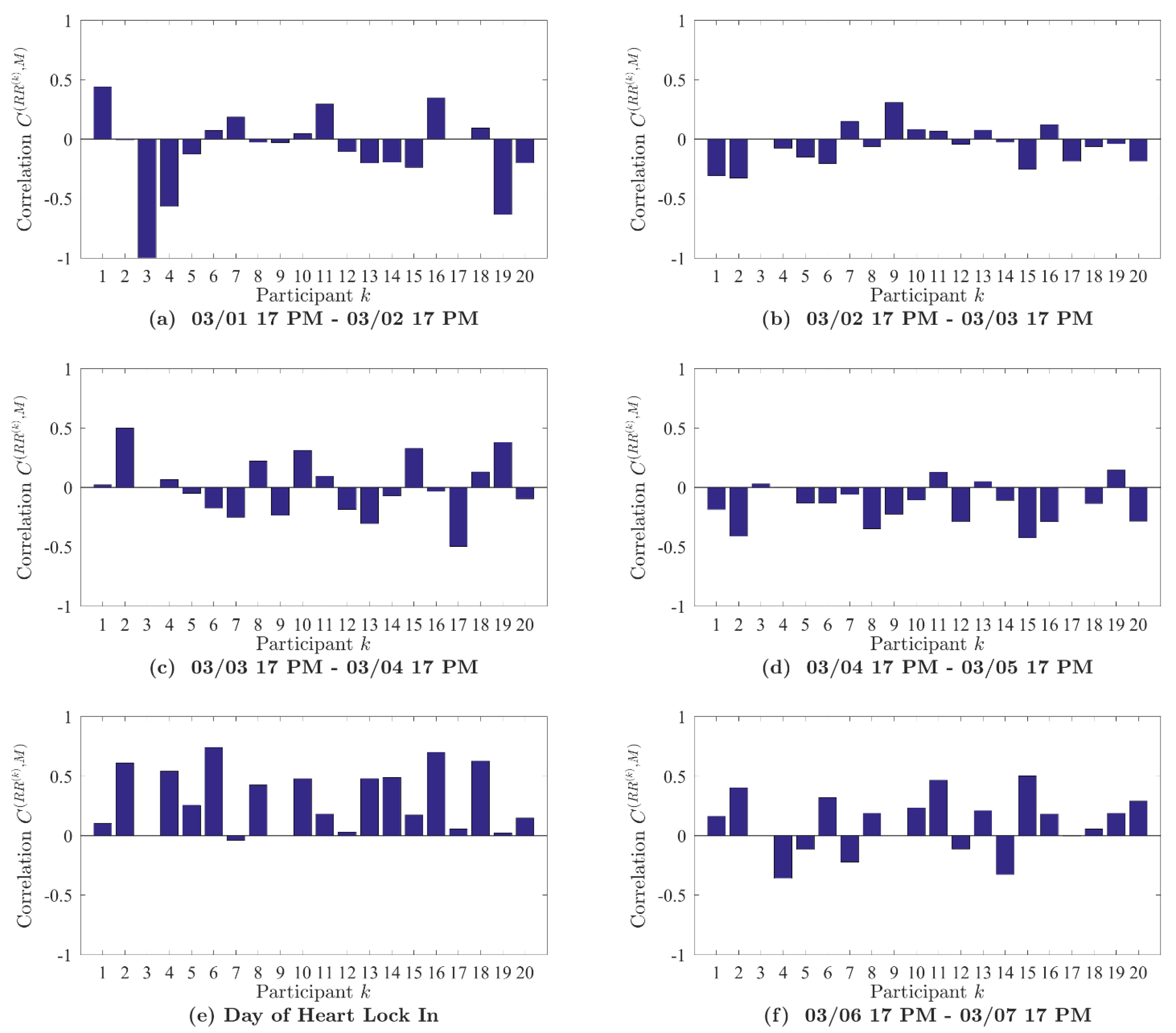
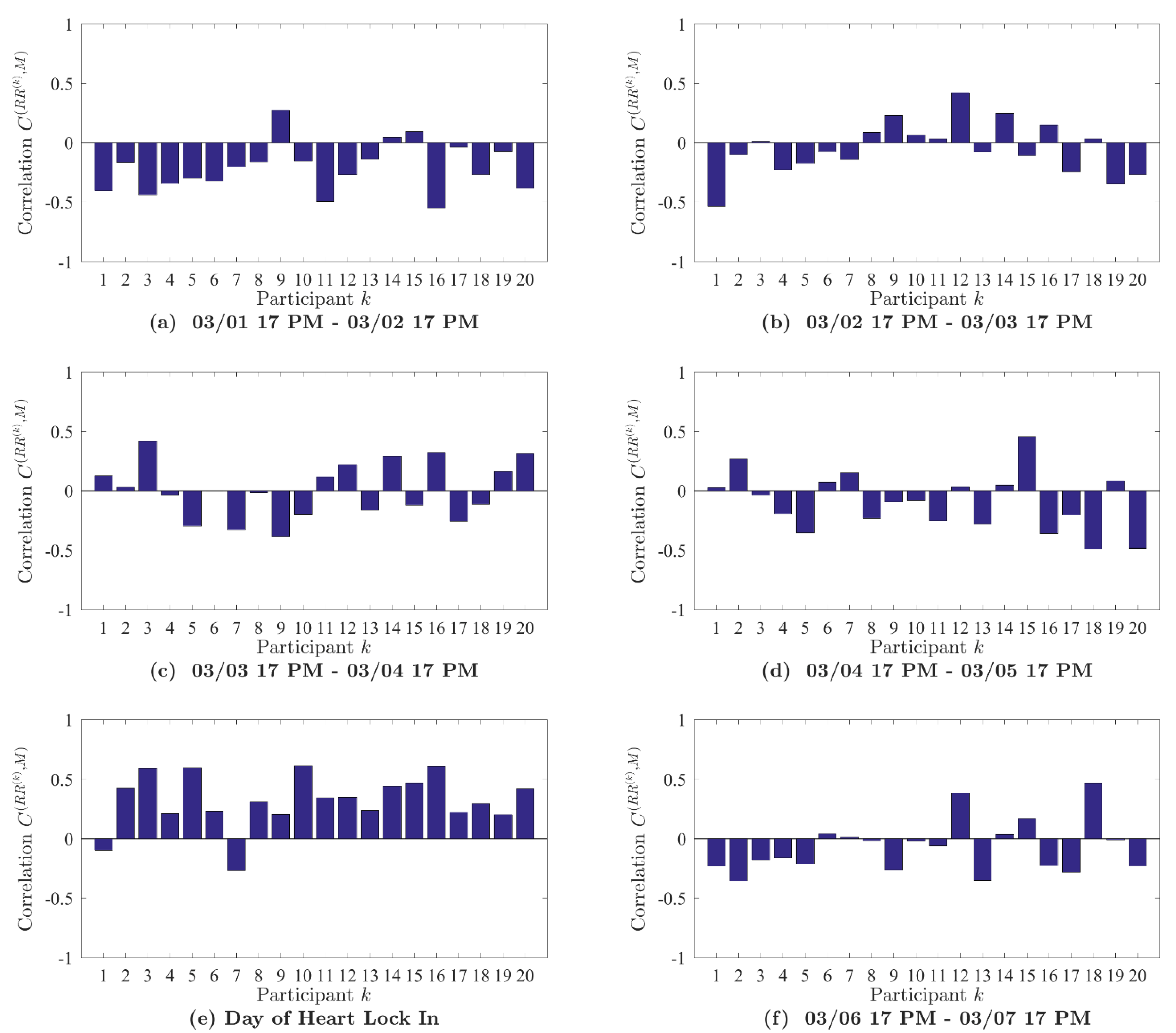
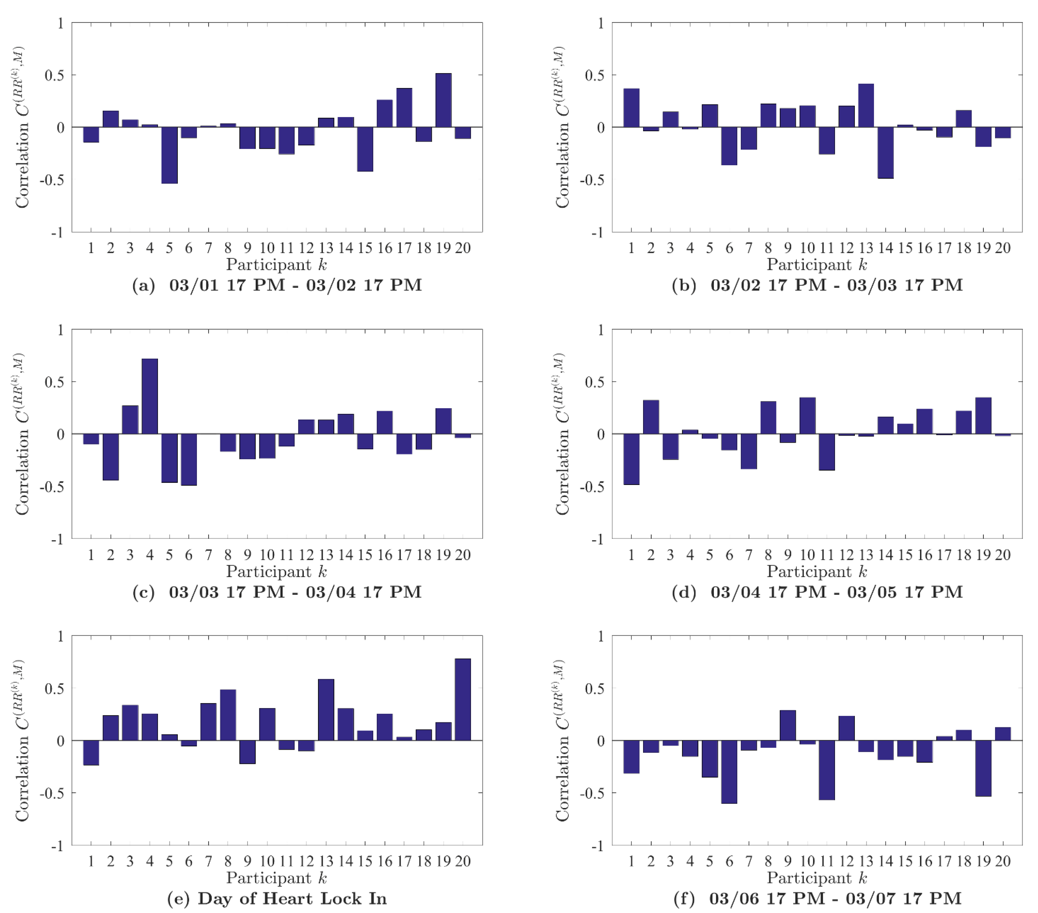
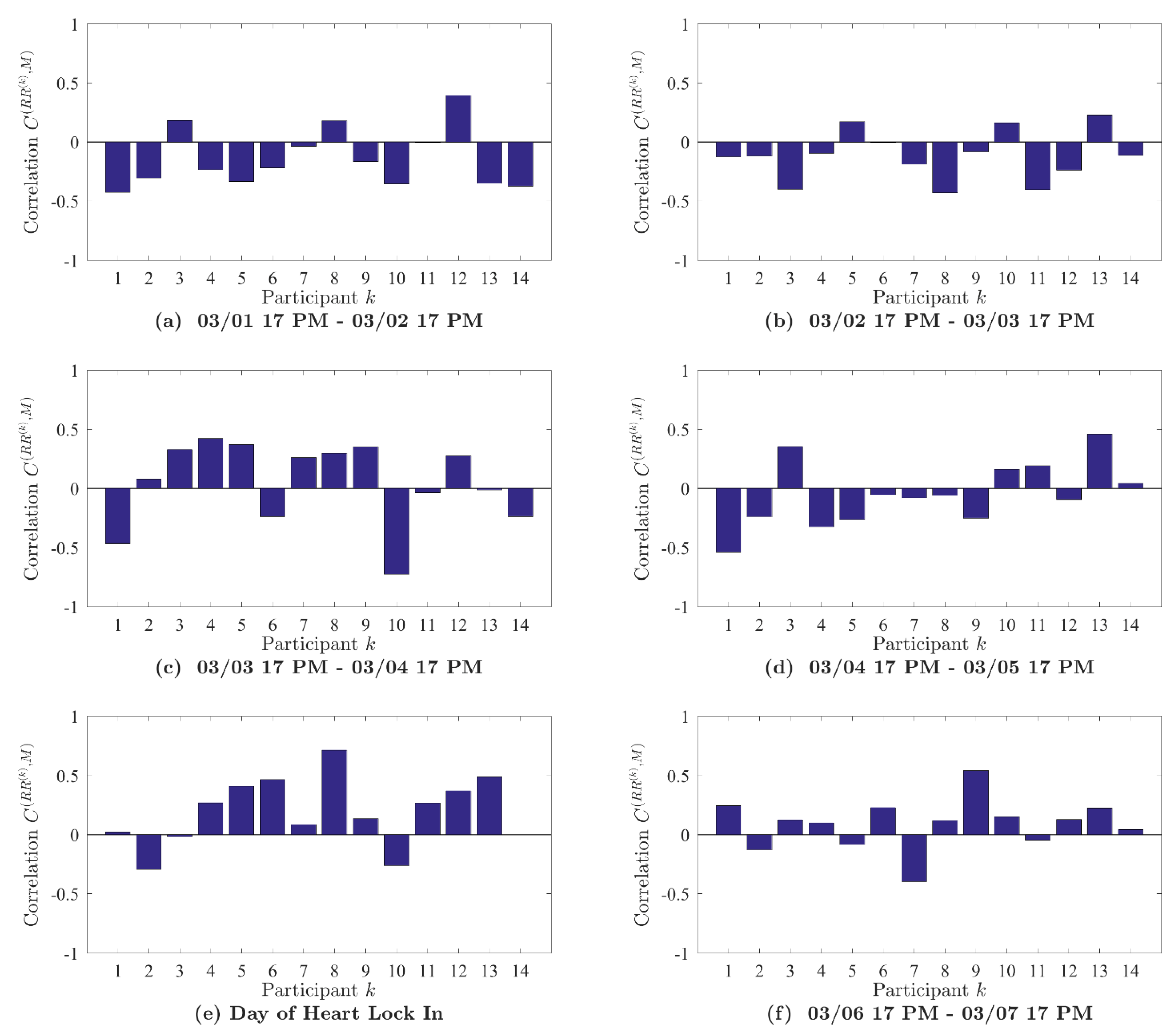
2.6. Synchronization between Participants’ HRV and Earth’s Magnetic Field
- Data signals RR and M are divided into T 5-min-long observation windows (according to HRV analysis standards) [36] and optimal time lag values are computed for each observation window (using the procedure presented in [11] and summarized above) for HRV time series and magnetic field spectral power data signal . This procedure maps RR and M data series to integer vectors, describing dynamical and geometrical properties of those series.
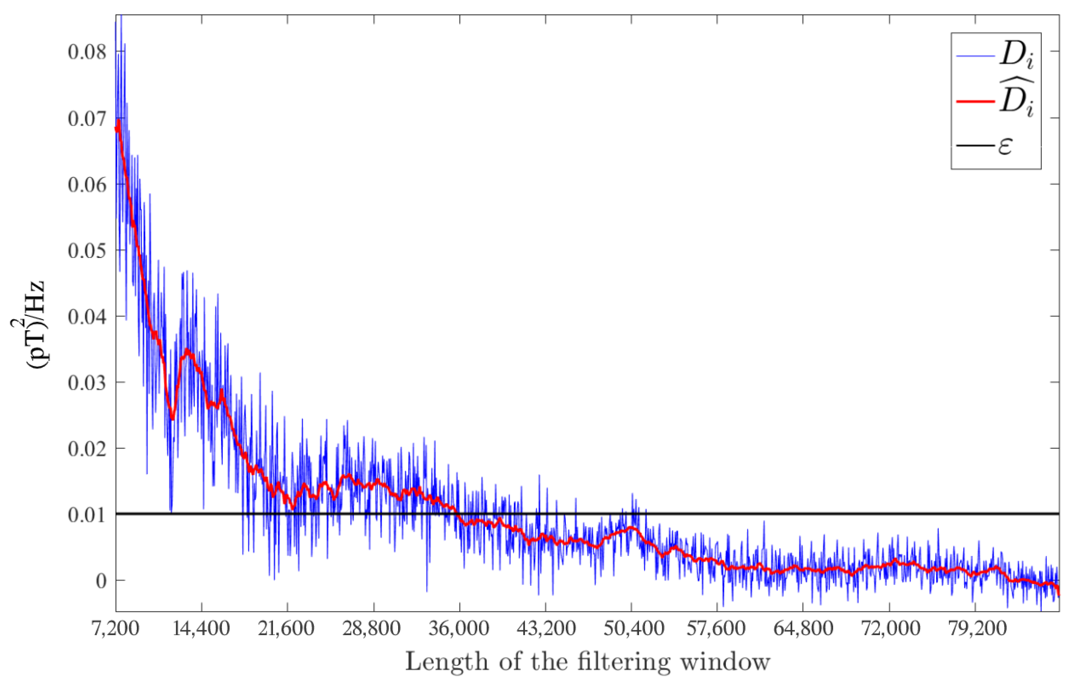
- Obtained optimal time lag vectors are smoothed via the computation of moving average in order to identify averaged changes in time lags for HRV and magnetic field data . The size of the observation window used for the moving average is 20 data points.
- Pearson correlation coefficient is calculated between averaged optimal time lag vectors. Resulting value is considered as the degree of synchronization between analyzed HRV and magnetic field spectral power signals. Naturally, higher value of corresponds to a higher degree of synchronization and vice versa (). Note that the assumption of the normality of data series used in further analysis was verified.
2.7. Statistical Analysis
- Pearson correlation significance test (Null Hypothesis ) is used in order to assess the statistical significance of the synchronization between participants’ HRV and Earth’s magnetic field obtained via the technique described in previous subsection.
- The Repeated Measures design is used with multiple measures of the same variable taken on the same subjects under different conditions or at two or more times. The assumption of sphericity was tested using Mauchly’s Test of Sphericity, any violations of the assumption that occurred are noted in the results tables along with their correction procedure. When used, post hoc multiple comparison tests were corrected with the Bonferroni test that adjusts the observed significance level for the fact that multiple comparisons were made. In this study, Repeated Measures ANOVA was used to examine differences in the mean LMF-HRV-correlations over time. It was also used to test for differences in HRV coherence, and heart rhythm synchronization before, during and after practice of the Heart Lock-In technique.
2.8. Analysis of Synchronization between Participants’ HRV and Local Magnetic Field Power
3. Results
3.1. Analysis of Heart Rhythm Coherence during the Heart Lock-In
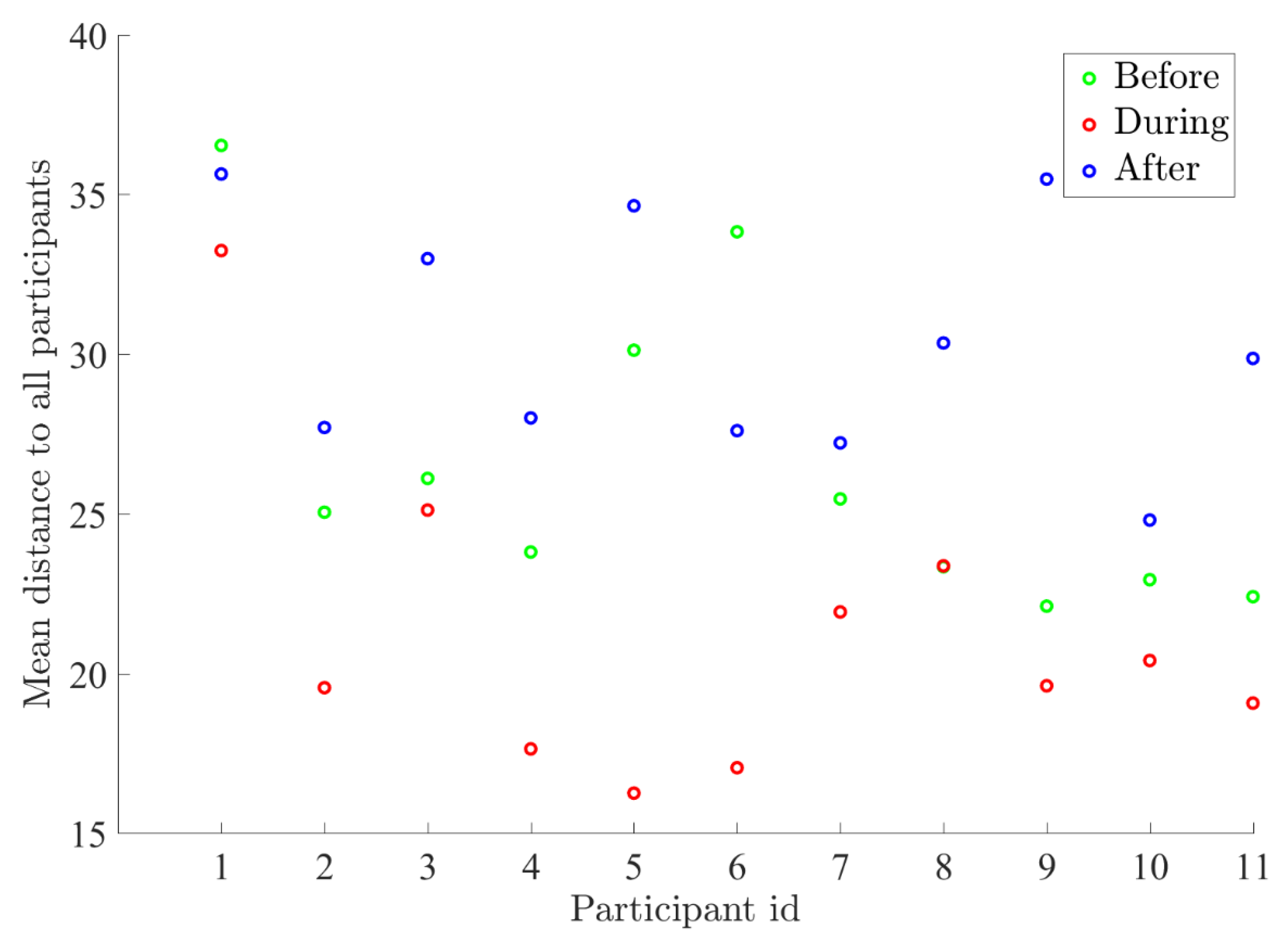
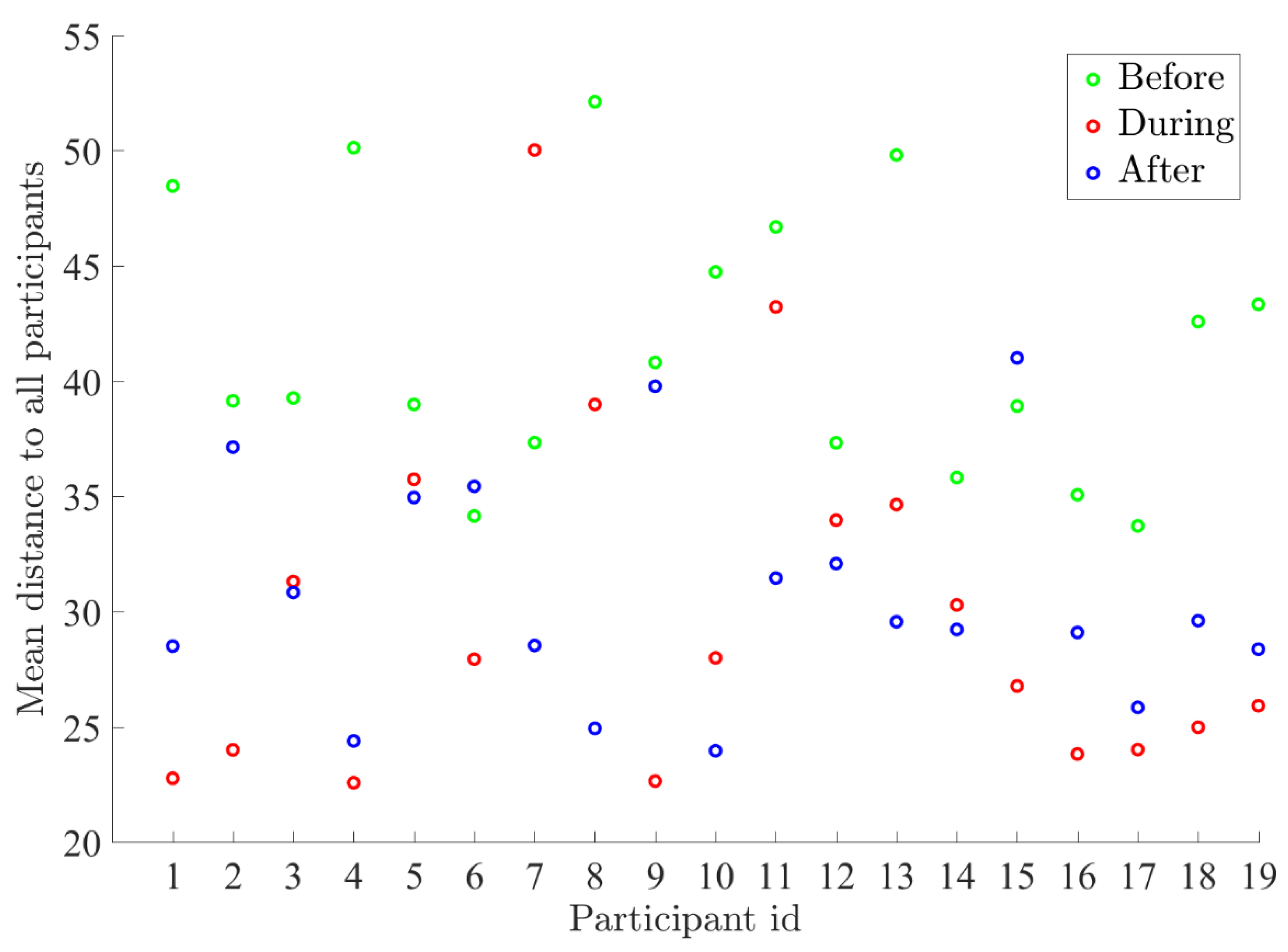
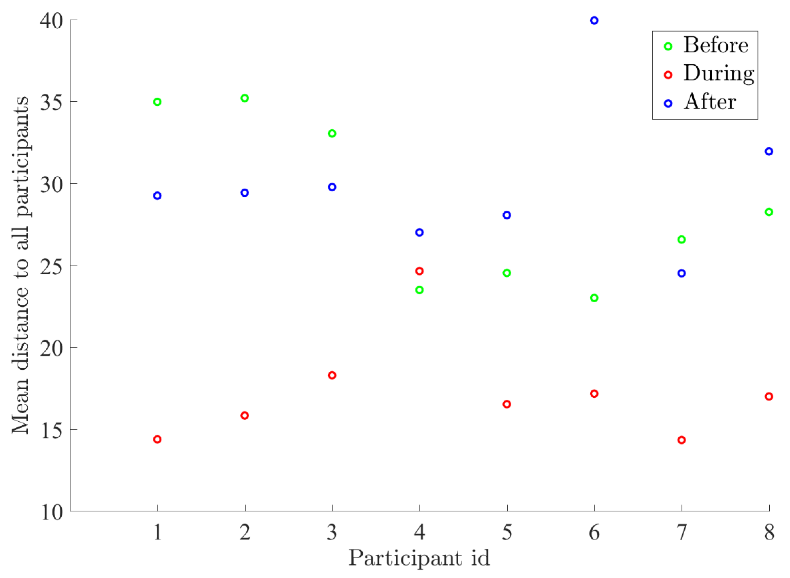
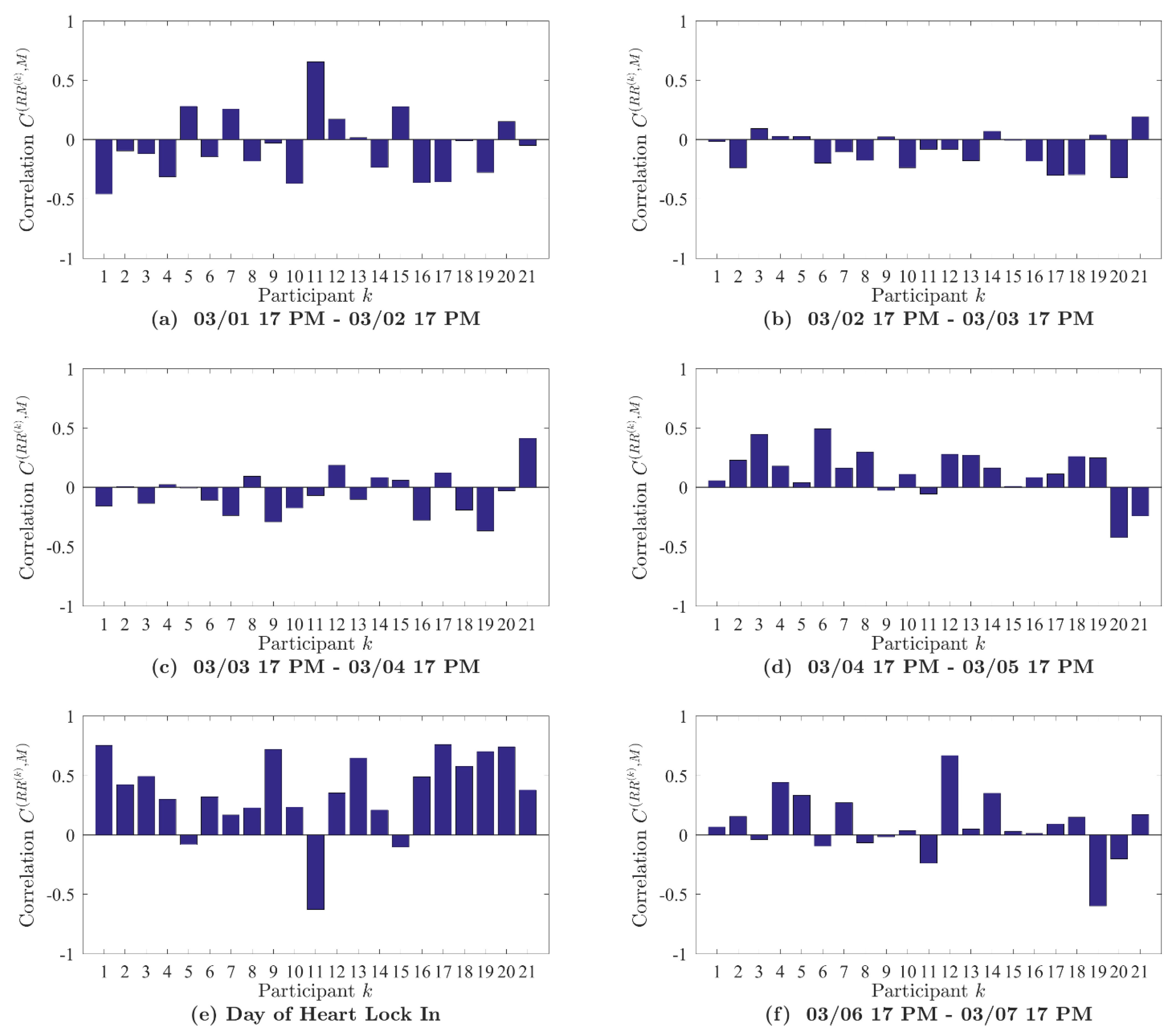
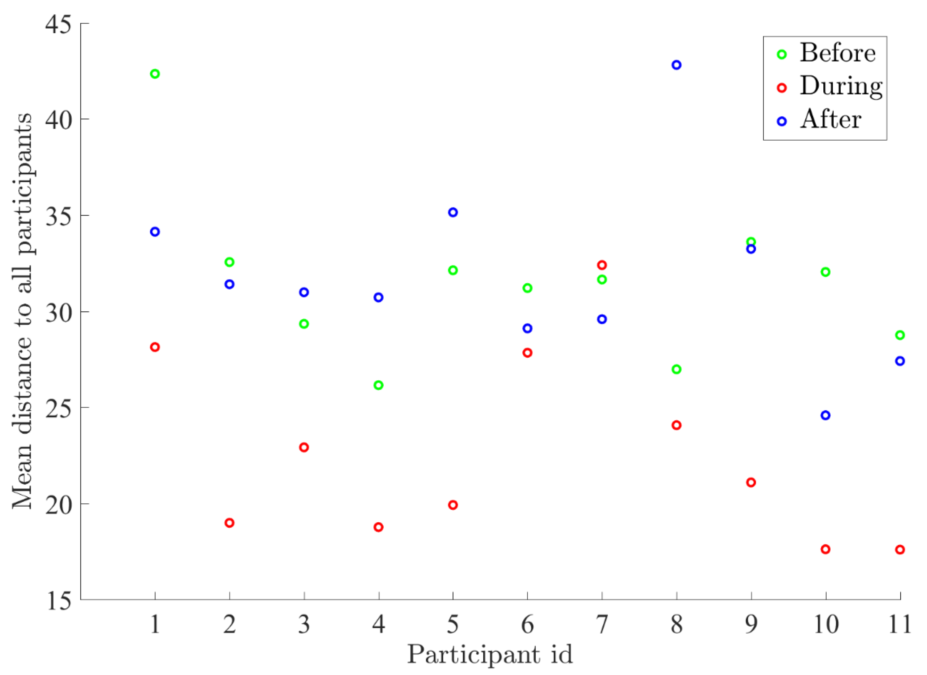
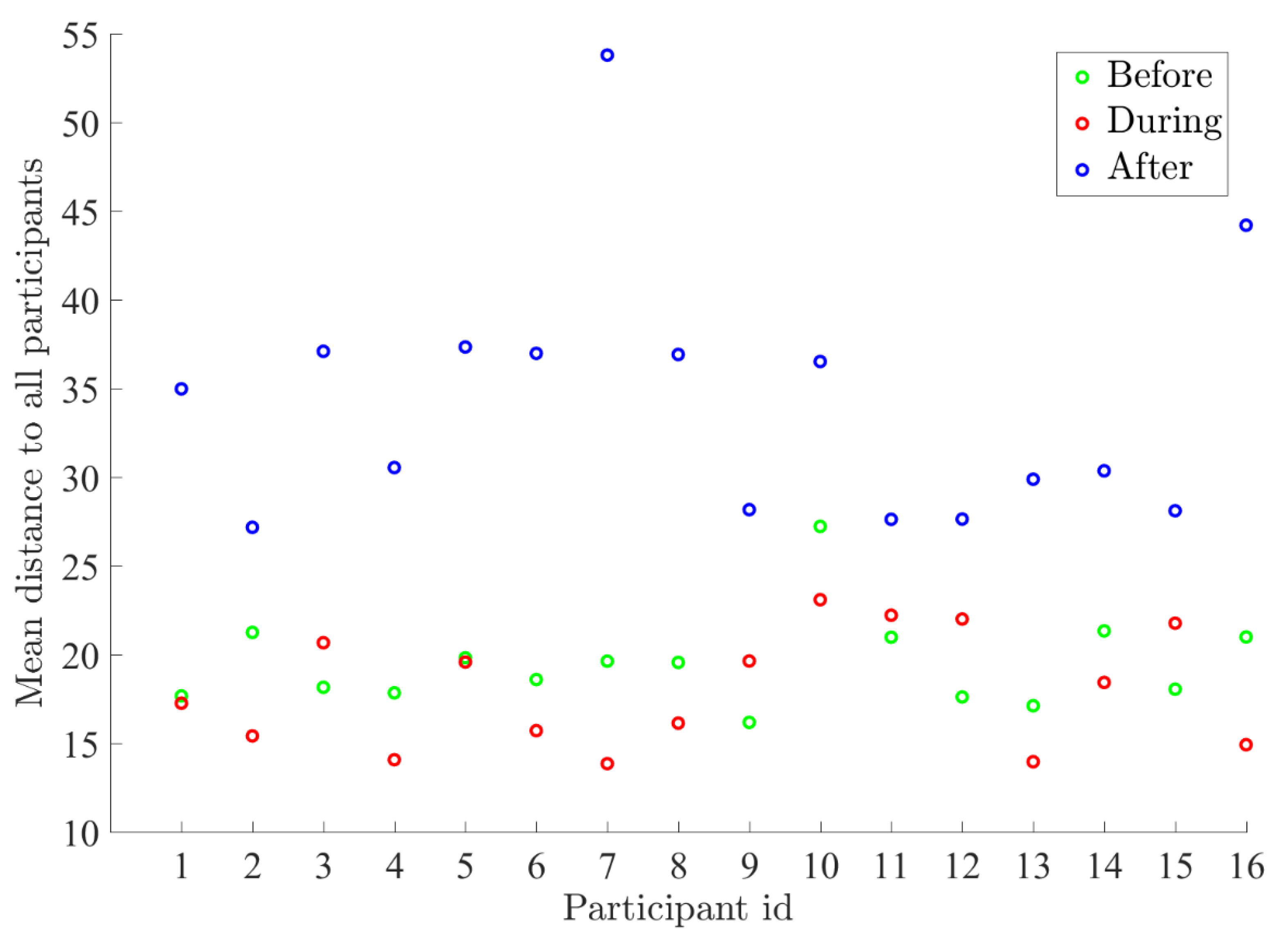
3.2. Analysis of Pairwise HRV Synchronization between Group Members
4. Discussion
Limitations and Suggestions for Future Studies
5. Conclusions
Author Contributions
Funding
Institutional Review Board Statement
Informed Consent Statement
Data Availability Statement
Acknowledgments
Conflicts of Interest
Appendix A

Appendix B


References
- Cornélissen, G.; Halberg, F.; Schwartzkopff, O.; Delmore, P.; Katinas, G.; Hunter, D.; Tarquini, B.; Tarquini, R.; Perfetto, F.; Watanabe, Y.; et al. Chronomes, time structures, for chronobioengineering for “a full life”. Biomed. Instrum. Technol. 1999, 33, 152–187. [Google Scholar]
- Qin, S.; Yin, H.; Yang, C.; Dou, Y.; Liu, Z.; Zhang, P.; Yu, H.; Huang, Y.; Feng, J.; Hao, J.; et al. A magnetic protein biocompass. Nat. Mater. 2016, 15, 217–226. [Google Scholar] [CrossRef]
- Price, C.; Williams, E.; Elhalel, G.; Sentman, D. Natural ELF fields in the atmosphere and in living organisms. Int. J. Biometeorol. 2020, 65, 85–928. [Google Scholar] [CrossRef]
- Kuzmenko, N.; Shchegolev, B.; Pliss, M.; Tsyrlin, V. The Influence of Weak Geomagnetic Disturbances on the Rat Cardiovascular System under Natural and Shielded Geomagnetic Field Conditions. Biophysics 2019, 64, 109–116. [Google Scholar] [CrossRef]
- Otsuka, K.; Cornelissen, G.; Norboo, T.; Takasugi, E.; Halberg, F. Chronomics and “glocal”(combined global and local) assessment of human life. Prog. Theor. Phys. Suppl. 2008, 173, 134–152. [Google Scholar] [CrossRef]
- Dimitrova, S.; Stoilova, I.; Cholakov, I. Influence of local geomagnetic storms on arterial blood pressure. Bioelectromagn. J. Bioelectromagn. Soc. Soc. Phys. Regul. Biol. Med. Eur. Bioelectromagn. Assoc. 2004, 25, 408–414. [Google Scholar] [CrossRef] [PubMed]
- Hamer, J. Biological entrainment of the human brain by low frequency radiation. Northrop Space Labs 1965, 36, 65–199. [Google Scholar]
- Oraevskiĭ, V.; Breus, T.; Baevskiĭ, R.; Rapoport, S.; Petrov, V.; Barsukova, Z.; Rogoza, A. Effect of geomagnetic activity on the functional status of the body. Biofizika 1998, 43, 819. [Google Scholar] [PubMed]
- Pobachenko, S.; Kolesnik, A.; Borodin, A.; Kalyuzhin, V. The contingency of parameters of human encephalograms and Schumann resonance electromagnetic fields revealed in monitoring studies. Biophysics 2006, 51, 480–483. [Google Scholar] [CrossRef]
- Cornélissen, G.; Halberg, F.; Breus, T.; Syutkina, E.V.; Baevsky, R.; Weydahl, A.; Watanabe, Y.; Otsuka, K.; Siegelova, J.; Fiser, B.; et al. Non-photic solar associations of heart rate variability and myocardial infarction. J. Atmos. Sol. Terr. Phys. 2002, 64, 707–720. [Google Scholar] [CrossRef]
- Timofejeva, I.; McCraty, R.; Atkinson, M.; Joffe, R.; Vainoras, A.; Alabdulgader, A.A.; Ragulskis, M. Identification of a group’s physiological synchronization with earth’s magnetic field. Int. J. Environ. Res. Public Health 2017, 14, 998. [Google Scholar] [CrossRef] [Green Version]
- Wang, C.X.; Hilburn, I.A.; Wu, D.A.; Mizuhara, Y.; Cousté, C.P.; Abrahams, J.N.; Bernstein, S.E.; Matani, A.; Shimojo, S.; Kirschvink, J.L. Transduction of the geomagnetic field as evidenced from alpha-band activity in the human brain. Eneuro 2019. [Google Scholar] [CrossRef] [Green Version]
- Elhalel, G.; Price, C.; Fixler, D.; Shainberg, A. Cardioprotection from stress conditions by weak magnetic fields in the Schumann Resonance band. Sci. Rep. 2019, 9, 1–10. [Google Scholar] [CrossRef] [Green Version]
- Pishchalnikov, R.; Gurfinkel, Y.; Sarimov, R.; Vasin, A.; Sasonko, M.; Matveeva, T.; Binhi, V.; Baranov, M. Cardiovascular response as a marker of environmental stress caused by variations in geomagnetic field and local weather. Biomed. Signal Process. Control 2019, 51, 401–410. [Google Scholar] [CrossRef]
- Vieira, C.L.Z.; Alvares, D.; Blomberg, A.; Schwartz, J.; Coull, B.; Huang, S.; Koutrakis, P. Geomagnetic disturbances driven by solar activity enhance total and cardiovascular mortality risk in 263 US cities. Environ. Health 2019, 18, 83. [Google Scholar] [CrossRef] [PubMed] [Green Version]
- Otsuka, K.; Cornelissen, G.; Kubo, Y.; Shibata, K.; Mizuno, K.; Ohshima, H.; Furukawa, S.; Mukai, C. Anti-aging effects of long-term space missions, estimated by heart rate variability. Sci. Rep. 2019, 9, 1–12. [Google Scholar]
- Wickramasinghe, N.; Steele, E.J.; Wainwright, M.; Tokoro, G.; Fernando, M.; Qu, J. Sunspot Cycle Minima and Pandemics: The Case for Vigilance? JAsBO 2017, 5, 159. [Google Scholar]
- Doronin, V.; Parfentĕv, V.; Tleulin, S.; Namvar, R.; Somsikov, V.; Drobzhev, V.; Chemeris, A. Effect of variations of the geomagnetic field and solar activity on human physiological indicators. Biofizika 1998, 43, 647–653. [Google Scholar] [PubMed]
- Halberg, F.; Cornélissen, G.; McCraty, R.; Czaplicki, J.; Al-Abdulgader, A.A. Time structures (chronomes) of the blood circulation, populations’ health, human affairs and space weather. World Heart J. 2011, 3, 73. [Google Scholar]
- Khorseva, N. Using psychophysiological indices to estimate the effect of cosmophysical factors. Izv. Atmos. Ocean. Phys. 2013, 49, 839–852. [Google Scholar] [CrossRef]
- Khabarova, O.; Dimitrova, S. On the nature of people’s reaction to space weather and meteorological weather changes. Sun Geosph. 2009, 4, 60–71. [Google Scholar]
- Cornelissen Guillaume, G.; Gubin, D.; Beaty, L.A.; Otsuka, K. Some Near-and Far-Environmental Effects on Human Health and Disease with a Focus on the Cardiovascular System. Int. J. Environ. Res. Public Health 2020, 17, 3083. [Google Scholar] [CrossRef] [PubMed]
- McCraty, R.; Atkinson, M.; Stolc, V.; Alabdulgader, A.A.; Vainoras, A.; Ragulskis, M. Synchronization of human autonomic nervous system rhythms with geomagnetic activity in human subjects. Int. J. Environ. Res. Public Health 2017, 14, 770. [Google Scholar] [CrossRef] [PubMed] [Green Version]
- Alabdulgader, A.; McCraty, R.; Atkinson, M.; Dobyns, Y.; Vainoras, A.; Ragulskis, M.; Stolc, V. Long-term study of heart rate variability responses to changes in the solar and geomagnetic environment. Sci. Rep. 2018, 8, 1–14. [Google Scholar] [CrossRef] [PubMed] [Green Version]
- Shaffer, F.; McCraty, R.; Zerr, C.L. A healthy heart is not a metronome: An integrative review of the heart’s anatomy and heart rate variability. Front. Psychol. 2014, 5, 1040. [Google Scholar] [CrossRef] [Green Version]
- McCraty, R.; Shaffer, F. Heart rate variability: New perspectives on physiological mechanisms, assessment of self-regulatory capacity, and health risk. Glob. Adv. Health Med. 2015, 4, 46–61. [Google Scholar] [CrossRef] [Green Version]
- Thayer, J.F.; Hansen, A.L.; Saus-Rose, E.; Johnsen, B.H. Heart rate variability, prefrontal neural function, and cognitive performance: The neurovisceral integration perspective on self-regulation, adaptation, and health. Ann. Behav. Med. 2009, 37, 141–153. [Google Scholar] [CrossRef]
- McCraty, R.; Deyhle, A. The global coherence initiative: Investigating the dynamic relationship between people and earth’s energetic systems. Bioelectromagn. Subtle Energy Med. 2015, 2, 411–425. [Google Scholar]
- Persinger, M.A.; Saroka, K.S. Human quantitative electroencephalographic and Schumann Resonance exhibit real-time coherence of spectral power densities: Implications for interactive information processing. J. Signal Inf. Process. 2015, 6, 153. [Google Scholar] [CrossRef] [Green Version]
- Southwood, D. Some features of field line resonances in the magnetosphere. Planet. Space Sci. 1974, 22, 483–491. [Google Scholar] [CrossRef]
- Alfvén, H. Cosmical Electrodynamics; Ripol Classic: Moscow, Russia, 1963. [Google Scholar]
- Heacock, R. Two subtypes of type Pi micropulsations. J. Geophys. Res. 1967, 72, 3905–3917. [Google Scholar] [CrossRef]
- McPherron, R.L. Magnetic pulsations: Their sources and relation to solar wind and geomagnetic activity. Surv. Geophys. 2005, 26, 545–592. [Google Scholar] [CrossRef]
- Zenchenko, T.; Medvedeva, A.; Khorseva, N.; Breus, T. Synchronization of human heart-rate indicators and geomagnetic field variations in the frequency range of 0.5–3.0 mHz. Izv. Atmos. Ocean. Phys. 2014, 50, 736–744. [Google Scholar] [CrossRef]
- McCraty, R. New frontiers in heart rate variability and social coherence research: Techniques, technologies, and implications for improving group dynamics and outcomes. Front. Public Health 2017, 5, 267. [Google Scholar] [CrossRef] [Green Version]
- Novak, V.; Saul, J.P.; Eckberg, D.L. Task Force report on heart rate variability. Circulation 1997, 96, 1056. [Google Scholar]
- McCraty, R.; Tomasino, D. Emotional Stress, Positive Emotions, and Psychophysiological Coherence. In Stress in Health and Disease; Wiley-VCH: Hoboken, NJ, USA, 2006. [Google Scholar]
- McCraty, R.; Moor, S.; Goelitz, J.; Lance, S.W. Transforming Stress for Teens: The Heartmath Solution for Staying Cool under Pressure; Instant Help Books, an Imprint of New Harbinger Publications, Inc.: Oakland, CA, USA, 2016. [Google Scholar]
- Pearson, R.K.; Neuvo, Y.; Astola, J.; Gabbouj, M. The class of generalized hampel filters. In Proceedings of the IEEE 2015 23rd European Signal Processing Conference (EUSIPCO), Nice, France, 31 August–4 September 2015; pp. 2501–2505. [Google Scholar]
- Liu, Y. Noise reduction by vector median filtering. Geophysics 2013, 78, V79–V87. [Google Scholar] [CrossRef] [Green Version]
- Nykänen, V.; Groves, D.; Ojala, V.; Gardoll, S. Combined conceptual/empirical prospectivity mapping for orogenic gold in the northern Fennoscandian Shield, Finland. Aust. J. Earth Sci. 2008, 55, 39–59. [Google Scholar] [CrossRef]
- Mauring, E.; Kihle, O. Leveling aerogeophysical data using a moving differential median filter. Geophysics 2006, 71, L5–L11. [Google Scholar] [CrossRef]
- Hampel, F.R. A general qualitative definition of robustness. Ann. Math. Stat. 1971, 42, 1887–1896. [Google Scholar] [CrossRef]
- Timofejeva, I.; Poskuviene, K.; Cao, M.; Ragulskis, M. Synchronization measure based on a geometric approach to attractor embedding using finite observation windows. Complexity 2018, 2018, 8259496. [Google Scholar] [CrossRef]
- McCraty, R.; Atkinson, M.; Tomasino, D.; Bradley, R.T. The coherent heart heart-brain interactions, psychophysiological coherence, and the emergence of system-wide order. Integral Rev. A Transdiscipl. Transcult. J. New Thought Res. Prax. 2009, 5, 10–115. [Google Scholar]
- McCraty, R.; Atkinson, M.; Tiller, W.A.; Rein, G.; Watkins, A.D. The effects of emotions on short-term power spectrum analysis of heart rate variability. Am. J. Cardiol. 1995, 76, 1089–1093. [Google Scholar] [CrossRef]
- Tiller, W.A.; McCraty, R.; Atkinson, M. Cardiac coherence: A new, noninvasive measure of autonomic nervous system order. Altern. Ther. Health Med. 1996, 2, 52–65. [Google Scholar]
- Leon, E.; Clarke, G.; Callaghan, V.; Doctor, F. Affect-aware behaviour modelling and control inside an intelligent environment. Pervasive Mob. Comput. 2010, 6, 559–574. [Google Scholar] [CrossRef]
- Alabdulgade, A.; Maccraty, R.; Atkinson, M.; Vainoras, A.; Berškienė, K.; Mauricienė, V.; Daunoravičienė, A.; Navickas, Z.; Šmidtaitė, R.; Landauskas, M. Human heart rhythm sensitivity to earth local magnetic field fluctuations. J. Vibroeng. 2015, 17, 3271–3278. [Google Scholar]
- Morris, S.M. Achieving collective coherence: Group effects on heart rate variability, coherence and heart rhythm synchronization. Altern Ther Health Med 2010, 16, 62–72. [Google Scholar]
- Ragulskis, M.; Lukoseviciute, K. Non-uniform attractor embedding for time series forecasting by fuzzy inference systems. Neurocomputing 2009, 72, 2618–2626. [Google Scholar] [CrossRef]
- Lukoseviciute, K.; Ragulskis, M. Evolutionary algorithms for the selection of time lags for time series forecasting by fuzzy inference systems. Neurocomputing 2010, 73, 2077–2088. [Google Scholar] [CrossRef]


| Location | N | Age Mean, y | Age SD, y | Gender, % Female |
|---|---|---|---|---|
| United Kingdom | 14 | 39.2 | 12.3 | 57% |
| Lithuania | 20 | 23.3 | 0.6 | 80% |
| New Zealand | 22 | 42.7 | 10.1 | 50% |
| Saudi Arabia | 20 | 20.7 | 2.6 | 50% |
| California | 20 | 54.7 | 8.4 | 55% |
| All participants | 96 | 36.0 | 15.1 | 58.33% |
| N | Mean Sq. | df | F | p< | Partial | |
|---|---|---|---|---|---|---|
| California | 17 | 0.50 | 10 | 8.46 | 0.001 | 0.35 |
| Lithuania | 19 | 0.44 | 10 | 9.26 | 0.001 | 0.34 |
| New Zealand | 21 | 0.40 | 10 | 6.22 | 0.001 | 0.24 |
| Saudi Arabia | 19 | 0.18 | 10 | 2.62 | 0.01 | 0.13 |
| United Kingdom | 11 | 0.18 | 10 | 2.88 | 0.01 | 0.22 |
| California | |||||||||||
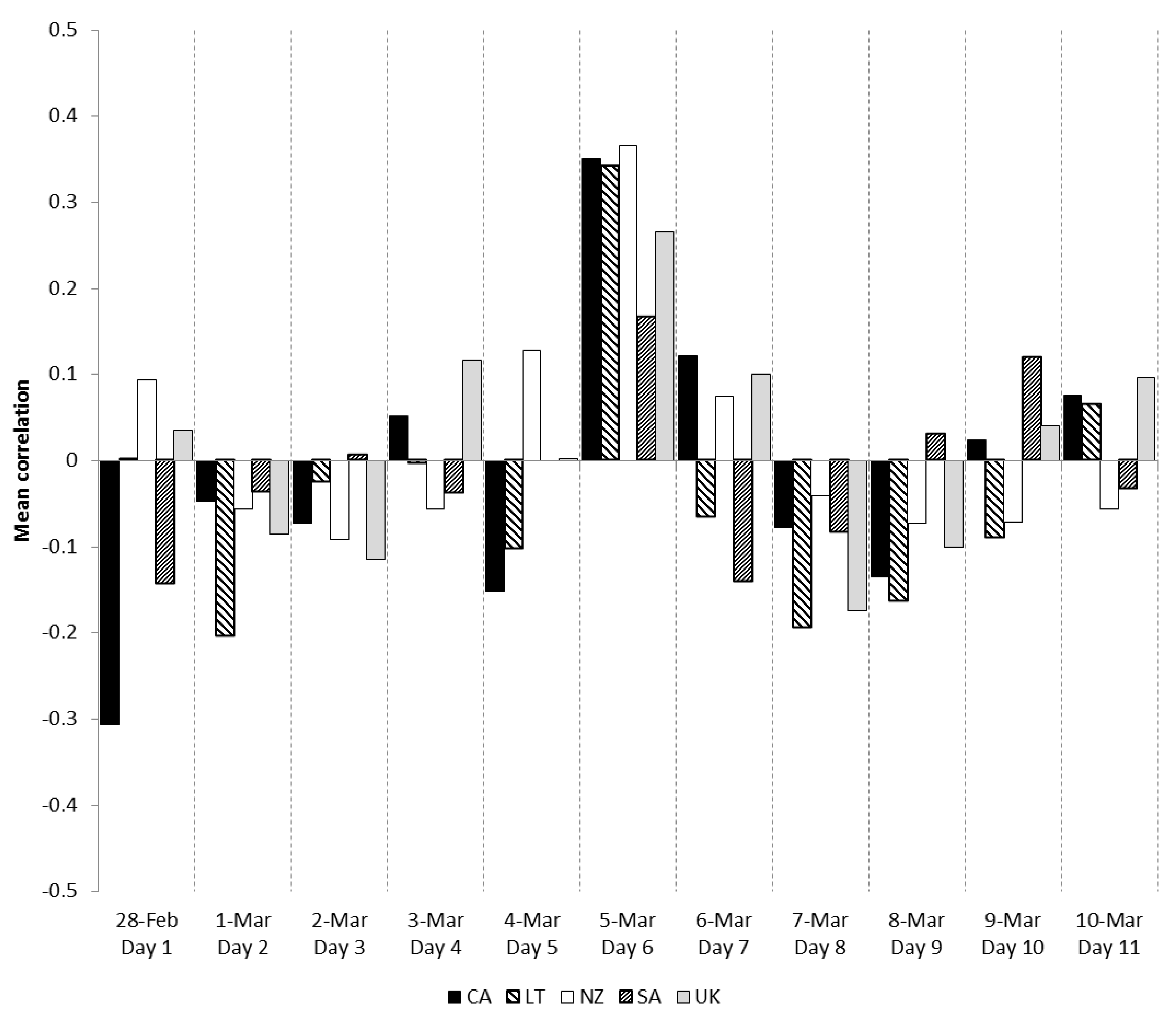
| Day | 28-February | 1-March | 2-March | 3-March | 4-March | 5-March | 6-March | 7-March | 8-March | 9-March | 10-March |
| Correlation | −0.297 | −0.056 | −0.068 | 0.058 | −0.139 | 0.335 | 0.115 | −0.070 | −0.127 | 0.017 | 0.088 |
| p value | 0.000 *** | 0.342 | 0.251 | 0.329 | 0.019 * | 0.000 *** | 0.053 | 0.236 | 0.031 * | 0.771 | 0.139 |
| Lithuania | |||||||||||
| Day | 28-February | 1-March | 2-March | 3-March | 4-March | 5-March | 6-March | 7-March | 8-March | 9-March | 10-March |
| Correlation | 0.001 | −0.214 | −0.051 | −0.004 | −0.096 | 0.320 | −0.074 | −0.201 | −0.146 | −0.101 | 0.047 |
| p value | 0.983 | 0.000 *** | 0.391 | 0.952 | 0.104 | 0.000 *** | 0.212 | 0.001 *** | 0.013 * | 0.088 | 0.430 |
| New Zealand | |||||||||||
| Day | 28-February | 1-March | 2-March | 3-March | 4-March | 5-March | 6-March | 7-March | 8-March | 9-March | 10-March |
| Correlation | 0.094 | −0.056 | −0.092 | −0.056 | 0.128 | 0.366 | 0.075 | −0.041 | −0.073 | −0.071 | −0.056 |
| p value | 0.114 | 0.345 | 0.120 | 0.348 | 0.031 * | 0.000 *** | 0.205 | 0.495 | 0.220 | 0.232 | 0.344 |
| Saudi Arabia | |||||||||||
| Day | 28-February | 1-March | 2-March | 3-March | 4-March | 5-March | 6-March | 7-March | 8-March | 9-March | 10-March |
| Correlation | −0.114 | −0.033 | 0.017 | −0.044 | 0.005 | 0.183 | −0.137 | −0.083 | 0.045 | 0.114 | −0.043 |
| p value | 0.054 | 0.574 | 0.769 | 0.455 | 0.928 | 0.002 ** | 0.020 * | 0.161 | 0.446 | 0.053 | 0.469 |
| United Kingdom | |||||||||||
| Day | 28-February | 1-March | 2-March | 3-March | 4-March | 5-March | 6-March | 7-March | 8-March | 9-March | 10-March |
| Correlation | 0.042 | −0.096 | −0.125 | 0.128 | 0.010 | 0.254 | 0.090 | −0.184 | −0.138 | 0.054 | 0.086 |
| p value | 0.481 | 0.106 | 0.034 * | 0.031 * | 0.870 | 0.000 *** | 0.130 | 0.002 ** | 0.019 * | 0.364 | 0.148 |
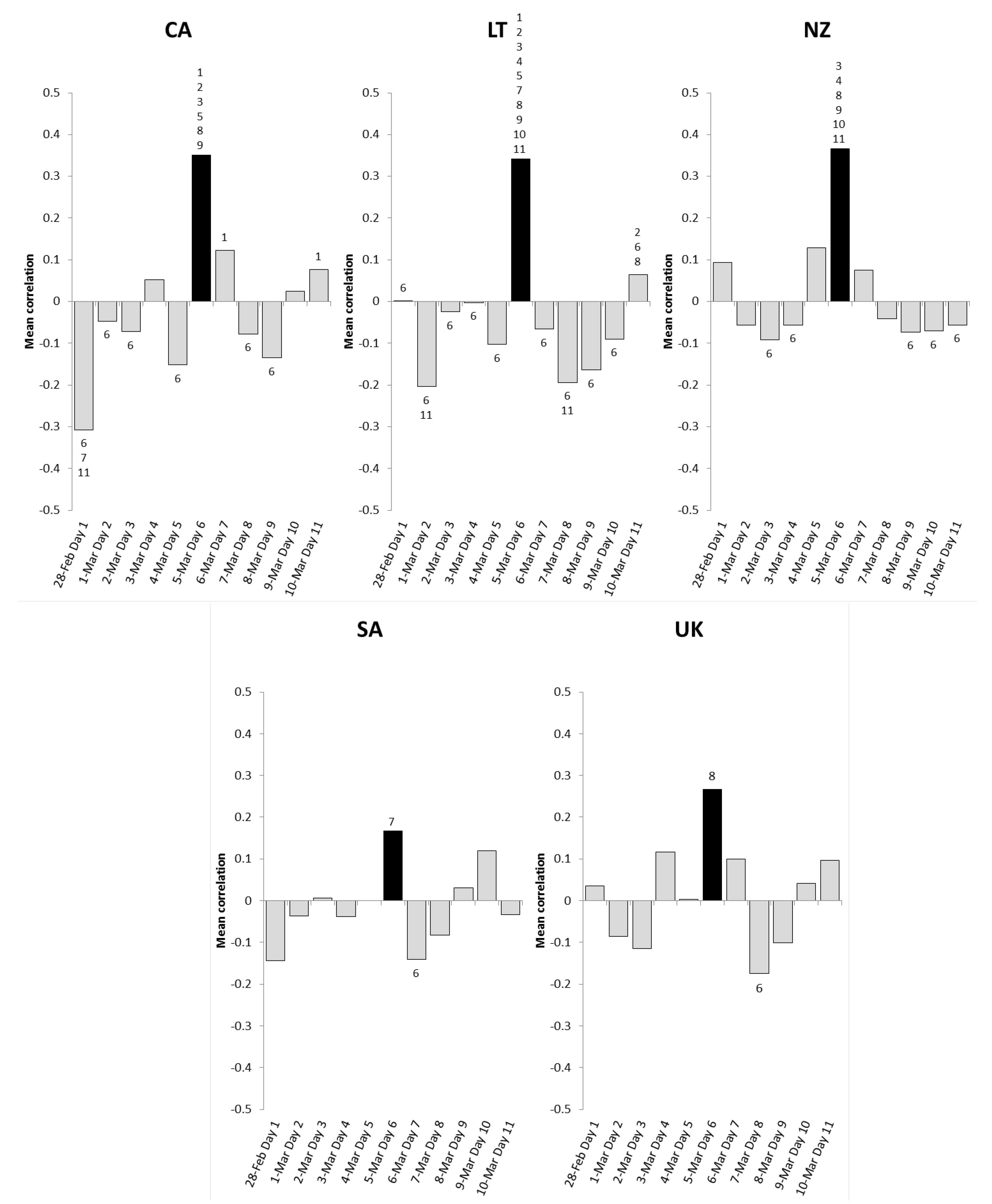
| Day | 28-February | 1-March | 2-March | 3-March | 4-March | 5-March | 6-March | 7-March | 8-March | 9-March | 10-March |
|---|---|---|---|---|---|---|---|---|---|---|---|
| 28-February | 0.26 | 0.24 | 0.36 | 0.16 | 0.66 *** | 0.43 * | 0.23 | 0.17 | 0.33 | 0.38 * | |
| 1-March | −0.26 | −0.03 | 0.1 | −0.11 | 0.40 * | 0.17 | −0.03 | −0.09 | 0.07 | 0.12 | |
| 2-March | −0.24 | 0.03 | 0.13 | −0.08 | 0.42 *** | 0.19 | −0.01 | −0.06 | 0.1 | 0.15 | |
| 3-March | −0.36 | −0.1 | −0.13 | −0.21 | 0.3 | 0.07 | −0.13 | −0.19 | −0.03 | 0.02 | |
| 4-March | −0.16 | 0.11 | 0.08 | 0.21 | 0.50 *** | 0.27 | 0.07 | 0.02 | 0.18 | 0.23 | |
| 5-March | −0.66 *** | −0.40 * | −0.42 *** | −0.3 | −0.50 *** | −0.23 | −0.43 * | −0.49 ** | −0.33 | −0.28 | |
| 6-March | −0.43 * | −0.17 | −0.19 | −0.07 | −0.27 | 0.23 | −0.2 | −0.26 | −0.1 | −0.05 | |
| 7-March | −0.23 | 0.03 | 0.01 | 0.13 | −0.07 | 0.43 * | 0.2 | −0.06 | 0.1 | 0.15 | |
| 8-March | −0.17 | 0.09 | 0.06 | 0.19 | −0.02 | 0.49 ** | 0.26 | 0.06 | 0.16 | 0.21 | |
| 9-March | −0.33 | −0.07 | −0.1 | 0.03 | −0.18 | 0.33 | 0.1 | −0.1 | −0.16 | 0.05 | |
| 10-March | −0.38 * | −0.12 | −0.15 | −0.02 | −0.23 | 0.28 | 0.05 | −0.15 | −0.21 | −0.05 |
| Day | 28-February | 1-March | 2-March | 3-March | 4-March | 5-March | 6-March | 7-March | 8-March | 9-March | 10-March |
|---|---|---|---|---|---|---|---|---|---|---|---|
| 28-February | −0.21 | −0.03 | 0 | −0.1 | 0.34 ** | −0.07 | −0.2 | −0.17 | −0.09 | 0.06 | |
| 1-March | 0.21 | 0.18 | 0.2 | 0.1 | 0.55 *** | 0.14 | 0.01 | 0.04 | 0.11 | 0.27 * | |
| 2-March | 0.03 | −0.18 | 0.02 | −0.08 | 0.37 *** | −0.04 | −0.17 | −0.14 | −0.06 | 0.09 | |
| 3-March | 0 | −0.2 | −0.02 | −0.1 | 0.35 *** | −0.06 | −0.19 | −0.16 | −0.09 | 0.07 | |
| 4-March | 0.1 | −0.1 | 0.08 | 0.1 | 0.45 ** | 0.04 | −0.09 | −0.06 | 0.01 | 0.17 | |
| 5-March | −0.34 ** | −0.55 *** | −0.37 *** | −0.35 *** | −0.45 ** | −0.41 ** | −0.54 *** | −0.51 *** | −0.43 *** | −0.28 * | |
| 6-March | 0.07 | −0.14 | 0.04 | 0.06 | −0.04 | 0.41 ** | −0.13 | −0.1 | −0.02 | 0.13 | |
| 7-March | 0.2 | −0.01 | 0.17 | 0.19 | 0.09 | 0.54 *** | 0.13 | 0.03 | 0.1 | 0.26 * | |
| 8-March | 0.17 | −0.04 | 0.14 | 0.16 | 0.06 | 0.51 *** | 0.1 | −0.03 | 0.07 | 0.23 | |
| 9-March | 0.09 | −0.11 | 0.06 | 0.09 | −0.01 | 0.43 *** | 0.02 | −0.1 | −0.07 | 0.16 | |
| 10-March | −0.06 | −0.27 * | −0.09 | −0.07 | −0.17 | 0.28 * | −0.13 | −0.26 * | −0.23 | −0.16 |
| Day | 28-February | 1-March | 2-March | 3-March | 4-March | 5-March | 6-March | 7-March | 8-March | 9-March | 10-March |
|---|---|---|---|---|---|---|---|---|---|---|---|
| 28-February | −0.15 | −0.19 | −0.15 | 0.03 | 0.27 | −0.02 | −0.13 | −0.17 | −0.17 | −0.15 | |
| 1-March | 0.15 | −0.04 | 0 | 0.18 | 0.42 | 0.13 | 0.02 | −0.02 | −0.02 | 0 | |
| 2-March | 0.19 | 0.04 | 0.04 | 0.22 | 0.46 ** | 0.17 | 0.05 | 0.02 | 0.02 | 0.04 | |
| 3-March | 0.15 | 0 | −0.04 | 0.18 | 0.42 ** | 0.13 | 0.02 | −0.02 | −0.02 | 0 | |
| 4-March | −0.03 | −0.18 | −0.22 | −0.18 | 0.24 | −0.05 | −0.17 | −0.2 | −0.2 | −0.18 | |
| 5-March | −0.27 | −0.42 | −0.46 ** | −0.42 ** | −0.24 | −0.29 | −0.41 * | −0.44 ** | −0.44 ** | −0.42 * | |
| 6-March | 0.02 | −0.13 | −0.17 | −0.13 | 0.05 | 0.29 | −0.12 | −0.15 | −0.15 | −0.13 | |
| 7-March | 0.13 | −0.02 | −0.05 | −0.02 | 0.17 | 0.41 * | 0.12 | −0.03 | −0.03 | −0.02 | |
| 8-March | 0.17 | 0.02 | −0.02 | 0.02 | 0.2 | 0.44 ** | 0.15 | 0.03 | 0 | 0.02 | |
| 9-March | 0.17 | 0.02 | −0.02 | 0.02 | 0.2 | 0.44 ** | 0.15 | 0.03 | 0 | 0.02 | |
| 10-March | 0.15 | 0 | −0.04 | 0 | 0.18 | 0.42 * | 0.13 | 0.02 | −0.02 | −0.02 |
| Day | 28-February | 1-March | 2-March | 3-March | 4-March | 5-March | 6-March | 7-March | 8-March | 9-March | 10-March |
|---|---|---|---|---|---|---|---|---|---|---|---|
| 28-February | 0.11 | 0.15 | 0.11 | 0.14 | 0.31 | 0 | 0.06 | 0.17 | 0.26 | 0.11 | |
| 1-March | −0.11 | 0.04 | 0 | 0.04 | 0.2 | −0.1 | −0.05 | 0.07 | 0.16 | 0 | |
| 2-March | −0.15 | −0.04 | −0.04 | −0.01 | 0.16 | −0.15 | −0.09 | 0.03 | 0.11 | −0.04 | |
| 3-March | −0.11 | 0 | 0.04 | 0.04 | 0.21 | −0.1 | −0.05 | 0.07 | 0.16 | 0.01 | |
| 4-March | −0.14 | −0.04 | 0.01 | −0.04 | 0.17 | −0.14 | −0.08 | 0.03 | 0.12 | −0.03 | |
| 5-March | −0.31 | −0.2 | −0.16 | −0.21 | −0.17 | −0.31 * | −0.25 | −0.14 | −0.05 | −0.2 | |
| 6-March | 0 | 0.1 | 0.15 | 0.1 | 0.14 | 0.31 * | 0.06 | 0.17 | 0.26 | 0.11 | |
| 7-March | −0.06 | 0.05 | 0.09 | 0.05 | 0.08 | 0.25 | −0.06 | 0.11 | 0.2 | 0.05 | |
| 8-March | −0.17 | −0.07 | −0.03 | −0.07 | −0.03 | 0.14 | −0.17 | −0.11 | 0.09 | −0.06 | |
| 9-March | −0.26 | −0.16 | −0.11 | −0.16 | −0.12 | 0.05 | −0.26 | −0.2 | −0.09 | −0.15 | |
| 10-March | −0.11 | 0 | 0.04 | −0.01 | 0.03 | 0.2 | −0.11 | −0.05 | 0.06 | 0.15 |
| Day | 28-February | 1-March | 2-March | 3-March | 4-March | 5-March | 6-March | 7-March | 8-March | 9-March | 10-March |
|---|---|---|---|---|---|---|---|---|---|---|---|
| 28-February | −0.12 | −0.15 | 0.08 | −0.03 | 0.23 | 0.07 | −0.21 | −0.14 | 0.01 | 0.06 | |
| 1-March | 0.12 | −0.03 | 0.2 | 0.09 | 0.35 | 0.18 | −0.09 | −0.02 | 0.13 | 0.18 | |
| 2-March | 0.15 | 0.03 | 0.23 | 0.12 | 0.38 | 0.22 | −0.06 | 0.01 | 0.16 | 0.21 | |
| 3-March | −0.08 | −0.2 | −0.23 | −0.11 | 0.15 | −0.02 | −0.29 | −0.22 | −0.08 | −0.02 | |
| 4-March | 0.03 | −0.09 | −0.12 | 0.11 | 0.26 | 0.1 | −0.18 | −0.1 | 0.04 | 0.09 | |
| 5-March | −0.23 | −0.35 | −0.38 | −0.15 | −0.26 | −0.17 | −0.44 * | −0.37 | −0.23 | −0.17 | |
| 6-March | −0.07 | −0.18 | −0.22 | 0.02 | −0.1 | 0.17 | −0.27 | −0.2 | −0.06 | 0 | |
| 7-March | 0.21 | 0.09 | 0.06 | 0.29 | 0.18 | 0.44 * | 0.27 | 0.07 | 0.22 | 0.27 | |
| 8-March | 0.14 | 0.02 | −0.01 | 0.22 | 0.1 | 0.37 | 0.2 | −0.07 | 0.14 | 0.2 | |
| 9-March | −0.01 | −0.13 | −0.16 | 0.08 | −0.04 | 0.23 | 0.06 | −0.22 | −0.14 | 0.06 | |
| 10-March | −0.06 | −0.18 | −0.21 | 0.02 | −0.09 | 0.17 | 0 | −0.27 | −0.2 | −0.06 |
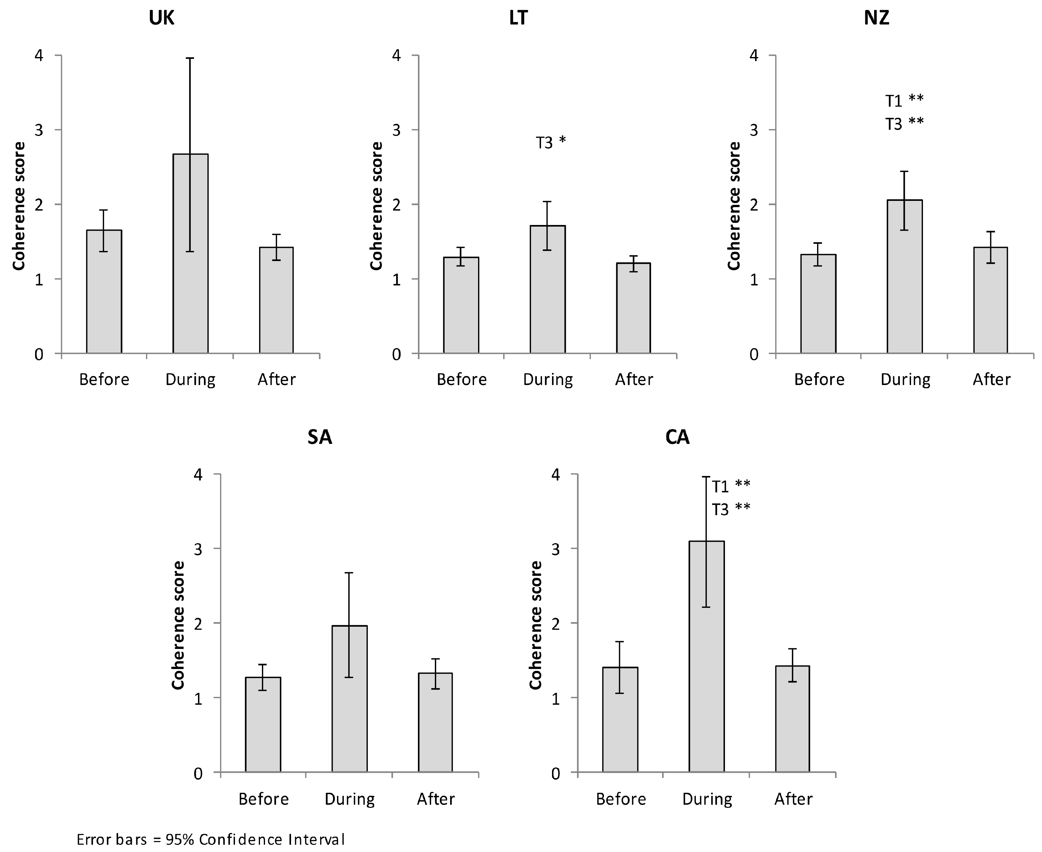
| Pairwise Comparisons b | ||||||||||||||
|---|---|---|---|---|---|---|---|---|---|---|---|---|---|---|
| Group | N | Mean | Lower 95% CI | Upper 95% CI | df | Mean Square | F | p< | p< 1 vs. 2 | p< 1 vs. 3 | p< 2 vs. 3 | |||
| UK | 1 Before | 9 | 1.65 | 1.38 | 1.92 | 1.05 a | 7.49 | 4.34 | ns | 0.35 | - | - | - | |
| 2 During | 9 | 2.67 | 1.37 | 3.96 | ||||||||||
| 3 After | 9 | 1.43 | 1.26 | 1.60 | ||||||||||
| LT | 1 Before | 19 | 1.30 | 1.17 | 1.42 | 1.196 a | 2.23 | 6.65 | 0.05 | 0.27 | ns | ns | 0.05 | |
| 2 During | 19 | 1.70 | 1.38 | 2.03 | ||||||||||
| 3 After | 19 | 1.21 | 1.10 | 1.32 | ||||||||||
| NZ | 1 Before | 19 | 1.33 | 1.18 | 1.48 | 1.389 a | 4.25 | 13.30 | 0.001 | 0.43 | 0.01 | ns | 0.01 | |
| 2 During | 19 | 2.05 | 1.65 | 2.45 | ||||||||||
| 3 After | 19 | 1.42 | 1.21 | 1.63 | ||||||||||
| SA | 1 Before | 11 | 1.27 | 1.10 | 1.45 | 1.097 a | 3.02 | 4.32 | ns | 0.30 | - | - | - | |
| 2 During | 11 | 1.97 | 1.27 | 2.67 | ||||||||||
| 3 After | 11 | 1.32 | 1.12 | 1.53 | ||||||||||
| CA | 1 Before | 11 | 1.40 | 1.05 | 1.76 | 1.086 a | 18.85 | 21.52 | 0.001 | 0.68 | 0.01 | ns | 0.01 | |
| 2 During | 11 | 3.09 | 2.21 | 3.96 | ||||||||||
| 3 After | 11 | 1.43 | 1.21 | 1.65 | ||||||||||
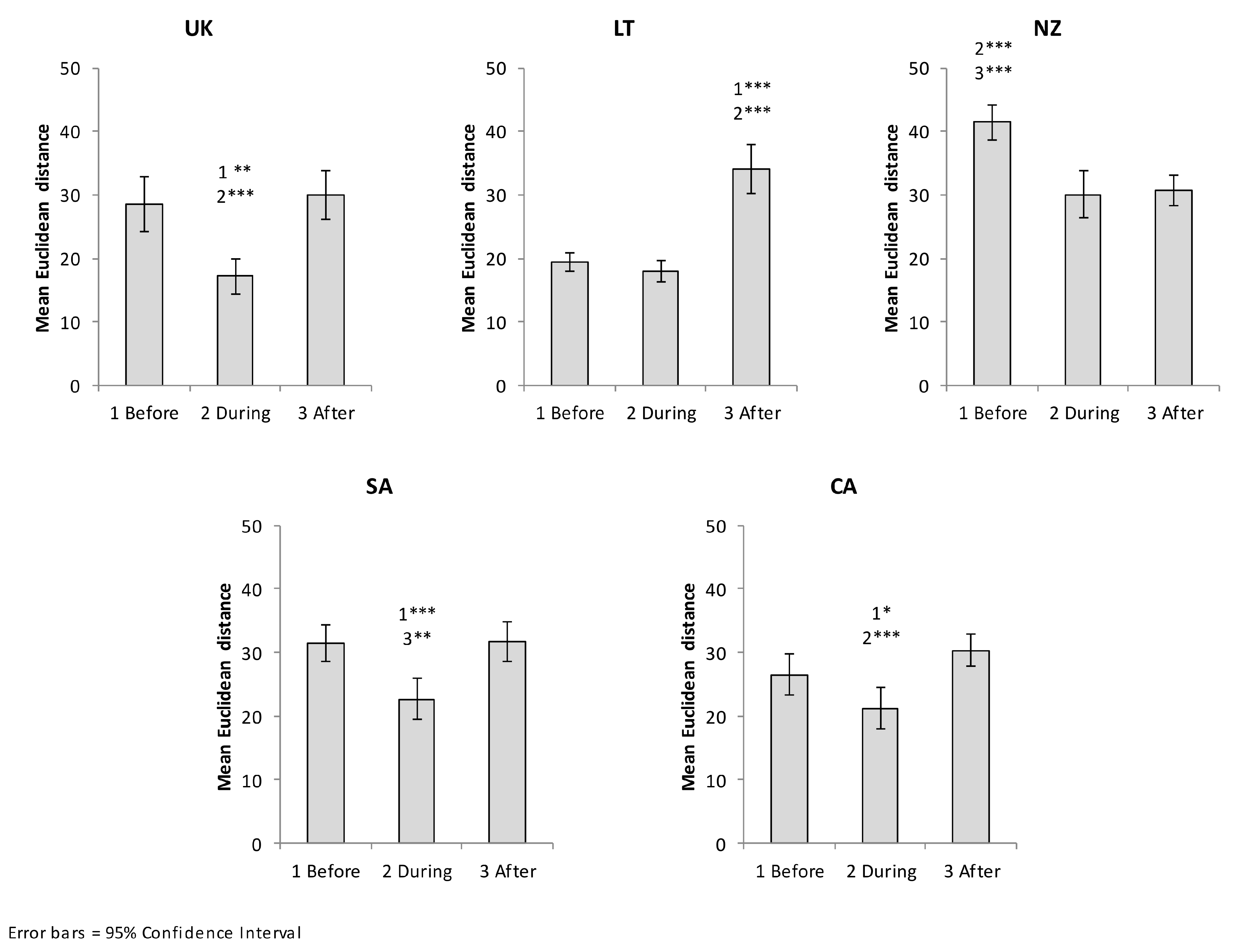
| Pairwise Comparisons b | ||||||||||||||
|---|---|---|---|---|---|---|---|---|---|---|---|---|---|---|
| Group | N | Mean | Lower 95% CI | Upper 95% CI | df | Mean Square | F | p< | p< 1 vs. 2 | p< 1 vs. 3 | p< 2 vs. 3 | |||
| UK | 1 Before | 8 | 28.64 | 24.38 | 32.90 | 2 | 390.00 | 16.73 | 0.001 | 0.71 | 0.01 | ns. | 0.001 | |
| 2 During | 8 | 17.28 | 14.54 | 20.02 | ||||||||||
| 3 After | 8 | 29.99 | 26.17 | 33.81 | ||||||||||
| LT | 1 Before | 16 | 19.51 | 18.12 | 20.90 | 1.2 a | 2128.96 | 52.90 | 0.001 | 0.78 | ns. | 0.001 | 0.001 | |
| 2 During | 16 | 18.05 | 16.31 | 19.80 | ||||||||||
| 3 After | 16 | 34.21 | 30.37 | 38.05 | ||||||||||
| NZ | 1 Before | 19 | 41.49 | 38.73 | 44.26 | 2 | 777.36 | 18.34 | 0.001 | 0.51 | 0.001 | 0.001 | ns | |
| 2 During | 19 | 30.09 | 26.39 | 33.79 | ||||||||||
| 3 After | 19 | 30.78 | 28.40 | 33.15 | ||||||||||
| SA | 1 Before | 11 | 31.53 | 28.63 | 34.42 | 2 | 294.63 | 16.48 | 0.001 | 0.62 | 0.001 | ns | 0.01 | |
| 2 During | 11 | 22.67 | 19.36 | 25.98 | ||||||||||
| 3 After | 11 | 31.74 | 28.55 | 34.93 | ||||||||||
| CA | 1 Before | 11 | 26.52 | 23.25 | 29.79 | 2 | 233.94 | 18.38 | 0.001 | 0.65 | 0.05 | ns | 0.001 | |
| 2 During | 11 | 21.21 | 17.98 | 24.43 | ||||||||||
| 3 After | 11 | 30.39 | 27.87 | 32.91 | ||||||||||
Publisher’s Note: MDPI stays neutral with regard to jurisdictional claims in published maps and institutional affiliations. |
© 2021 by the authors. Licensee MDPI, Basel, Switzerland. This article is an open access article distributed under the terms and conditions of the Creative Commons Attribution (CC BY) license (http://creativecommons.org/licenses/by/4.0/).
Share and Cite
Timofejeva, I.; McCraty, R.; Atkinson, M.; Alabdulgader, A.A.; Vainoras, A.; Landauskas, M.; Šiaučiūnaitė, V.; Ragulskis, M. Global Study of Human Heart Rhythm Synchronization with the Earth’s Time Varying Magnetic Field. Appl. Sci. 2021, 11, 2935. https://doi.org/10.3390/app11072935
Timofejeva I, McCraty R, Atkinson M, Alabdulgader AA, Vainoras A, Landauskas M, Šiaučiūnaitė V, Ragulskis M. Global Study of Human Heart Rhythm Synchronization with the Earth’s Time Varying Magnetic Field. Applied Sciences. 2021; 11(7):2935. https://doi.org/10.3390/app11072935
Chicago/Turabian StyleTimofejeva, Inga, Rollin McCraty, Mike Atkinson, Abdullah A. Alabdulgader, Alfonsas Vainoras, Mantas Landauskas, Vaiva Šiaučiūnaitė, and Minvydas Ragulskis. 2021. "Global Study of Human Heart Rhythm Synchronization with the Earth’s Time Varying Magnetic Field" Applied Sciences 11, no. 7: 2935. https://doi.org/10.3390/app11072935