Impact of Grounding Modeling on Lightning-Induced Voltages Evaluation in Distribution Lines

Abstract

Lightning-induced voltages are one of the main causes of shutdown in distribution lines. In this work, attention is focused on the effects of wideband modeling of electric grounding in the overvoltage calculation along insulator strings due to indirect lightning strikes. This study is done directly in the time-domain with the grounding being represented with an equivalent circuit accounting for its dynamics. Results show that the adoption of commonly adopted simplified grounding models, such as low-frequency resistance, may lead to an underestimation of the overvoltage. According to the results, differences in the order of 25% can be found in some studied cases.

1. Introduction

Transmission and Distribution Systems are highly affected and damaged by direct and indirect lightning events. Direct events occur when lightning directly strikes the line; such events are hazardous but rare and are typically studied and analyzed in Transmission System (TS). On the other hand, indirect events occur when lightning strikes the ground in the proximity of a power system; these events are much more frequent with respect to direct ones, but the overall voltage induced in the power system is usually much lower. For this reason, indirect events are not of interest for TS since the induced voltages are generally lower than the line Critical FlashOver voltage (CFO), but they are vital when dealing with Distribution Systems (DS), which are characterized by a low CFO.

Most works address lightning-induced voltages in DS model electric grounding as a constant value resistance $R_{LF}$ [1,2,3,4,5,6,7,8,9,10,11,12,13,14,15,16]. This parameter is associated with a low-frequency behavior, i.e., disregarding its electromagnetic dynamic. Therefore, this low-frequency grounding resistance cannot reproduce the reactive (inductive and capacitive) and electromagnetic wave propagation effects (attenuation and distortion), prominent in the high-frequency range related to the voltage and current wavefronts. Additionally, the determination of overvoltage on TS, due to direct lightning, is highly sensible on the electromagnetic modeling of the electrical grounding [17].

Given the above, this work presents an evaluation of the impact of grounding modeling on lightning-induced voltage. Thus, the main original contribution of this paper is to include, in the time domain type simulations, an equivalent electric circuit that reproduces the complete frequency response of grounding, with full inclusion of the aforementioned effects. The Hybrid Electromagnetic Model (HEM) is used to determine the wideband grounding frequency response $Z\left(\omega \right)$[18,19]. To implement the $Z\left(\omega \right)$ in silico, the Vector Fitting (VF) technique is applied to generate an equivalent electric circuit that is easily inserted in EMT-type software [20,21]. In the following, the grounding circuit will be implemented in the software developed in [22]. In this paper, as commonly proposed in the IEEE Standard [5], the coupling between the tower and the lightning channel and the coupling between the lightning channel and the grounding electrodes are neglected.

The results illustrate that the induced voltages, considering the grounding modeled via $R_{LF}$ are quite different from those results using $Z\left(\omega \right)$, with perceptual differences reaching values of around 25%. It is noticeable that the differences increase with the soil resistivity and with the point of occurrence of the lightning (lightning striking closer to the DS increase the perceptual differences) for both first and subsequent return strokes. The paper is organized as follows: Section 2, Section 3 and Section 4 show the lightning field-to-line coupling problem equations, the tower and the grounding modeling, respectively; while Section 5 and Section 6 present the test cases and the results. Section 7 is dedicated to the conclusions.

2. Induced-Lightning Modeling

The lightning-induced voltages occurring in a DS are here evaluated, recalling the procedure presented in [22,23]. This procedure is usually divided into two steps: (i) the ElectroMagnetic (EM) fields computation and (ii) the field-to-line coupling.

2.1. EM Fields Computation

The EM fields are computed analytically considering the approach proposed in [24] and validated in [25]. The method requires as input the knowledge of the channel-base current, the return stroke height and the return stroke velocity. It can be applied both to perfect electric conductor ground and soil characterized by a finite conductivity. The only assumption required is the Transmission Line model for the attenuation of the current along the channel. The main advantage of this approach consists of the possibility of dealing with analytical formulas, which guarantee a fast solution and a low computational effort.

2.2. Field-to-Line Coupling

The field-to-line coupling computation is obtained considering the well-known Agrawal model [26], which is here presented in its extended version taking into account the presence of a finite-conducting ground and a multi-conductor line.

$$\left\{\begin{array}{l}\frac{\partial V_i^s}{\partial x}\left(x,t\right)+\sum _{j=1}^M{L}_{ij}\frac{\partial I_j}{\partial t}\left(x,t\right)+V_i^g(x,t)=E_{inc,x,i}^{}\left(x,t\right)\hfill \\ \frac{\partial I_i}{\partial x}\left(x,t\right)+\sum _{j=1}^M{C}_{ij}\frac{\partial V_j^s}{\partial t}\left(x,t\right)=0\end{array}\right.$$

(1)

with

$$V_i^g\left(x,t\right)=\underset{0}{\overset{t}{\int }}{\xi }_g^i\left(t-s\right)\frac{\partial I_i}{\partial s}\left(x,s\right)ds$$

(2)

where $V_i^s\left(x,t\right)$, $I_i\left(x,t\right)$ and $E_{inc,x,i}^{}\left(x,t\right)$ are the scattered voltage, the current and the tangential component of the exciting electric field (computed in the previous subsection) on the ith conductor at distance x from the beginning of the line. As expressed in Equation (1), the knowledge of the inductance and capacitance matrices (L and C) is required. Please note that ${\xi }_i^g$ is the time-domain expression for the ground impedance [27].

The total voltage occurring on the i-th conductor at the point x can be then expressed as the sum of the scattered voltage and the incident voltage, whose value depends on the vertical electric field (computed in the previous subsection).

The proposed methodology is adapted to an EMT-type software (in this framework Simulink-Simscape is used), through the finite-difference time-domain (FDTD) technique. In this case, a second-order scheme is adopted with $dt=10$ ns and $dx=9$ m, which satisfies the well-known Courant stability condition. Further details can be found in [22].

3. Tower Modeling

The modeling of the tower is usually neglected in lightning-induced voltages studies. However, in this framework, the tower is included in the model according to [28,29] and is modeled as a lossless transmission line, whose characteristic impedance is:

$$Z_c=60\left[ln\left(\sqrt{2}\frac{2h}{r}\right)-1+\frac{r}{4h}+{\left(\frac{r}{4h}\right)}^2\right]$$

(3)

h being the tower height and r the tower radius.

4. Electrical Grounding Modeling

In this paper, the grounding transient behavior is modeled by HEM [18,19]. This model is an electromagnetic computational method developed for the numerical solution of lightning problems and, according to CIGRÉ [30], it is classified as a hybrid electromagnetic-circuit approach. The main motivations for using HEM are as follows: (i) it is accurate and flexible, i.e., it can be used in different types of grounding configuration; (ii) its results have been extensively validated experimentally, such as measurements in TS [18,19], horizontal electrodes [18,31], vertical rods [31,32], and typical substation grounding grids [33] and (iii) it is faster than traditional full-wave methods (without losing accuracy). It is worth mentioning that the usage of HEM has increased significantly recently [30,34,35].

Basically, HEM consists of subdividing the actual system (in this case, electrical grounding) into N small conductive cylindrical segments and, for each segment, the electromagnetic theory is applied. After that, by using the circuit theory, it is possible to obtain a matrix system that computes the wideband response of the electrical grounding. For the sake of clarity, we present a brief overview of HEM below. More details about HEM are described in [18,19].

It is worth commenting on the fact that HEM corresponds to an electromagnetic model developed in the frequency domain. Thus, it is necessary first to determine the frequency spectrum (depending on the phenomenon of interest). After that, the electrical grounding is divided into N segments, where the length of each segment is equal to 10 times its radius (thin wire approximation). A discussion about segmentation length is presented in [36].

Each segment is considered a source of two currents, one longitudinal that flows along the electrode ($I_L$) and another transversal that flows from the electrode to the surrounding soil ($I_T$). It is worth noting that $I_L$ generates a non-conservative electric field and $I_T$ a conservative one. With the aid of the magnetic vector and electric scalar potentials, both voltage drops ($\Delta V$) and electric potentials (V) in each pair of segments (transmitter and receiver) are determined. Additionally, double integral equations are established for $\Delta V$ and V. These integrals depend on the frequency, geometry, soil parameters and $I_T$ and $I_L$ distributions. However, the distributions of $I_T$ and $I_L$ are not known and are integrands of the integrals. From this point on, the Method of Moments (MoM) is applied to solve these integral equations [37]. The effect of the air-soil interface is included using the method of images, similar to [38,39].

The $I_T$ and $I_L$ distributions considered in this paper are of the piecewise-constant function type [18,19]. MoM makes it possible to transform integral equations into algebraic ones, the solution of which allows determining all the quantities of interest (in the frequency domain), such as $I_T$, $I_L$,$\Delta V$ and V distributions; transverse (capacitive and conductive couplings) and longitudinal (resistive and inductive couplings) impedances (self and mutual); electromagnetic field; harmonic grounding impedance ($Z\left(\omega \right)$); low-frequency grounding resistance ($R_{LF}$), etc.

Also, it has been documented in the literature, over almost one hundred years [40], that the soil is a dispersive medium, i.e., the response is not instantaneous. Several researchers have presented a numerical solution to consider this dispersivity in the frequency domain, such as [31,40,41,42,43,44,45,46,47,48,49]. According to [50], for the values of conductivity considered in this paper, the frequency-dependent soil electric parameters can be neglected in the computation of the EM fields that illuminate the line. On the other hand, according to [17], the impact of considering the frequency-dependence of the soil in the grounding modeling generates sensible differences. Thus, in this paper, the frequency-dependence of the soil parameters is considered in the grounding modeling. Use is made by the formulations proposed in [31], since a CIGRE Brochure has suggested them [51]. Equations (4) and (5) illustrate the formulation.

$$\sigma \left(f\right)={\sigma }_0+{\sigma }_{0}h\left({\sigma }_0\right){\left(f\times {10}^{-6}\right)}^{\gamma }$$

(4)

$${ϵ}_r\left(f\right)={ϵ}_{r\infty }+\frac{tan(\pi \gamma /2)\times {10}^{-3}}{2\pi {ϵ}_0{\left({10}^6\right)}^{\gamma }}{\sigma }_{0}h\left({\sigma }_0\right)f^{(\gamma -1)}$$

(5)

where $\sigma \left(f\right)$ is the frequency-dependent soil conductivity (in mS/m), ${\sigma }_0$ is the low-frequency soil conductivity (in mS/m), ${ϵ}_r\left(f\right)$ is the frequency-dependent soil permittivity and ${ϵ}_0$ is the vacuum permittivity. To obtain mean results (more details about it in [31]), one should use $h\left({\sigma }_0\right)=1.26{\sigma }_0^{-0.73}$, $\gamma =0.54$ and ${ϵ}_{r\infty }=12$.

As specified before, the calculation of induced voltages is performed directly in the time domain; however, $Z\left(\omega \right)$ is a frequency domain quantity. Thus, the well-known Vector Fitting (VF) approach is used for fitting the calculated frequency domain grounding response with rational function approximations [20]. The passivity is enforced by perturbation [21].

Finally, based on the obtained rational function, it is possible to synthesize an electric network that can be promptly included in the time-domain simulation. It is important to note that this electric circuit generates the same frequency response as the harmonic grounding impedance provided by HEM. Thus, it includes reactive and electromagnetic wave propagation effects.

5. Test Cases

This section presents the test cases related to the comparison between two different grounding modeling, i.e., the low-frequency grounding resistance ($R_{LF}$) and the harmonic grounding impedance ($Z\left(\omega \right)$).

Let us consider a 1.2 km matched three-phase DS (Figure 1). The three-phase conductors’ heights are 10, 11 and 12 m, respectively, while the shield wire height is 14 m. The horizontal distance between each conductor and the shield wire is 2.4 m. The conductors’ diameter is 1.83 cm, while the shield wire diameter is 0.72 cm.

The span between each tower is 50 m. To consider the influence of the adjacent towers, a total of five towers are modeled in detail, because the towers in longer distance have little impact on the overvoltage. According to [52], for lightning-related phenomena adjacent towers place a moderate influence. Each tower is 14 m high and with a base diameter of 0.5 m. According to Equation (3), a value of $Z_c=244.17\Omega$ is considered. The propagation velocity along the tower is considered to be $0.8c$ [53,54]. Moreover, the insulators are modeled taking into account their parasitic capacitance. The value of parasitic capacitance of each insulator is 7.68 nF, and they were calculated considering the information in [55,56,57].

Each tower is grounded with a grounding system as shown in Figure 2. This is a typical configuration for grounding distribution networks in the State of Minas Gerais, Brazil. It consists of three vertical rods 2.5 m long interconnected by a horizontal galvanized steel cable 6 m long. The vertical rods are copper-plated steel, with a diameter of 15 mm.

The equivalent circuit of the system composed of a three-phase distribution line, tower and grounding system is shown in Figure 3.

Two cases for the soil parameters will be considered. The soil conductivity and permittivity will be frequency-dependent according to [31], where ${\sigma }_0=$ 10 mS/m and 1 mS/m, respectively. These cases correspond to two different grounding harmonic responses according to the grounding modeling proposed in Section 4. Figure 4 and Figure 5 show $Z\left(\omega \right)$ and $R_{LF}$ of the two considered cases. Based on the behaviors described in these figures, it is possible to verify that: (i) grounding can only be represented by $R_{LF}$ in the low-frequency range, where $Z\left(\omega \right)$ tends to $R_{LF}$; (ii) the limit frequency of the low-frequency range increases with a reduction in conductivity; (iii) in the intermediate-frequency range there is a predominance of capacitive behavior of the grounding, verified by the decrease of $Z\left(\omega \right)$ in relation to the $R_{LF}$; (iv) the limit frequency of the intermediate-frequency range also increases with the reduction in conductivity and (v) only in the high-frequency range inductive effect is predominant, mainly for higher conductivity values. Thus, the response of the system under study (DS and grounding) will be a direct function of the frequency spectrum of the electromagnetic signal that requests it. As a consequence, it is expected that the overvoltages in the insulator string are sensitive to grounding modeling.

When we consider a grounding model described by $R_{LF}$, the implementation in the EMT-type software is trivial, while when we consider the harmonic grounding impedance, it is possible to obtain the synthesis of the electric circuit to be implemented in the EMT-type software by using the approach presented in Section 4.

The general layout of the circuit obtained from the Vector fitting approach is described in Figure 6, while the values of the passive circuit are proposed in

Table 1. Elements of Real Poles of the grounding circuit. $\sigma$ = 10 mS/m.

i	Resistance [$\mathbf{\Omega }$]	Inductance [mH]	Capacitance [$\mathsf{\mu }$F]
0	3.33 × ${10}^{15}$	-	3.00 × ${10}^{-10}$
1	−4.23 × ${10}^3$	−1.44 × ${10}^4$	-
2	−3.12 × ${10}^3$	−2.25 × ${10}^3$	-
3	−1.83 × ${10}^3$	−3.96 × ${10}^2$	-
4	−1.03 × ${10}^3$	−70.87	-
5	−5.81 × ${10}^2$	−12.83	-
6	−3.23 × ${10}^2$	−2.33	-
7	−1.75 × ${10}^2$	−0.41	-
8	−83.82	−6.38 × ${10}^2$	-
9	−5.40 × ${10}^3$	−9.35 × ${10}^{-4}$	-
10	11.77	3.09 × ${10}^{-4}$	-
11	−7.65	−5.21 × ${10}^{-5}$	-
12	6.21	1.32 × ${10}^{-5}$	-

and

Table 2. Elements of Complex Poles of the grounding circuit. $\sigma$ = 10 mS/m.

i	Resistance [$\mathbf{\Omega }$]	Inductance [mH]	Capacitance [$\mathsf{\mu }$F]	Conductance [mS]
1	−2.35	1.25 × ${10}^{-3}$	6.70 × ${10}^{-3}$	1.26 × ${10}^2$

for $\sigma =$ 10 mS/m and in

Table 3. Elements of Real Poles of the grounding circuit. $\sigma$ = 1 mS/m.

i	Resistance [$\mathbf{\Omega }$]	Inductance [mH]	Capacitance [$\mathsf{\mu }$F]
0	3.33 × ${10}^{15}$	-	3.00 × ${10}^{-10}$
1	−6.35 × ${10}^3$	−5.67 × ${10}^3$	-
2	−8.44 × ${10}^3$	−1.19 × ${10}^3$	-
3	−1.30 × ${10}^3$	−3.66 × ${10}^1$	-
4	−2.75 × ${10}^3$	−1.74 × ${10}^1$	-
5	−2.78 × ${10}^2$	−4.23 × ${10}^{-1}$	-
6	−8.96 × ${10}^2$	−3.39 × ${10}^{-1}$	-
7	−3.13 × ${10}^1$	−1.98 × ${10}^{-3}$	-
8	1.77 × ${10}^{-5}$	5.00 × ${10}^{-5}$	-

and

Table 4. Elements of Complex Poles of the grounding circuit. $\sigma$ = 1 mS/m.

i	Resistance [$\mathbf{\Omega }$]	Inductance [mH]	Capacitance [$\mathsf{\mu }$F]	Conductance [mS]
1	1.58 × ${10}^1$	2.28 × ${10}^{-3}$	1.89 × ${10}^{-3}$	5.18
2	2.28 × ${10}^3$	1.11 × ${10}^{-2}$	2.34 × ${10}^{-6}$	−0.42
3	3.35 × ${10}^2$	−9.12 × ${10}^{-3}$	−2.16 × ${10}^{-5}$	−1.12

for $\sigma =$ 1 mS/m. It is worth mentioning that these equivalent circuits are mathematical models that have a frequency response very close to $Z\left(\omega \right)$, but their electrical parameters do not have physical consistency, it is also important mentioning that although some elements may have negative values, the circuit is passive in overall. Hence the existence of negative values for resistance, inductance and capacitance in Table 1, Table 2, Table 3 and Table 4 do not mean that the circuit is not passive. The i-index appearing in Table 1, Table 2, Table 3 and Table 4 refers to the electrical branch.

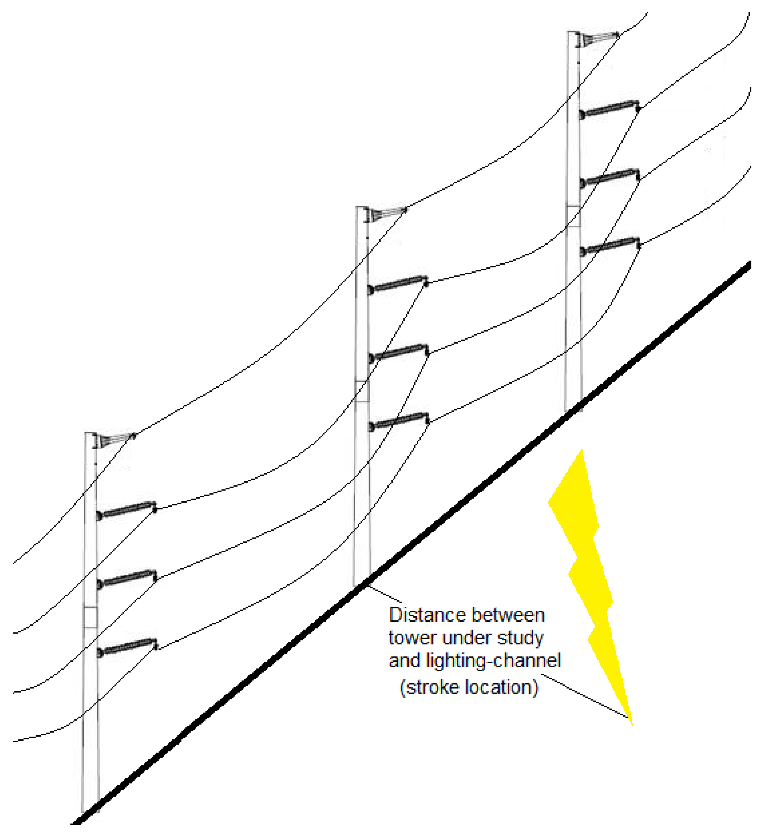
To compare the grounding modeling, 12 different tests have been implemented (

Table 5. Test details.

Test	$\mathit{\sigma }$ [S/m]	Stroke Distance [m]	Stroke Type
T1	0.01	60	First
T2	0.01	200	First
T3	0.01	2000	First
T4	0.001	60	First
T5	0.001	200	First
T6	0.001	2000	First
T7	0.01	60	Subsequent
T8	0.01	200	Subsequent
T9	0.01	2000	Subsequent
T10	0.001	60	Subsequent
T11	0.001	200	Subsequent
T12	0.001	2000	Subsequent

), each one differing for the soil conductivity, stroke location and stroke type (first or subsequent). The stroke location is always placed in front of the middle of the line, Figure 7 illustrates the distance between the lightning-channel and the tower under study. It is important to highlight that if the closest point of the DS to the stroke location is in the mid-span, it would, naturally, change the maximum overvoltage but not the perceptual differences between the approaches. The lightning return stroke channel is characterized by a height of 8 km and a speed equal to one-half the speed of light in a vacuum. The channel-base current is modeled as a sum of two Heidler’s functions as in Equation (6), with parameters reported in

Table 6. Heidler’s current parameters.

Parameter	First	Subsequent
$I_{01}$ [kA]	28.0	10.7
${\tau }_{11}$ [$\mathsf{\mu }$s]	1.8	0.22
${\tau }_{12}$ [$\mathsf{\mu }$s]	95.0	2.5
$n_1$	2	2
$I_{02}$ [kA]	-	6.5
${\tau }_{21}$ [$\mathsf{\mu }$s]	-	2.1
${\tau }_{22}$ [$\mathsf{\mu }$s]	-	230.0
$n_2$	-	2

. The representation of the channel-base current is proposed in Figure 8 and Figure 9.

$$I_0\left(t\right)=\frac{I_{01}}{{{\eta }_1}_{}}\frac{{\left(\frac{t}{{\tau }_{11}}\right)}^{n_1}}{1+{\left(\frac{t}{{\tau }_{11}}\right)}^{n_1}}{e}^{-\frac{t}{{\tau }_{12}}}+\frac{I_{02}}{{{\eta }_2}_{}}\frac{{\left(\frac{t}{{\tau }_{21}}\right)}^{n_2}}{1+{\left(\frac{t}{{\tau }_{21}}\right)}^{n_2}}{e}^{-\frac{t}{{\tau }_{22}}}$$

(6)

being

$${\eta }_i=exp\left(-\frac{{\tau }_{i1}}{{\tau }_{i2}}{\left(n_i\frac{{\tau }_{i2}}{{\tau }_{i1}}\right)}^{\frac{1}{n_i}}\right)$$

(7)

6. Results

In this section, the results for the test cases of Table 5 are presented, showing the voltage across the phase B insulator string ($V_{insulator}$ in Figure 3) and the voltage difference occurring on the grounding system ($V_{grounding}$ in Figure 3).

Figure 10, Figure 11, Figure 12, Figure 13, Figure 14 and Figure 15 show the results for tests T1–T6, corresponding to a typical first stroke. The main differences in terms of voltage across the insulator can be observed considering a low soil conductivity (Figure 13, Figure 14 and Figure 15) and near stroke locations (60 m). This is extremely important because the closer the stroke location, the higher (and the more dangerous) the induced voltage. For example, let us consider Test T4 (Figure 13). If we use the low-frequency grounding resistance ($R_{LF}$) as grounding model, the maximum induced voltage across the insulator string is 115.12 kV, while if we consider the harmonic grounding impedance ($Z\left(\omega \right)$), which represents in a better way the reality, the voltage is 119.40 kV. This shows how the difference in the modeling could lead to either a fault or not across the insulator strings.

On the other hand, when the harmonic grounding impedance model presents a voltage across the insulator higher with respect to the $R_{LF}$ case, the voltage on the grounding system is lower. This can be explained as follows: let us consider Figure 3; the voltage difference occurring on the insulator string is

$$V_{insulator}=V_{conductor}-V_{sw}$$

(8)

It is reasonable to assume that the voltage on the conductor does not change in a meaningful way. Considering the two different approaches (based on grounding system modeling), the only difference is the current flowing in the shield wire conductor causing a different coupling with the phase conductor. Even if not negligible, the coupling between conductors does not represent the dominant aspect in the lightning-induced voltages (which is the electric field illuminating the conductor). Consequently, $V_{insulator}+V_{sw}$ is almost constant. The shield wire voltage is:

$$V_{sw}=V_{tower}+V_{grounding}$$

(9)

with the same current, $V_{tower}$ is constant in the two cases but $V_{grounding}$ varies because the impedance varies according to Figure 4 and Figure 5 for $\sigma =$ 10 mS/m and 1 mS/m, respectively. Let us consider the most critical case, i.e., $\sigma =1$ mS/m: from Figure 5 it is clear that for each considered frequency $Z\left(\omega \right)<R_{LF}$, thus with the same current the voltage on the grounding system is lower if we consider the harmonic impedance $Z\left(\omega \right)$ and consequently also $V_{sw}$ is lower. Since $V_{insulator}+V_{sw}=constant$, if $V_{sw}$ decreases, $V_{insulator}$ increases. This aspect is confirmed in Tests T4-T5-T6, T10-T11-T12.

The results for subsequent strokes can be observed in Figure 16, Figure 17, Figure 18, Figure 19, Figure 20 and Figure 21. The results are in agreement with the previous ones, confirming a significant increase of the maximum voltage if the equivalent circuit ($Z\left(\omega \right)$) is taken into account, especially if the soil conductivity is low. Moreover, the percentage increase considering the harmonic grounding impedance with respect to the low-frequency resistance is much more significant with respect to the first stroke case considering $\sigma =1$ mS/m. It is expected since the subsequent strokes are faster. Thus, it has a higher frequency spectrum (the region where there are the highest differences between $R_{LF}$ and $Z\left(\omega \right)$). Additionally, it is important to highlight that after a while, both overvoltages, considering $R_{LF}$ and $Z\left(\omega \right)$, tend to the same value (first and subsequent strokes). For instance, if we consider the T10 and use the $R_{LF}$ as grounding model, the maximum induced voltage across the insulator string is 66 kV, while if we consider the $Z\left(\omega \right)$, the voltage is 81 kV. This shows how the modeling difference could lead to either a fault or not across the insulator strings, especially for subsequent strokes.

Finally,

Table 7. Maximum voltage across the insulator. Percentage increase considering the harmonic grounding impedance ($Z\left(\omega \right)$) with respect to the low-frequency grounding resistance ($R_{LF}$).

Test	Voltage Insulator Increase [%]
T1	0.56
T2	0.26
T3	0.08
T4	3.50
T5	4.95
T6	6.76
T7	1.73
T8	1.80
T9	1.26
T10	22.54
T11	11.31
T12	23.06

shows the percentage increase in the maximum voltage across the phase B insulator considering the harmonic grounding impedance ($Z\left(\omega \right)$) with respect to the low-frequency grounding resistance ($R_{LF}$). According to the previous considerations, the differences are almost negligible if the soil conductivity is high (tests T1–T3 and T7–T9), but they become consistent when the soil conductivity decreases (tests T4–T6 and T10–T12). This behavior is more evident for close stroke location (test T4 and T10).

7. Conclusions

Lightning induced-voltages are usually computed considering only the low-frequency grounding resistance when one considers the grounding system of the distribution tower. This work presented the impact of two different models for the grounding system of distribution line towers on the lightning-induced voltage on the phase insulators computation. The comparison between the low-frequency grounding resistance ($R_{LF}$) and the equivalent circuit corresponding to the wideband grounding frequency response ($Z\left(\omega \right)$) shows that considering only $R_{LF}$ may lead to non-negligible underestimation of the maximum induced voltage. This aspect is more evident for subsequent strokes in the case of close stroke locations and low soil conductivities, which represents, by the way, one of the configurations when the lightning-induced voltages on a distribution line are high and potentially dangerous. On the other hand, for high soil conductivity, the differences between the two models are negligible. Future work will extend this analysis to the evaluation of a distribution line lightning performance to check whether this trend is also confirmed when dealing with statistical calculations. Additionally, in future works it is expected to include the coupling between the lightning channel and the grounding electrodes, similarly, as presented in [58].

References

1. Cooray, V.; Scuka, V. Lightning-induced overvoltages in power lines: Validity of various approximations made in overvoltage calculations. IEEE Trans. Electr. Compatib. 1998, 40, 355–363. [Google Scholar] [CrossRef]
2. Borghetti, A.; Nucci, C.A.; Paolone, M. An Improved Procedure for the Assessment of Overhead Line Indirect Lightning Performance and Its Comparison with the IEEE Std. 1410 Method. IEEE Trans. Power Deliv. 2007, 22, 684–692. [Google Scholar] [CrossRef]
3. Ren, H.; Zhou, B.; Rakov, V.A.; Shi, L.; Gao, C.; Yang, J. Analysis of Lightning-Induced Voltages on Overhead Lines Using a 2-D FDTD Method and Agrawal Coupling Model. IEEE Trans. Electr. Compatib. 2008, 50, 651–659. [Google Scholar] [CrossRef] [Green Version]
4. Paulino, J.O.S.; Barbosa, C.F.; Lopes, I.J.S.; Boaventura, W.d.C. An Approximate Formula for the Peak Value of Lightning-Induced Voltages in Overhead Lines. IEEE Trans. Power Deliv. 2010, 25, 843–851. [Google Scholar] [CrossRef]
5. Paolone, M.; Rachidi-Haeri, F.; Nucci, C.A. IEEE Guide for Improving the Lightning Performance of Electric Power Overhead Distribution Lines; IEEE Std 1410-2010 (Revision of IEEE Std 1410-2004); IEEE: New York, NY, USA, 2011; pp. 1–73. [Google Scholar] [CrossRef]
6. Silveira, F.H.; De Conti, A.; Visacro, S. Voltages Induced in Single-Phase Overhead Lines by First and Subsequent Negative Lightning Strokes: Influence of the Periodically Grounded Neutral Conductor and the Ground Resistivity. IEEE Trans. Electr. Compatib. 2011, 53, 414–420. [Google Scholar] [CrossRef]
7. Paulino, J.O.S.; Barbosa, C.F.; Lopes, I.J.S.; Boaventura, W.d.C. The Peak Value of Lightning-Induced Voltages in Overhead Lines Considering the Ground Resistivity and Typical Return Stroke Parameters. IEEE Trans. Power Deliv. 2011, 26, 920–927. [Google Scholar] [CrossRef]
8. Andreotti, A.; Pierno, A.; Rakov, V.A. An Analytical Approach to Calculation of Lightning Induced Voltages on Overhead Lines in Case of Lossy Ground—Part II: Comparison With Other Models. IEEE Trans. Power Deliv. 2013, 28, 1224–1230. [Google Scholar] [CrossRef]
9. Paulino, J.; Barbosa, C.; Lopes, I.; Boaventura, W. Assessment and analysis of indirect lightning performance of overhead lines. Electr. Power Syst. Res. 2015, 118, 55–61. [Google Scholar] [CrossRef]
10. Borghetti, A.; Napolitano, F.; Nucci, C.A.; Tossani, F. Influence of the return stroke current waveform on the lightning performance of distribution lines. IEEE Power Energy Soc. Gener. Meet. 2017, 1. [Google Scholar] [CrossRef]
11. Piantini, A. Extension of the Rusck Model for Calculating Lightning-Induced Voltages on Overhead Lines Considering the Soil Electrical Parameters. IEEE Trans. Electr. Compatib. 2017, 59, 154–162. [Google Scholar] [CrossRef]
12. Piantini, A. Analysis of the effectiveness of shield wires in mitigating lightning-induced voltages on power distribution lines. Electr. Power Syst. Res. 2018, 159, 9–16. [Google Scholar] [CrossRef]
13. Paulino, J.O.S.; Barbosa, C.F. Effect of high-resistivity ground on the lightning performance of overhead lines. Electr. Power Syst. Res. 2019, 172, 253–259. [Google Scholar] [CrossRef]
14. Paulino, J.O.S.; Barbosa, C.F. On Lightning-Induced Voltages in Overhead Lines Over High-Resistivity Ground. IEEE Trans. Electr. Compatib. 2019, 61, 1499–1506. [Google Scholar] [CrossRef]
15. Andreotti, A.; Araneo, R.; Mahmood, F.; Piantini, A.; Rubinstein, M. An Analytical Approach to Assess the Influence of Shield Wires in Improving the Lightning Performance due to Indirect Strokes. IEEE Trans. Power Deliv. 2020, 1. [Google Scholar] [CrossRef]
16. Brignone, M.; Mestriner, D.; Procopio, R.; Piantini, A.; Rachidi, F. Evaluation of the Mitigation Effect of the Shield Wires on Lightning Induced Overvoltages in MV Distribution Systems Using Statistical Analysis. IEEE Trans. Electr. Compatib. 2018, 60, 1400–1408. [Google Scholar] [CrossRef]
17. Schroeder, M.A.O.; de Barros, M.T.C.; Lima, A.C.; Afonso, M.M.; Moura, R.A. Evaluation of the impact of different frequency dependent soil models on lightning overvoltages. Electr. Power Syst. Res. 2018, 159, 40–49. [Google Scholar] [CrossRef]
18. Visacro, S.; Soares, A.; Schroeder, M. An interactive computational code for simulation of transient behavior of electric system components for lightning currents. In Proceedings of the 26th International Conference Lightning Protection, Uppsala, Sweden, 23–26 June 2008; pp. 732–737. [Google Scholar]
19. Visacro, S.; Soares, A. HEM: A model for simulation of lightning-related engineering problems. IEEE Trans. Power Deliv. 2005, 20, 1206–1208. [Google Scholar] [CrossRef]
20. Gustavsen, B.; Semlyen, A. Rational approximation of frequency domain responses by vector fitting. IEEE Trans. Power Deliv. 1999, 14, 1052–1061. [Google Scholar] [CrossRef] [Green Version]
21. Gustavsen, B. Fast Passivity Enforcement for Pole-Residue Models by Perturbation of Residue Matrix Eigenvalues. IEEE Trans. Power Deliv. 2008, 23, 2278–2285. [Google Scholar] [CrossRef]
22. Brignone, M.; Delfino, F.; Procopio, R.; Rossi, M.; Rachidi, F. Evaluation of Power System Lightning Performance, Part I: Model and Numerical Solution Using the PSCAD-EMTDC Platform. IEEE Trans. Electr. Compatib. 2017, 59, 137–145. [Google Scholar] [CrossRef]
23. Farina, L.; Mestriner, D.; Procopio, R.; Brignone, M.; Delfino, F. The Lightning Power Electromagnetic simulator for Transient Overvoltages (LIGHT-PESTO) code: An user-friendly interface with the Matlab-Simulink environment. IEEE Lett. Electr. Compatib. Pract. Appl. 2020, 1. [Google Scholar] [CrossRef]
24. Brignone, M.; Procopio, R.; Mestriner, D.; Rossi, M.; Delfino, F.; Rachidi, F.; Rubinstein, M. Analytical Expressions for Lightning Electromagnetic Fields with Arbitrary Channel-Base Current—Part I: Theory. IEEE Trans. Electr. Compatib. 2020, 1–9. [Google Scholar] [CrossRef]
25. Mestriner, D.; Brignone, M.; Procopio, R.; Rossi, M.; Delfino, F.; Rachidi, F.; Rubinstein, M. Analytical Expressions for Lightning Electromagnetic Fields With Arbitrary Channel-Base Current. Part II: Validation and Computational Performance. IEEE Trans. Electr. Compatib. 2020, 1–8. [Google Scholar] [CrossRef]
26. Agrawal, A.K.; Price, H.J.; Gurbaxani, S.H. Transient response of multiconductor transmission lines excited by a nonuniform electromagnetic field. IEEE Trans. Electr. Compatib. 1980, 2, 119–129. [Google Scholar] [CrossRef]
27. Rachidi, F.; Loyka, S.; Nucci, C.; Ianoz, M. A new expression for the ground transient resistance matrix elements of multiconductor overhead transmission lines. Electr. Power Syst. Res. 2003, 65, 41–46. [Google Scholar] [CrossRef]
28. Sargent, M.A.; Darveniza, M. Tower Surge Impedance. IEEE Trans. Power Apparatus Syst. 1969, PAS-88, 680–687. [Google Scholar] [CrossRef]
29. Martinez-Velasco, J.A. Power System Transients: Parameter Determination, 1st ed.; CRC Press: Boca Raton, FL, USA, 2010. [Google Scholar]
30. Baba, Y.; Rakov, V.A. Electromagnetic computation methods for lightning surge studies with emphasis on the FDTD method. Cigré Tech. Brochures 785 2019, WG C4.37, 1–192. [Google Scholar]
31. Alipio, R.; Visacro, S. Modeling the Frequency Dependence of Electrical Parameters of Soil. IEEE Trans. Electr. Compatib. 2014, 56, 1163–1171. [Google Scholar] [CrossRef]
32. Alipio, R.; Visacro, S. Impulse Efficiency of Grounding Electrodes: Effect of Frequency-Dependent Soil Parameters. IEEE Trans. Power Deliv. 2014, 29, 716–723. [Google Scholar] [CrossRef]
33. Visacro, S.; Alipio, R.; Pereira, C.; Guimarães, M.; Schroeder, M.A.O. Lightning Response of Grounding Grids: Simulated and Experimental Results. IEEE Trans. Electr. Compatib. 2015, 57, 121–127. [Google Scholar] [CrossRef]
34. Kuhar, A.; Arnautovski-Toševa, V.; Grčev, L. High frequency enhancement of the hybrid electromagnetic model by implementing complex images. J. Electr. Eng. Inf. Technol. 2017, 2, 79–87. [Google Scholar]
35. Kuhar, A.; Arnautovski-Toševa, V.; Ololoska-Gagoska, L.; Grčev, L.; Markovski, B. Influence of segmentation on the precision of circuit based methods. J. Electr. Eng. Inf. Technol. 2018, 3, 148. [Google Scholar]
36. De Oliveira Schroeder, M.A.; de Moura, R.A.R.; Machado, V.M. A Discussion on Practical Limits for Segmentation Procedures of Tower-Footing Grounding Modeling for Lightning Responses. IEEE Trans. Electr. Compatib. 2020, 62, 2520–2527. [Google Scholar] [CrossRef]
37. Harrington, R.F. Field Computation by Moment Methods; Wiley-IEEE Press: Melbourne, FL, USA, 1993. [Google Scholar]
38. Grcev, L.; Grceva, S. On HF circuit models of horizontal grounding electrodes. IEEE Trans. Electr. Compatib. 2009, 51, 873–875. [Google Scholar] [CrossRef]
39. Arnautovski-Toseva, V.; Grcev, L. On the Image Model of a Buried Horizontal Wire. IEEE Trans. Electr. Compatib. 2016, 58, 278–286. [Google Scholar] [CrossRef]
40. Smith-Rose, R.L. The electrical properties of soils for alternating currents at radio frequencies. Proc. R. Soc. 1933, 140, 359–377. [Google Scholar]
41. Scott, H.S. Dieletric Constant and Electrical Conductivity Measurements of Moist Rocks: A New Laboratory Method. J. Geophys. Res. 1967, 1, 5101–5115. [Google Scholar] [CrossRef]
42. Weir, W.B. Automatic measurement of complex dielectric constant and permeability at microwave frequencies. Proc. IEEE 1974, 62, 33–36. [Google Scholar] [CrossRef]
43. Hipp, J.E. Soil electromagnetic parameters as functions of frequency, soil density, and soil moisture. Proc. IEEE 1974, 62, 98–103. [Google Scholar] [CrossRef]
44. McKim, H.; Walsh, J.E.; Arion, D. Review of Techniques for Measuring Soil Moisture in SITU; United States Army, Corps of Engineers, Cold Regions Research and Engineering Laboratory: Hanover, NH, USA, 1980. [Google Scholar]
45. Messier, M. Another Soil Conductivity Model; Internal Rep.; JAYCOR: Santa Barbara, CA, USA, 1985. [Google Scholar]
46. Campbell, J.E. Dielectric properties and influence of conductivity in soils at one to fifty megahertz. Soil Sci. Soc. Am. J. 1990, 54, 332–341. [Google Scholar] [CrossRef]
47. Portela, C. Measurement and modeling of soil electromagnetic behavior. In Proceedings of the 1999 IEEE International Symposium on Electromagnetic Compatability, Symposium Record (Cat. No.99CH36261), Seattle, WA, USA, 2–6 August 1999; Volume 2, pp. 1004–1009. [Google Scholar]
48. Visacro, S.; Alipio, R. Frequency Dependence of Soil Parameters: Experimental Results, Predicting Formula and Influence on the Lightning Response of Grounding Electrodes. IEEE Trans. Power Deliv. 2012, 27, 927–935. [Google Scholar] [CrossRef]
49. Moura, R.A.R.; Schroeder, M.A.O.; Pereira, T.M.; Barros, M.T.C.; Alipio, R.S.; Lima, A.C.S. Analysis of frequency-dependence of soil resistivity: Emphasis at low frequencies. In Proceedings of the International Conference on Grounding, Lightning Physics and Effects, GROUND 2018 and 8th LPE, Pirenópolis, Brazil, 8–10 October 2018. [Google Scholar]
50. Delfino, F.; Procopio, R.; Rossi, M.; Rachidi, F. Influence of frequency-dependent soil electrical parameters on the evaluation of lightning electromagnetic fields in air and underground. J. Geophys. Res. Atmos. 2009, 114. [Google Scholar] [CrossRef]
51. Chisholm, W.; Visacro, S.; Alipio, R.; Griffiths, H.; Haddad, M.; He, J.; Montana, J.; Herrera-Murcia, J.; Sekioka, S.; Yamamoto, K.; et al. Impact of Soil-Parameter Frequency Dependence on the Response of Grounding Electrodes and on the Lightning Performance of Electrical Systems. 2020. Available online: https://www.researchgate.net/publication/341579253_Impact_of_soil-parameter_frequency_dependence_on_the_response_of_grounding_electrodes_and_on_the_lightning_performance_of_electrical_systems (accessed on 23 March 2021).
52. Soares, A.; Schroeder, M.A.O.; Visacro, S. Transient voltages in transmission lines caused by direct lightning strikes. IEEE Trans. Power Deliv. 2005, 20, 1447–1452. [Google Scholar] [CrossRef]
53. IEEE Working Group. IEEE Guide for Improving the Lightning Performance of Transmission Lines; IEEE Std 1243-1997; IEEE Working Group: New York, NY, USA, 1997; pp. 1–44. [Google Scholar] [CrossRef]
54. Chisholm, W.; Chow, Y.; Srivastava, K. Lightning Surge Response of Transmission Towers. IEEE Trans. Power Apparatus Syst. 1983, 102, 3232–3242. [Google Scholar] [CrossRef]
55. Dhalaan, S.M.A.; Elhirbawy, M.A. Simulation of voltage distribution calculation methods over a string of suspension insulators. In Proceedings of the 2003 IEEE PES Transmission and Distribution Conference and Exposition (IEEE Cat. No.03CH37495), Dallas, TX, USA, 7–12 September 2003; Volume 3, pp. 909–914. [Google Scholar] [CrossRef]
56. Tonmitr, N.; Tonmitr, K.; Kaneko, E. The Comparison of the String Suspension Porcelain (5-6-7 insulators)/string Efficiency in Case of Dry and Wetted water Contamination Condition. Appl. Mech. Mater. 2015, 781, 280–283. [Google Scholar] [CrossRef]
57. Tonmitr, N.; Tonmitr, K.; Kaneko, E. The effect of controlling stray and disc capacitance of ceramic string insulator in the case of clean and contaminated conditions. Procedia Comput. Sci. 2016, 86, 333–336. [Google Scholar] [CrossRef] [Green Version]
58. Nazari, M.; Moini, R.; Fortin, S.; Dawalibi, F.P.; Rachidi, F. Impact of Frequency-Dependent Soil Models on Grounding System Performance for Direct and Indirect Lightning Strikes. IEEE Trans. Electr. Compatib. 2021, 63, 134–144. [Google Scholar] [CrossRef]
Figure 1. Line configuration.
Applsci 11 02931 g001
Figure 2. Grounding grid of the distribution tower.
Applsci 11 02931 g002
Figure 3. Equivalent circuit of the power system, tower and grouding.
Applsci 11 02931 g003
Figure 4. Grounding harmonic impedance Z ( ω ) with σ = 10 mS/m. Adjusted Z refers to the impedance obtained with the equivalent circuit.
Applsci 11 02931 g004
Figure 5. Grounding harmonic impedance Z ( ω ) with σ = 1 mS/m. Adjusted Z refers to the impedance obtained with the equivalent circuit.
Applsci 11 02931 g005
Figure 6. General layout of the grounding circuit for the harmonic grounding impedance.
Applsci 11 02931 g006
Figure 7. Sketch that illustrates the distance between the tower under study and the lightning stroke Location.
Applsci 11 02931 g007
Figure 8. Channel-base current: Heidler’s current-first stroke.
Applsci 11 02931 g008
Figure 9. Channel-base current: Heidler’s current-subsequent stroke.
Applsci 11 02931 g009
Figure 10. Test T1—Voltage on the grounding system and on the insulator of phase B. Comparison between the two models.
Applsci 11 02931 g010
Figure 11. Test T2—Voltage on the grounding system and on the insulator of phase B. Comparison between the two models.
Applsci 11 02931 g011
Figure 12. Test T3—Voltage on the grounding system and on the insulator of phase B. Comparison between the two models.
Applsci 11 02931 g012
Figure 13. Test T4—Voltage on the grounding system and on the insulator of phase B. Comparison between the two models.
Applsci 11 02931 g013
Figure 14. Test T5—Voltage on the grounding system and on the insulator of phase B. Comparison between the two models.
Applsci 11 02931 g014
Figure 15. Test T6—Voltage on the grounding system and on the insulator of phase B. Comparison between the two models.
Applsci 11 02931 g015
Figure 16. Test T7—Voltage on the grounding system and on the insulator of phase B. Comparison between the two models.
Applsci 11 02931 g016
Figure 17. Test T8—Voltage on the grounding system and on the insulator of phase B. Comparison between the two models.
Applsci 11 02931 g017
Figure 18. Test T9—Voltage on the grounding system and on the insulator of phase B. Comparison between the two models.
Applsci 11 02931 g018
Figure 19. Test T10—Voltage on the grounding system and on the insulator of phase B. Comparison between the two models.
Applsci 11 02931 g019
Figure 20. Test T11—Voltage on the grounding system and on the insulator of phase B. Comparison between the two models.
Applsci 11 02931 g020
Figure 21. Test T12—Voltage on the grounding system and on the insulator of phase B. Comparison between the two models.
Applsci 11 02931 g021