
Learning a Swarm Foraging Behavior with Microscopic Fuzzy Controllers Using Deep Reinforcement Learning

Abstract
1. Introduction and State of the Art
- The search space of the RL problem is substantially simplified, making it possible to apply this learning method to a realistically modeled robotic swarm with differential actuator and range sensors.
- This strategy allows experts to adjust the robotic level behaviors without changing the macroscopic behavior simply by subsequent adjustments and maintenance in a real environment.
- The learning of degenerate behaviors (such as robots moving backwards, which offers no real advantage to the search task) is avoided, simplifying the design of the reward function and even relaxing many problems encountered when using RL end-to-end systems.
2. Problem Specification
2.1. Robotic Platform
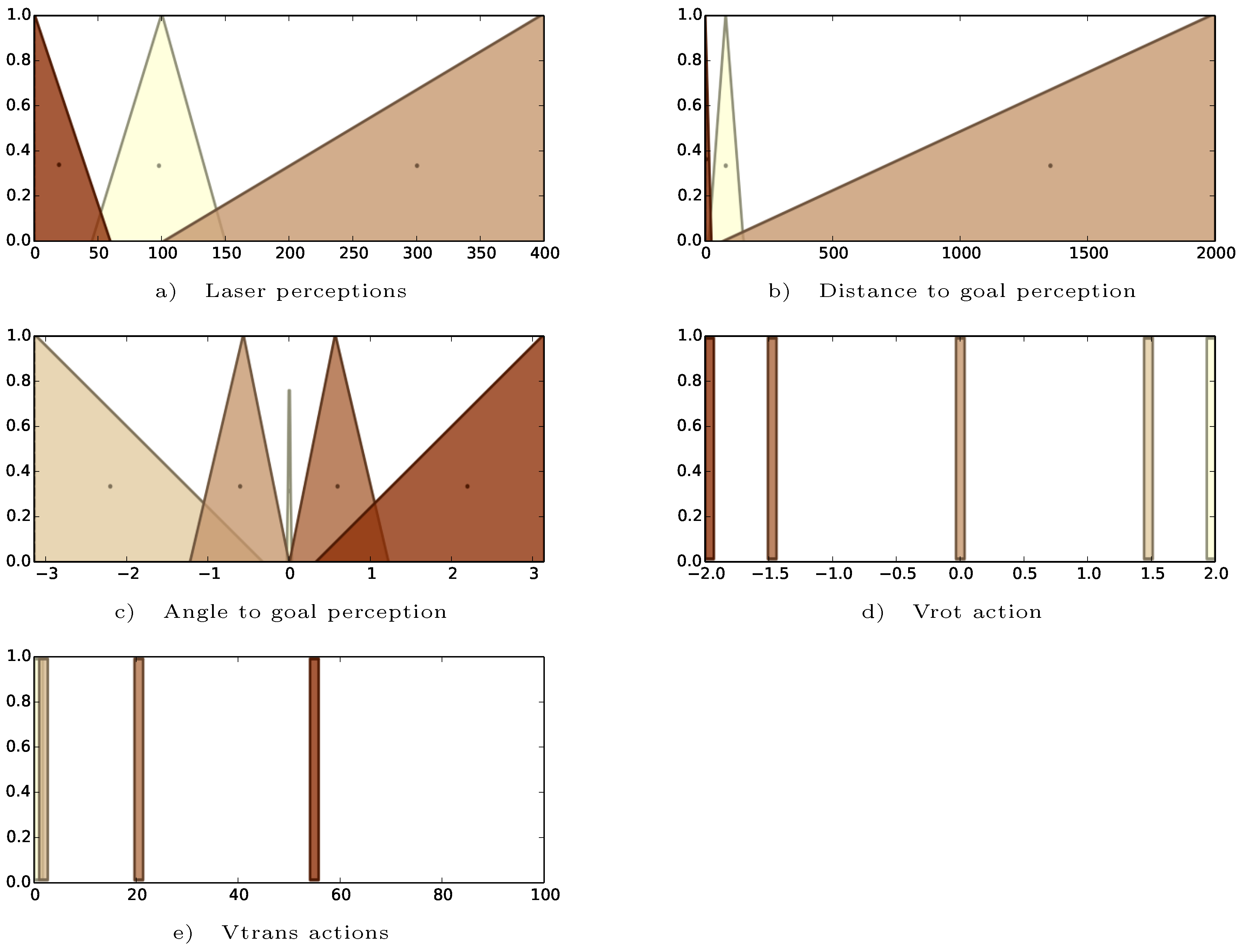
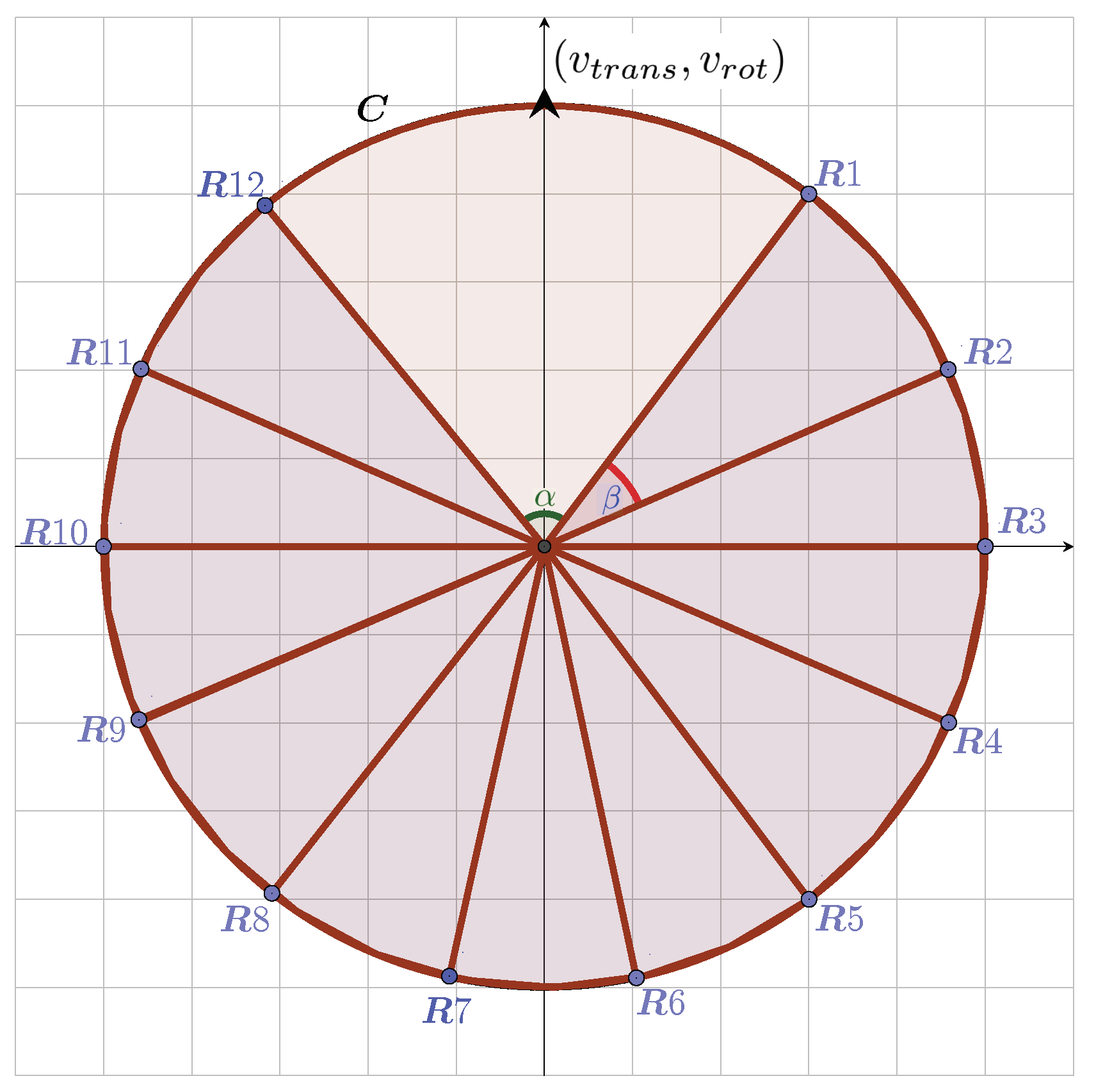
2.2. Low-Level Controller Design
Swarm Formation
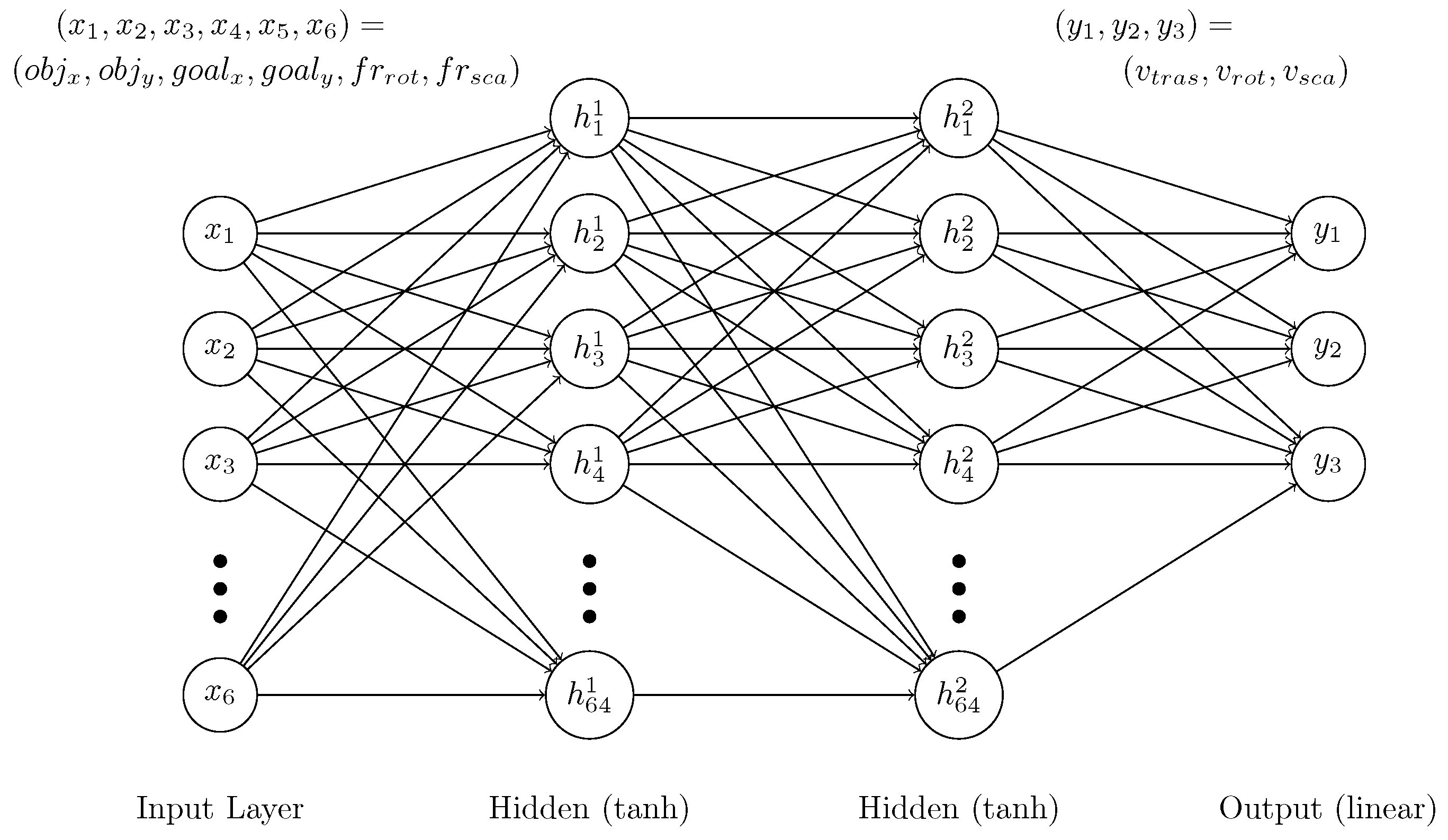
2.3. Reinforcement Learning Architecture
Markov Decision Process Design
3. Experiments
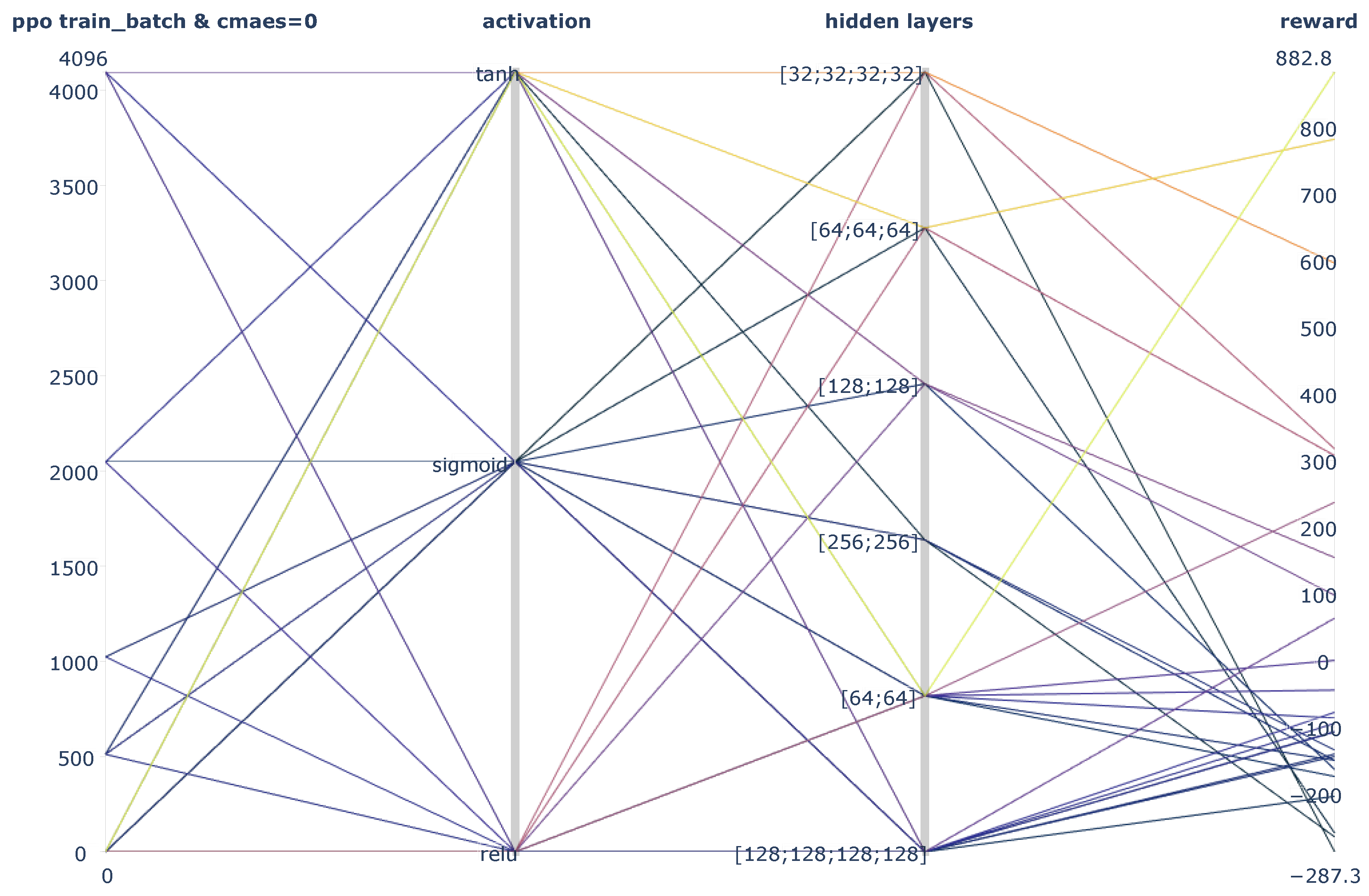
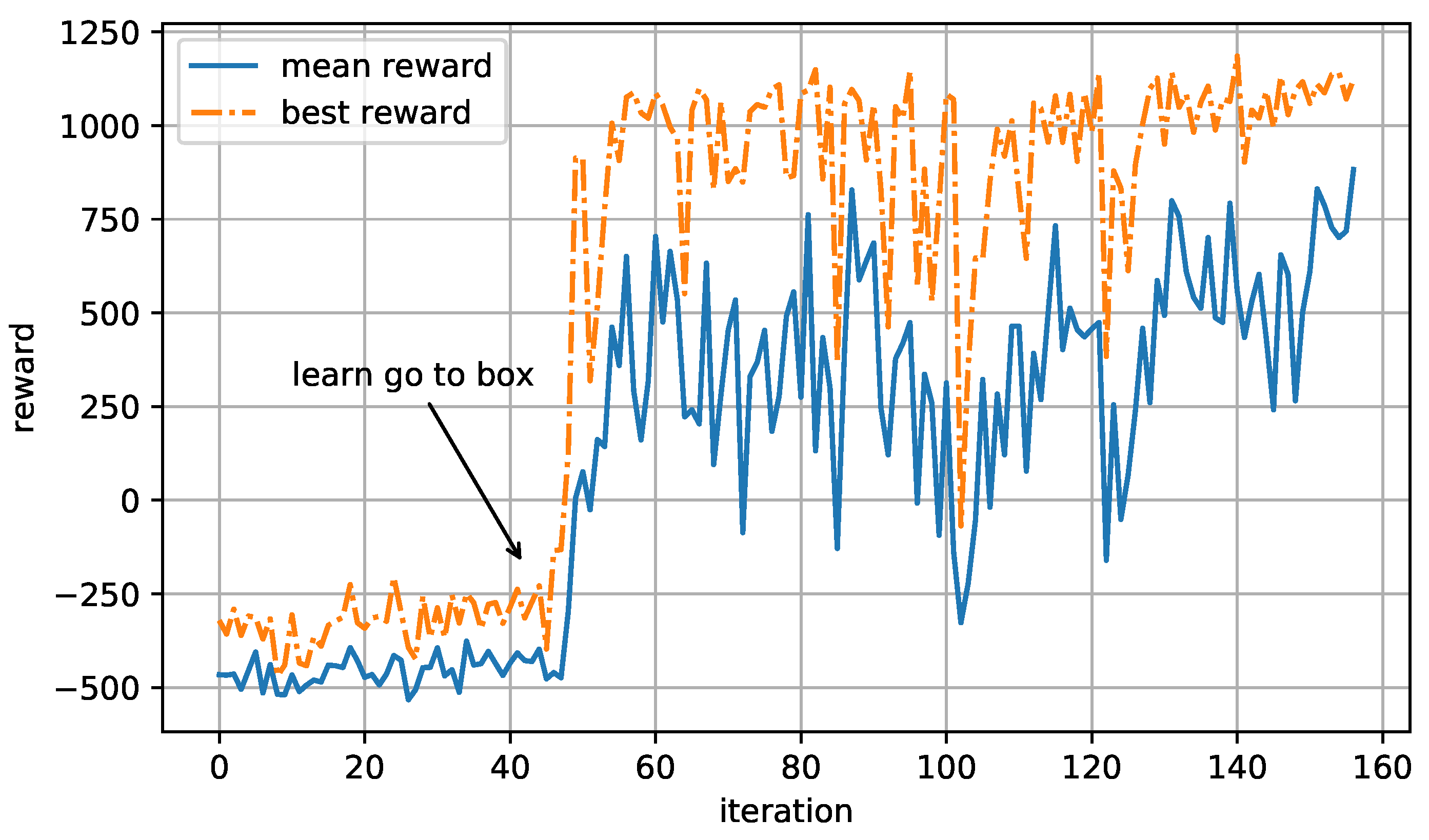
3.1. Training Phase
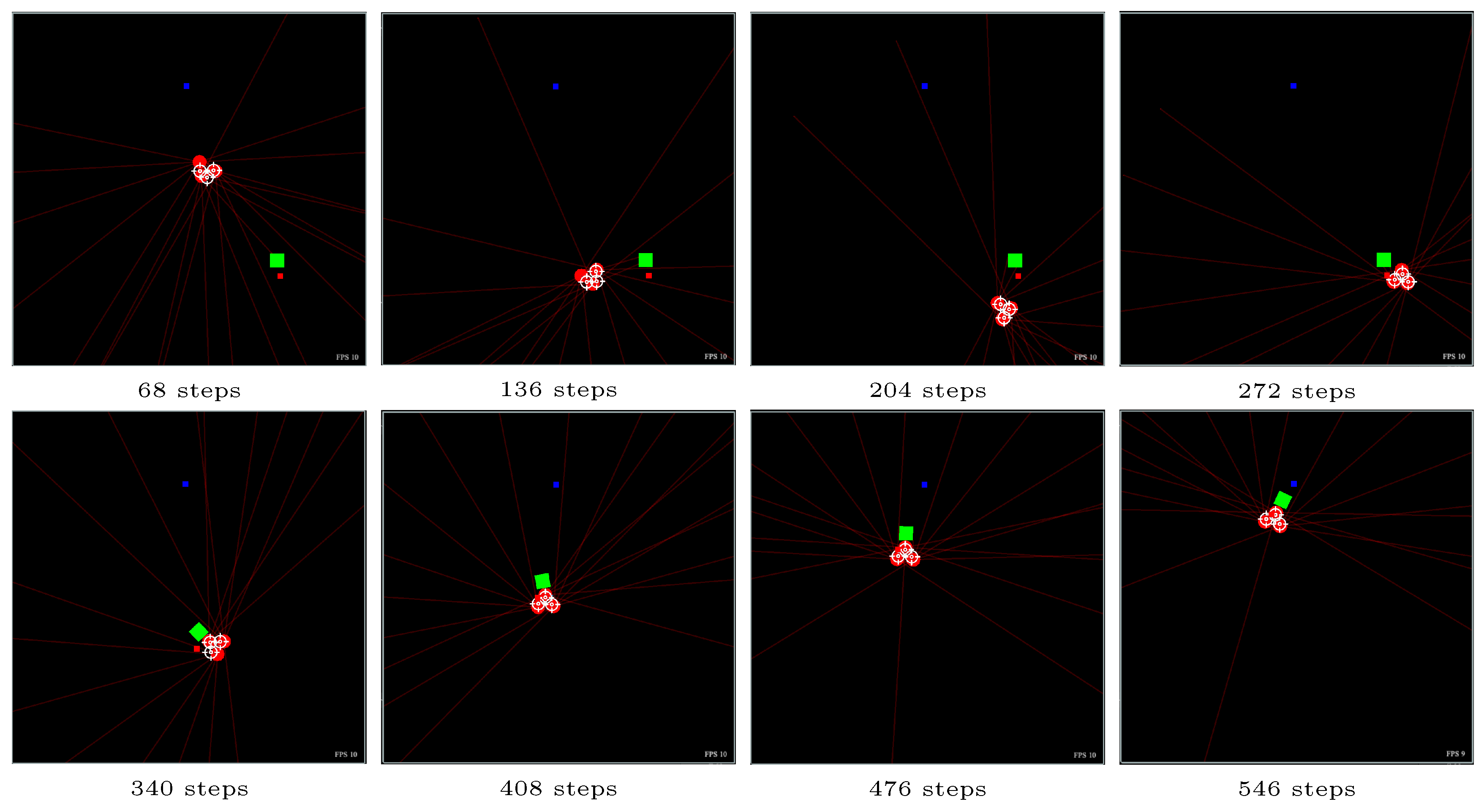
3.2. Evaluation Phase
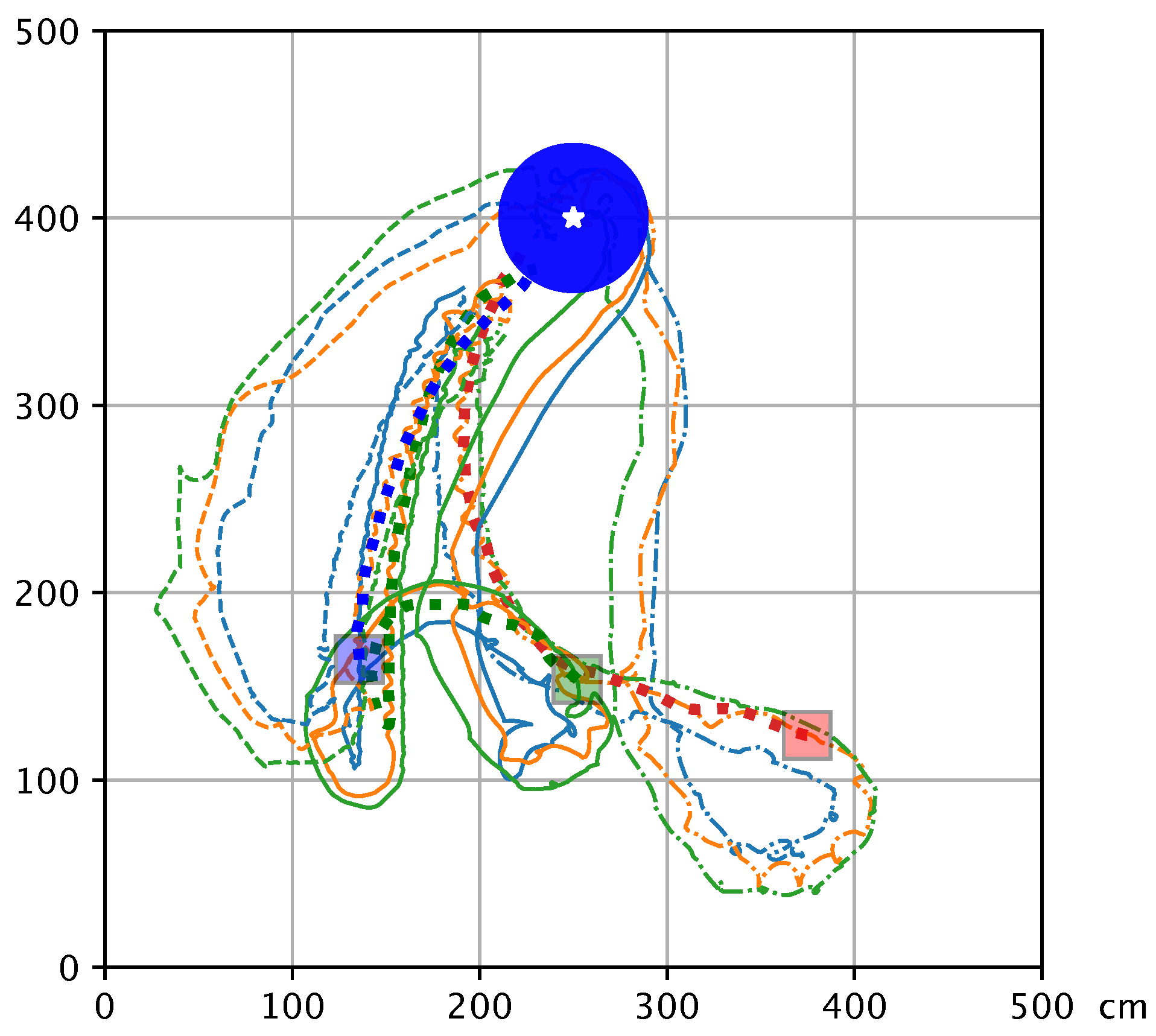
3.3. Scalability Tests
4. Discussion
5. Conclusions and Future Works
Author Contributions
Funding
Institutional Review Board Statement
Informed Consent Statement
Data Availability Statement
Conflicts of Interest
References
- Song, Y.; Fang, X.; Liu, B.; Li, C.; Li, Y.; Yang, S.X. A novel foraging algorithm for swarm robotics based on virtual pheromones and neural network. Appl. Soft Comput. 2020, 90, 106156. [Google Scholar] [CrossRef]
- Yogeswaran, M.; Ponnambalam, S.; Kanagaraj, G. Reinforcement learning in swarm-robotics for multi-agent foraging-task domain. In Proceedings of the 2013 IEEE Symposium on Swarm Intelligence (SIS), Singapore, 16–19 April 2013; pp. 15–21. [Google Scholar] [CrossRef]
- Barrios-Aranibar, D.; Goncalves, L.M.G. Learning to Collaborate from Delayed Rewards in Foraging Like Environments. Jornadas Peruanas De Computación JPC 2007. [Google Scholar]
- Iima, H.; Kuroe, Y. Swarm reinforcement learning methods improving certainty of learning for a multi-robot formation problem. In Proceedings of the 2015 IEEE Congress on Evolutionary Computation (CEC), Sendai, Japan, 25–28 May 2015; pp. 3026–3033. [Google Scholar] [CrossRef]
- Bernstein, A.V.; Burnaev, E.V.; Kachan, O.N. Reinforcement Learning for Computer Vision and Robot Navigation. In Machine Learning and Data Mining in Pattern Recognition; Perner, P., Ed.; Springer: Cham, Switzerland, 2018; Volume 10935, pp. 258–272. [Google Scholar] [CrossRef]
- Fathinezhad, F.; Derhami, V.; Rezaeian, M. Supervised fuzzy reinforcement learning for robot navigation. Appl. Soft Comput. 2016, 40, 33–41. [Google Scholar] [CrossRef]
- Efremov, M.A.; Kholod, I.I. Swarm Robotics Foraging Approaches. In Proceedings of the 2020 IEEE Conference of Russian Young Researchers in Electrical and Electronic Engineering (EIConRus), St. Petersburg and Moscow, Russia, 27–30 January 2020; pp. 299–304. [Google Scholar] [CrossRef]
- Hein, D.; Hentschel, A.; Runkler, T.; Udluft, S. Particle swarm optimization for generating interpretable fuzzy reinforcement learning policies. Eng. Appl. Artif. Intell. 2017, 65, 87–98. [Google Scholar] [CrossRef]
- Thrun, S.; Burgard, W.; Fox, D. Probabilistic Robotics; illustrated auflage ed.; The MIT Press: Cambridge, MA, USA, 2005. [Google Scholar]
- Gebhardt, G.H.; Daun, K.; Schnaubelt, M.; Neumann, G. Learning Robust Policies for Object Manipulation with Robot Swarms. In Proceedings of the 2018 IEEE International Conference on Robotics and Automation (ICRA), Brisbane, Australia, 21–25 May 2018; pp. 7688–7695. [Google Scholar] [CrossRef]
- Hüttenrauch, M.; Šošić, A.; Neumann, G. Guided Deep Reinforcement Learning for Swarm Systems. arXiv 2017, arXiv:1709.06011. [Google Scholar]
- Hüttenrauch, M.; Šošić, A.; Neumann, G. Deep Reinforcement Learning for Swarm Systems. arXiv 2019, arXiv:1807.06613. [Google Scholar]
- Tai, L.; Zhang, J.; Liu, M.; Boedecker, J.; Burgard, W. A Survey of Deep Network Solutions for Learning Control in Robotics: From Reinforcement to Imitation. arXiv 2016, arXiv:1612.07139. [Google Scholar]
- Schulman, J.; Wolski, F.; Dhariwal, P.; Radford, A.; Klimov, O. Proximal Policy Optimization Algorithms. arXiv 2017, arXiv:1707.06347. [Google Scholar]
- Hansen, N.; Ostermeier, A. Completely Derandomized Self-Adaptation in Evolution Strategies. Evolut. Comput. 2001, 9, 159–195. [Google Scholar] [CrossRef] [PubMed]
- Suttorp, T.; Hansen, N.; Igel, C. Efficient covariance matrix update for variable metric evolution strategies. Mach. Learn. 2009, 75, 167–197. [Google Scholar] [CrossRef]
- Salimans, T.; Ho, J.; Chen, X.; Sidor, S.; Sutskever, I. Evolution Strategies as a Scalable Alternative to Reinforcement Learning. arXiv 2017, arXiv:1703.03864. [Google Scholar]


| Behavior | N. | Antecedent | Consequent |
|---|---|---|---|
| Avoidance | A1 A2 A3 A4 A5 A6 | left is emer and right is emer and front is emer left is emer and right is emer and front is far left is emer and right is far right is emer and left is far left is near and right is far right is near and left is far | vrot is right vrot is none vrot is hright vrot is hleft vrot is right vrot is left |
| Rendezvous | F1 F2 F3 F4 F5 F6 F7 F8 F9 F10 | ang is near ang is medl ang is medr ang is farl ang is farr dist is far dist is med dist is near front is emer front is near | vrot is none vrot is right vrot is left vrot is hright vrot is hleft vtrans is high vtrans is medium vtrans is stop vtrans is medium vtrans is medium |
| Combination | C1..C6 C7..C17 | C: (dist is far or dist is med) and + A C7..17: F | Same as base behavior |
| Box Mass (g) | Correct Executions | Fail Distance Mean (cm) | Fail Distance Std (cm) |
|---|---|---|---|
| 500 | 81% | 236.92 | 90.78 |
| 1000 | 80% | 182.13 | 80.15 |
| 1500 | 83% | 171.59 | 90.75 |
| 2000 | 85% | 193.76 | 82.59 |
| Box Size (cm) | Correct Executions | Fail Distance Mean (cm) | Fail Distance Std (cm) |
|---|---|---|---|
| 10 | 70% | 264.94 | 147.51 |
| 20 | 80% | 182.13 | 80.15 |
| 30 | 68% | 182.12 | 85.18 |
| 40 | 29% | 167.12 | 65.69 |
| Num. Robots | Correct Executions | Fail Distance Mean (cm) | Fail Distance Std (cm) | CV |
|---|---|---|---|---|
| 2 | 65% | 173.68 | 75.54 | 43.49 |
| 3 | 80% | 182.13 | 80.15 | 44.00 |
| 4 | 83% | 192.22 | 113.61 | 59.10 |
| 5 | 67% | 221.05 | 114.64 | 51.86 |
| 6 | 64% | 216.78 | 125.35 | 57.82 |
| 7 | 59% | 223.71 | 130.62 | 58.38 |
| 8 | 40% | 236.16 | 123.38 | 52.24 |
| 9 | 30% | 258.02 | 137.79 | 53.40 |
| 10 | 37% | 241.39 | 134.42 | 55.68 |
Publisher’s Note: MDPI stays neutral with regard to jurisdictional claims in published maps and institutional affiliations. |
© 2021 by the authors. Licensee MDPI, Basel, Switzerland. This article is an open access article distributed under the terms and conditions of the Creative Commons Attribution (CC BY) license (http://creativecommons.org/licenses/by/4.0/).
Share and Cite
Aznar, F.; Pujol, M.; Rizo, R. Learning a Swarm Foraging Behavior with Microscopic Fuzzy Controllers Using Deep Reinforcement Learning. Appl. Sci. 2021, 11, 2856. https://doi.org/10.3390/app11062856
Aznar F, Pujol M, Rizo R. Learning a Swarm Foraging Behavior with Microscopic Fuzzy Controllers Using Deep Reinforcement Learning. Applied Sciences. 2021; 11(6):2856. https://doi.org/10.3390/app11062856
Chicago/Turabian StyleAznar, Fidel, Mar Pujol, and Ramón Rizo. 2021. "Learning a Swarm Foraging Behavior with Microscopic Fuzzy Controllers Using Deep Reinforcement Learning" Applied Sciences 11, no. 6: 2856. https://doi.org/10.3390/app11062856
APA StyleAznar, F., Pujol, M., & Rizo, R. (2021). Learning a Swarm Foraging Behavior with Microscopic Fuzzy Controllers Using Deep Reinforcement Learning. Applied Sciences, 11(6), 2856. https://doi.org/10.3390/app11062856