An Innovative Approach to Accuracy of Co-Seismic Surface Displacement Detection Using Satellite GNSS Technology

Abstract

This paper discusses a new method for determining co-seismic displacement using the Global Navigation Satellite System (GNSS) for the precise detection of positional changes at permanent stations after an earthquake. Positioning by the Precise Point Positioning (PPP) method is undertaken using data from the GNSS satellites and one designated station. A time series is processed by an anharmonic analysis before and after an earthquake and these one-day solutions increase the accuracy of measurements. The co-seismic static displacement can be precisely detected from the analysed time series before and after the earthquake, which can be used for the verification of seismic models. Reliability of the estimation of the size of the co-seismic offset is given by the mean square error (RMSE) of the shift. In this study, RMSE was determined by two approaches, initially from variances within PPP processing, and secondly when no positional change from the GNSS before or after the earthquake was assumed. The variance of the data in the time series gives a more realistic estimate of RMSE. This dual approach can affect seismological interpretation due to the need for the interpreting geophysicists to determine which case of co-seismic displacement is more probable for any given locality. The second approach has been shown to provide a more realistic co-seismic displacement accuracy in this study.

1. Introduction

Earthquakes represent a sudden rupture along faults loaded by tectonic forces. In large shallow earthquakes, the ruptured part of a fault rarely reaches the Earth’s surface and is measurable. The rupture process is usually entirely confined underground. Even if this is the case, off-fault, co-seismic displacements occur on the surface of the Earth. The co-seismic displacement has its dynamic (oscillatory) part, due to seismic waves, and a static part. Post-earthquake stress reduction causes viscous relaxation, afterslip and/or poroelastic rebound [1] (i.e., post-seismic displacement on the fault plane).

Well before the seismic instrument era, large, visible on-fault co-seismic static displacements of the order of centimetres or meters were documented (the seismic instrument era started at the beginning of 20th century). The first measurement of displacement (co-seismic and post-seismic) was possible due to the use of repeated triangulation in the San Francisco Bay area after the Hayward earthquake in 1868 [2]. Other co-seismic and post-seismic displacements were obtained from the repeated triangulation of the Nobi earthquake on the Japanese islands in 1891 [3]. Since the middle of the 20th century many attempts have been made to measure off-fault static co-seismic displacements by seismic methods using double integration of acceleration records. However, even contemporary attempts of this kind [4] are difficult due to low-frequency natural and instrumental noise. The advent of space-geodesy techniques at the end of 20th century in the form of Global Navigation Satellite Systems (GNSS), has considerably improved the off-fault measurement of earthquake-related displacements (co-seismic dynamic and static displacement, and post-seismic displacement). A study of a 20-year database of co-seismic displacements in Greece has been discussed by Ganas et al. [5]. Further progress has been provided by the introduction of In-SAR methods [6] whose main advantage is a dense (periodically every 6–12 days) sampling of the motion on the Earth’s surface over a large area [7,8]. In-SAR methods can also detect pre-seismic ground deformation, as demonstrated by Nardo [9]. It is our view that In-SAR methods will be used more frequently in the future. Other possibilities also may become apparent, especially in the field of earthquake prediction, when monitoring electromagnetic extra-low-frequency perturbations [10].

At this time, there is a very cooperative atmosphere in the field of seismology and space geodesy, especially within investigations of larger earthquakes (magnitude >~5), and in particular studies of slip evolution and distribution on faults. It is expected that future progress in this field will mainly be focussed on the continuous monitoring of known faults or broader areas. This will lead to better understanding of co-seismic processes, and post-seismic relaxation, or even a possible pre-seismic “earthquake preparatory phase”. Seismic and geodetic measurements can contribute to a better understanding of the rheological properties of fault zones (and their laws of friction), which remain enigmatic, hampering earthquake predictions, which is discussed in more detail by Ganas et al. [11,12].

The aim of this study is to determine the co-seismic displacement from a time series of coordinates determined by the PPP GNSS method and a realistic estimate of the accuracy for this co-seismic displacement. This estimate of accuracy evaluates the statistical significance of the determined displacement.

In this paper, Section 2 is an introduction to the geodetic monitoring of co-seismic displacement; in Section 3, a short introduction to the PPP method is given; the anharmonic spectral analysis for the coordinate time series is described in Section 4; Section 5 contains the processing of GNSS data and an error analysis of detected co-seismic displacements; the results are presented in Section 6; and Section 7 contains our conclusions.

2. Geodetic Monitoring of Co-Seismic Displacement

This paper focuses on a method to detect co-seismic static displacement during an earthquake by using precise positioning based on GNSS. We aim to provide a detailed description of the method used. Sokos et al. [13] applied the results of this method without giving any details of the method and Sokos et al. [14] only applied the results of the method as data in supplements without giving any details.

The method is based on the application of data from permanent GNSS stations, which continuously observe GNSS satellites. Based upon the results of these observations, the coordinates of the monitored stations in the global coordinate system can be determined at given intervals, and a time series of coordinates can be prepared and analysed. As discussed by Bevis and Brown [15], the time series of coordinates usually contain secular trends, annual oscillations, and rapid jumps. In case of an earthquake, the co-seismic static displacement of stations is calculated from the difference of the station position before and after the seismic event. The co-seismic displacement can be determined when analysing the time series before and after the earthquake. If a short part of the time series (i.e., two months maximum) is used, the secular trends and annual oscillations can be eliminated.

GNSS technology offers a variety of options to detect offsets. One type of GNSS data processing is the “relative network solution” method, where station coordinates are determined relative to reference stations located outside of an earthquake area. The deformation signal (i.e., co-seismic displacement) can also be extracted by analysing data from the entire GNSS network simultaneously using free-net solutions. Gautham et al. [16] used relative network solutions from the GAMIT/GLOBK software package and a Kalman filter to determine coordinates and to detect the rate of change in the station position. Xu K.K. et al. [17] introduced a method to extract spatially and temporally coherent signals by analysing data from the entire GNSS network simultaneously using free-net solutions. In this method, the deformation signal is extracted by analysing the change of the GNSS geometry net-form, integrating the location, baseline length, and directional information from all GNSS stations over the entire network. This is then combined with area strain, and the deformation characteristic is then further interpreted. When high-rate (10 Hz) recording GNSS receivers and accelerometers are located close to the fault where an earthquake occurs, the co-seismic dynamic shifts can be analysed [4]. However, this supposes the availability of a very dense network of high-rate GNSS stations and accelerometers.

Our aim was to analyse the data from a single station or from a few (2–5) stations in a large area around an earthquake hypocentre. Our method design was based on an approach different from the above-mentioned methods and our focus was based on the determination of coordinates using the PPP (Precise Point Positioning) method. From a comparison of the two methods, PPP and a “relative network solution”, Kostelecky et al. [18] concluded that virtually identical results are achieved using both methods.

In order to achieve the required positional accuracy, data from a single day was used. This means that the coordinates of the permanent station were determined every day. Twardzik et al. [19] noted that by using a kinematic precise point positioning strategy to determine co-seismic deformation within 12 h after an earthquake, the co-seismic displacement data may also contain early post-seismic deformation. This must not be overlooked during the evaluation of results.

An anharmonic analysis (described in more detail in Section 3) was used to analyse the time series of coordinate components (North, East, Up). Another possible way to analyse a time series of coordinates from the processing of long-term GNSS observations is to form baselines between stations and then analyse the rates of length change as demonstrated by Chousianitis et al. [20], using a Kalman filter.

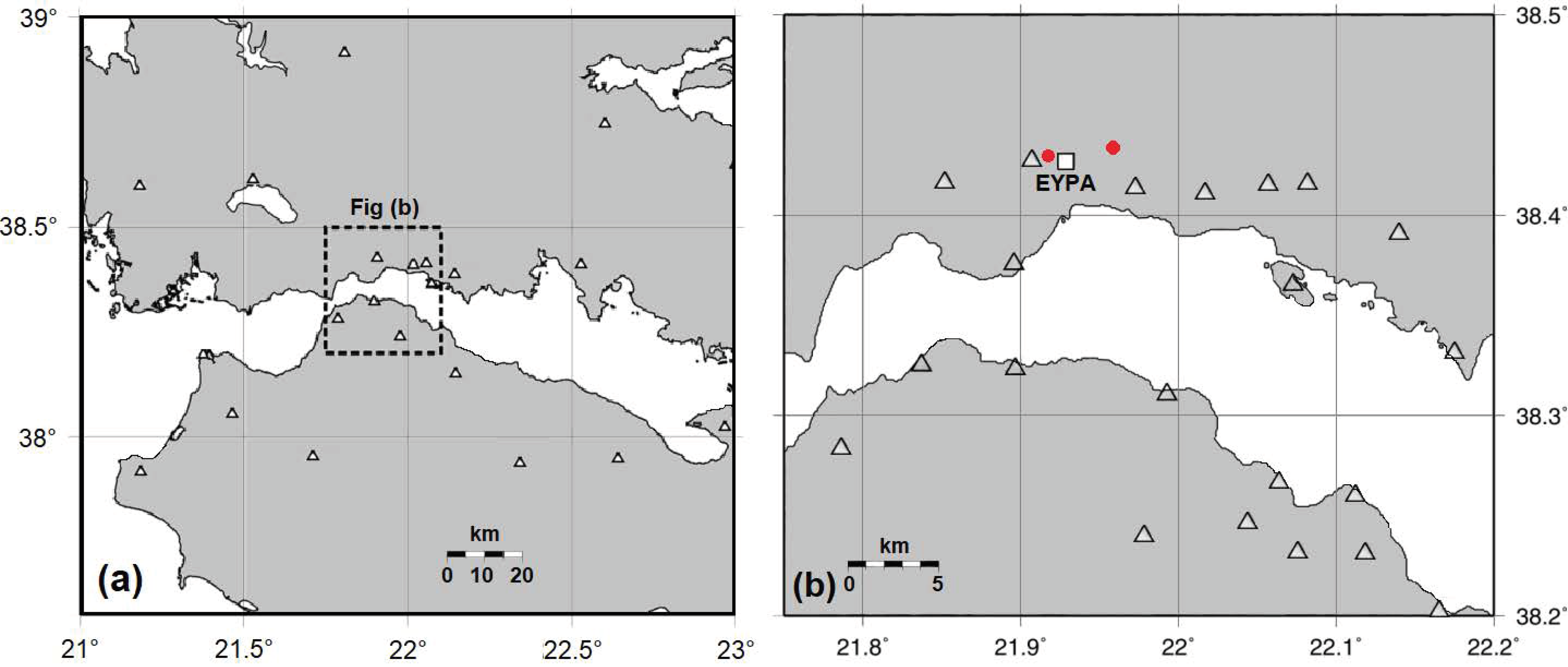
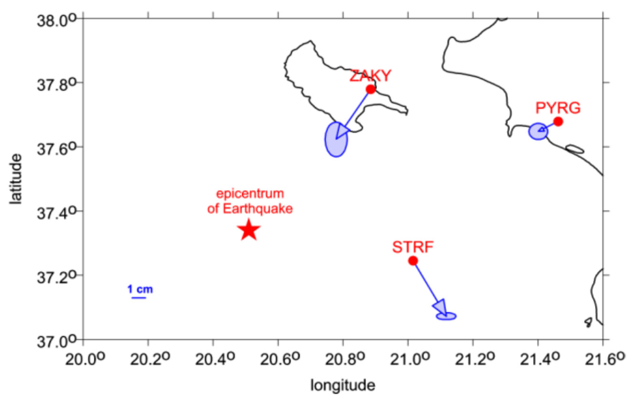
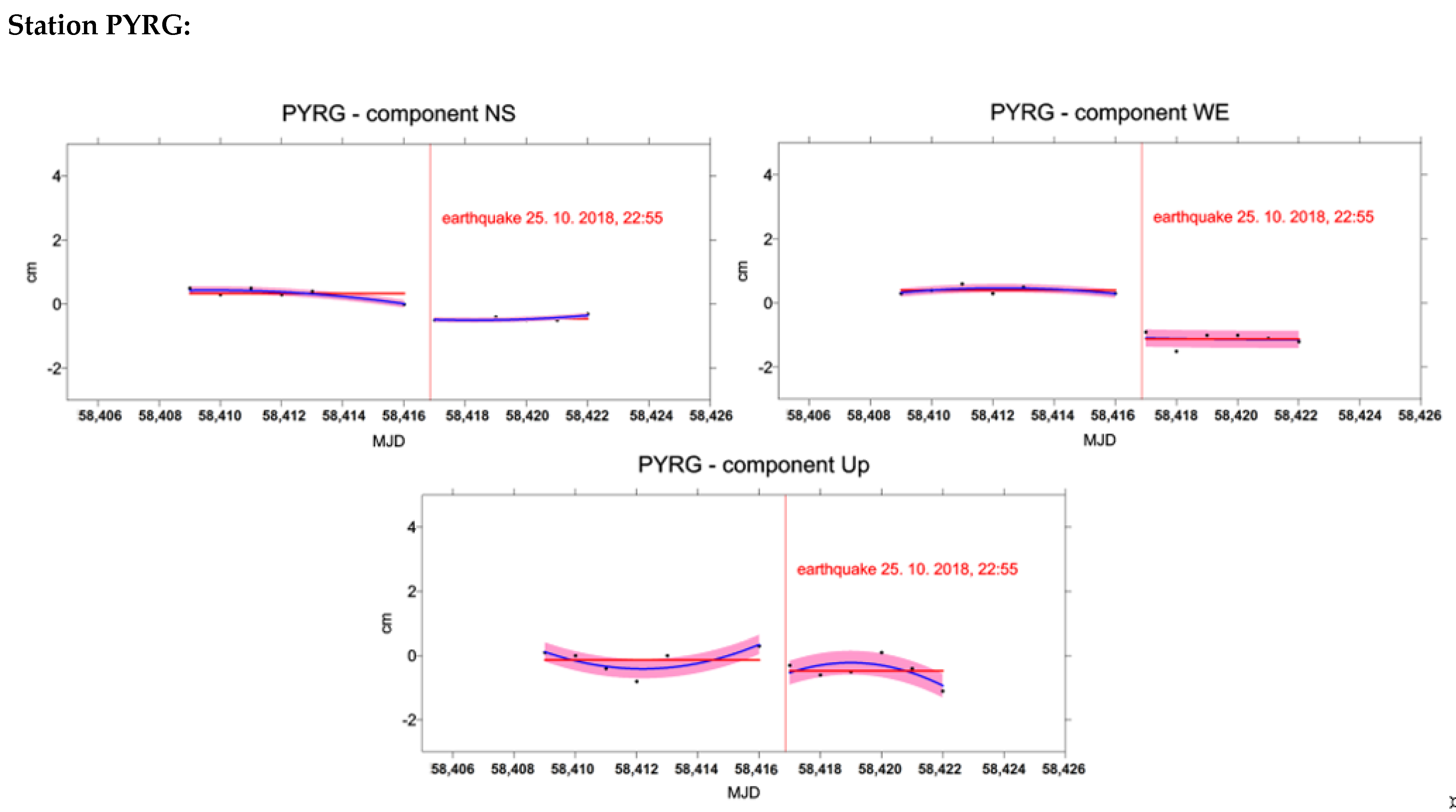
In this paper, we will focus on the displacement of permanent stations in Greece during the January 2010 earthquake in Efpalio [13] and the October 2018 earthquake located south of the island of Zakynthos [14]. In contrast to more significant earthquakes, (e.g., Tohoku-Oki with Mw 9.0, where the co-seismic shifts were on a metre level [16] and recorded more shifts in the afterslip phase [19]), the earthquakes in Efpalio and near Zakynthos were relatively small and without or with a very short afterslip phase (shorter than one day). Due to their post-seismic displacements being on a centimetre-level (i.e., close to the accuracy of GNSS method), we also focussed on determining the accuracy of the detected co-seismic displacements based on the results of an anharmonic analysis.

The aim of this study was to determine co-seismic displacement and its accuracy, using the mean square error of the difference between two calculations determined by the application of the PPP method. Each of the calculations are derived from the time series, before and after the earthquake. These are determined from an anharmonic spectral analysis of coordinates from the relevant section of the time series.

3. A Short Introduction to the PPP Method

The Precise Point Positioning (PPP) method [21] is based on the availability of accurate GNSS satellite coordinates and clocks. It uses models with centimetre precision to remove systematic effects on estimated parameters. For accurate GNSS satellite coordinates and clocks, the products from IGS (International GNSS Service—https://www.igs.org/data-products-overview/ [Accessed at 17 January 2021]) [22] were used. The most precise final orbit and clock products available two weeks after the last observation of the GPS week (a week from Sunday to Saturday) were used. Although the accuracy of the GNSS orbits and clocks are vital to achieving the highest level of PPP accuracy, the quality and type of processed GNSS observation is also critical. The highest positioning accuracy is achieved with geodetic quality, dual-frequency GNSS receivers operating in a low multipath environment where carrier phase cycle slips are infrequent.

3.1. Precise Point Positioning Correction Models

Developers of GNSS software are generally aware of the corrections they must apply to code (pseudorange) or carrier (phase) observations to eliminate effects such as special and general relativity, Sagnac delay, satellite clock offsets, and atmospheric delays. All of these effects are quite significant and can exceed several metres. They must be considered for pseudorange positioning at the metre precision level. Therefore, when attempting to combine satellite positions and clocks with a precision of a few centimetres with ionospheric-free carrier phase observations (with millimetre resolution), it is very important to account for some of these effects which may be neglected in code or precise differential Carrar processing.

The corrections that need to be made are ([21]):

• Satellite antenna: To account for the distance between the satellite centre of mass, to which the satellite coordinates are referred, and the phase centre of the antenna, from which observations are measured. The magnitude of potential error is at the level of metres.
• Phase Wind-Up: To account for a change in phase measurement due to the satellite rotating around its vertical axis during noon-turn and eclipse. The magnitude of potential error is at the level of decimetres.
• Solid Earth Tides: To account for the periodic displacement of the Earth’s crust due to the sun and moon. The magnitude of potential error is at the level of decimetres.
• Ocean Loading: To account for the deformation of the Earth’s crust caused by the increased load of water along coasts resulting from tidal action. The magnitude of potential error is at the level of centimetres.
• Relativity correction: To account for the effect of relativity on the GNSS onboard atomic clocks. The magnitude of potential error is at the level of metres.
• Pseudo-Range: This depends on pseudo-range observations with respect to the clock. The magnitude of potential error is about 2 ns of the user’s clock.
• Receiver antenna: To account for receiver antenna phase centre variations. The magnitude of potential error is at the level of centimetres.

In addition to applying correction models, atmospheric delays must be modelled, eliminated, or estimated. First-order ionospheric delay is eliminated using ionosphere free linear combinations of dual-frequency observations. The troposphere effect (tropospheric zenith delay) is modelled using default surface temperatures, and pressures adjusted to reflect antenna height and mapped along the signal path using the Niell Mapping Function [23].

4. Time Series Analysis Method

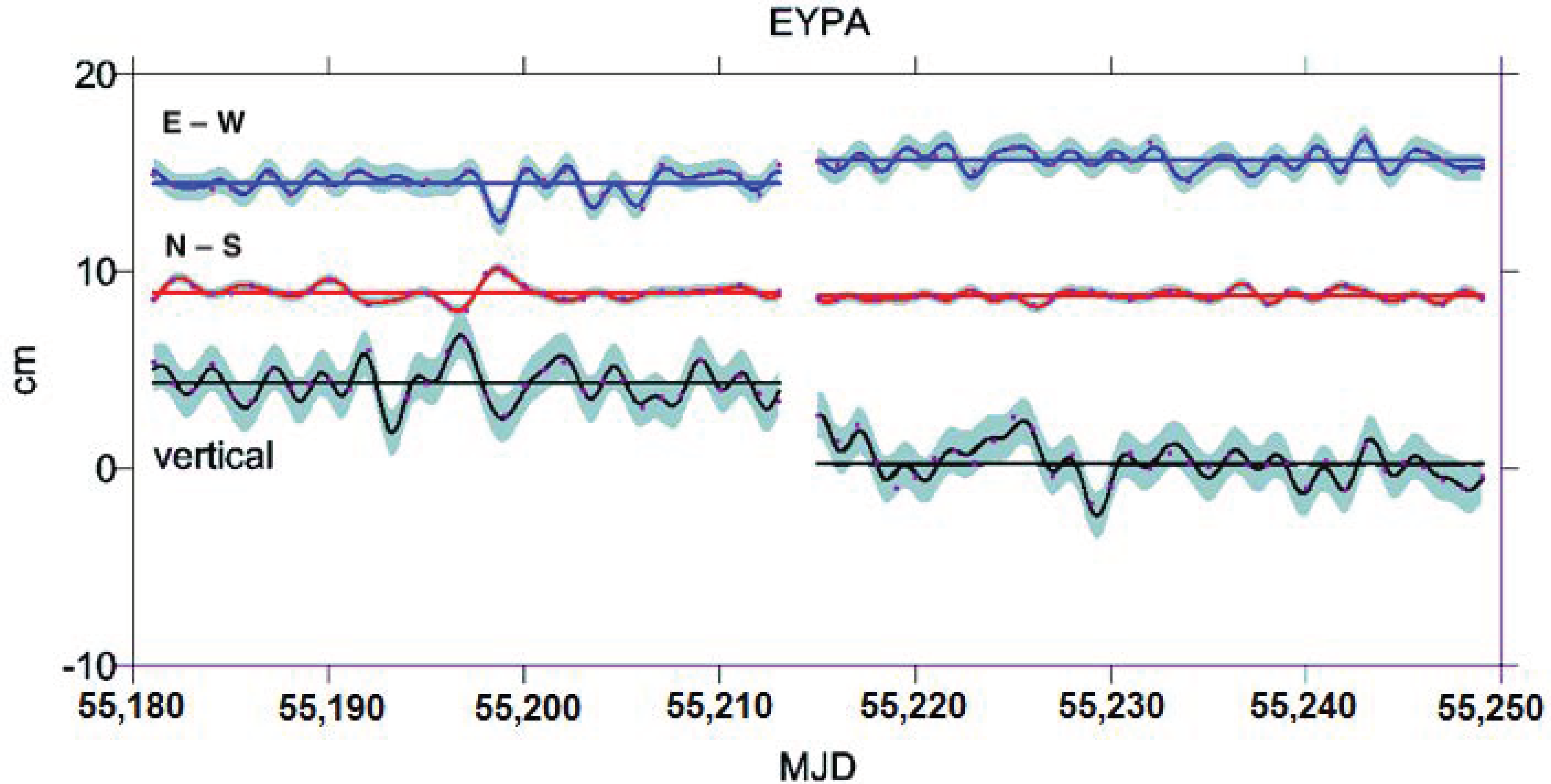
The main benefit of using the anharmonic spectral analysis method, described below, is that it suppresses the effect of the aliasing of possible periodic residues from imperfect models used for the elimination of systematic errors in the processing of GNSS data by PPP (see Section 3.1). The behaviour of the time series, which shows the features of repetition, can be observed in Figure 1. This shows the components, from W to E and Up, where the daily values of the coordinates show a near-periodic behaviour (which is often regarded as noise).

4.1. Spectral Analysis

The sets of homogenised values T and H(T) are considered the only realisation of the random process, which is considered to be ergodic. Preliminary analyses of the observation series indicated that the process is not normal and that it contains a determining component. Drawing on the physical characteristics of the process, it can be expressed in terms of a function of time t:

$$H_i\left(T\right)={{\displaystyle \sum }}_{k=0}^K{A}_k{t}_i^k+{{\displaystyle \sum }}_{j=1}^J{R}_{j}cos\left[2\pi f_j{t}_i-{ }^0{\varphi }_j\right]+s_i\left(t\right)$$

(1)

where $s_i\left(t\right)$ has a normal distribution with dispersion σ² and a mean value of ${\mu }_s\left(t\right)=0$, $A_k$ are polynomial coefficients, $f_j=1/P_j$ is the frequency, $P_j$ the period (in days), $R_j$ the amplitude, and ${ }^0{\varphi }_j$ the phase. Our method sought to seek the optimal estimate of these parameters, preserving the ergodic conditions and the realisation of properties (1) of the process. We also introduced the notations:

$${\sum }_{k=0}^K{A}_k{t}_i^k=Q_k, R_{j}cos\left[2\pi f_j{t}_i-{ }^0{\varphi }_j\right]=Q_j$$

(2)

In seeking the hidden periods, periodograms of the type:

$$I\left(f\right)={\left(2\pi T\right)}^{-1}{\left|{\int }_0^{T}x\left(t\right) exp\left(-itf\right)dt\right|}^2,$$

(3)

are usually used as a criterion in which f is the frequency, and x the continuous realisation of the random process in the interval T, $i=\sqrt{-1}$. However, we used a slightly different procedure for seeking hidden periods, which was Vaníček’s anharmonic analysis [24], as modified by Vondrák [25] and Kostelecký and Karský [26].

According to Tétreault et al. [27], the optimum spectrum (normalised to the interval <0, 1>), using (2) reads:

$$\sigma \left(x_i\right)=1-\left[\varrho \left(x_i-Q_k, Q_j\right)/\varrho \left(x_i, Q_k\right)\right]$$

(4)

where:

$$\varrho \left(F,G\right)={{\displaystyle \sum }}_{t\in T}{\left[F\left(t\right)-G\left(t\right)\right]}^2$$

(5)

defines the metric of the two functions F and G defined by T. The normalised spectrum enables an unambiguous determination of the significance of individual periods according to the selected fixed criterion.

The coefficients $A_k$ of polynomials $Q_k$ are determined under the assumption of independence, so that:

$$\varrho \left(x_i, Q_k\right)=min.$$

(6)

and, similarly, coefficients $R_j$ and ${ }^0{\varphi }_j$ from $Q_j$ are determined for every frequency $f\in \mathsf{\Omega }$, where $\mathsf{\Omega }$ is a set of reasonably optional frequencies, so that:

$$\varrho \left(x_i-Q_k, Q_j\right)=min$$

(7)

Coefficients $R_j$, j = 1, …, J, are therefore functions of frequency f_j, and as regards to $\sigma \left(x_i\right)$, it is easy to prove that for the given realisation of the process:

$$\sigma \left(x_i\right):\mathsf{\Omega } \to \langle 0 , 1\rangle$$

(8)

The separate maxima of function $\sigma \left(x_i, t\right)$, the spectrum peaks, determines the frequencies which make the principal contribution to the overall variation of the function $x_i\left(t\right)-Q_k\left(t\right).$ Conditions (6) and (7) lead to the traditional method of least squares adjustment. The value of K is determined in (1) and (2) from the already known character of the function or the empirical computation.

The described method entails finding the most significant wave first and filtering it by subtracting it from the original data. The difference is used as new input data and the next most significant wave is searched for. This is repeated until the maximum value of all found waves of the normalised spectrum is greater than the specified fixed criterium (e.g., 0.3).

4.2. Comments Concerning Real Computation

The algorithm described by the above relations was programmed using the FORTRAN computer language. Frequency $f_j=1/P_j$, ($P_j$ = the period in days) is chosen with a given step of $\Delta lnf$ (in the initial search for the period at a standard 0.01, and in the next search round specifying at 0.001), which implies the period discrimination:

$$\mathsf{\Delta }{P}_j\cong P_j \mathsf{\Delta }lnf$$

(9)

and a constant relative error. This method was adopted to be able to operate at reasonable computer speeds with the broadest range of periods possible being viewed. Equation (9) has to be used in evaluating the periods found; however, they accurately enter Equation (2) as the periods “found earlier”. The set Ω of optional frequencies can be automatically found within the range:

$$ln{f}_{min}\cong ln\left(\frac{1}{T}\right), ln{f}_{max}\cong ln\left[\left(n-1\right)/2T\right] ,$$

(10)

where T is the whole interval in days and n the number of observations. The approximate sign ≅ indicates rounding off with respect to (9) and the given $\Delta lnf$. In specifying the periods (with smaller than $\Delta lnf$) the range of periods $P_{min} , P_{max}$ can be chosen directly in the vicinity of their preliminary determined values. The degree of the polynomial, $K\ge 0$, is also always given.

5. Processing of GNSS Data

5.1. Data Source and Processing

Our area of interest is located within the seismically active regions of Greece, where medium-strong earthquakes are relatively frequent. In Greece, in addition to the seismic network, a dense network of permanent GNSS stations has been built to detect earthquakes (and subsequent tectonic movements). Raw data from GNSS stations are usually not freely available. However, access to the raw GNSS data was gained through cooperation with the Research Institute of Geodesy, Topography and Cartography at Zdiby, the Department of Geophysics at Charles University in Prague, and the University of Patras in Greece.

Data from permanent GNSS stations, located near the epicentre of the earthquake, were available to analyse the surface displacement caused by an earthquake. Data produced by the GNSS receiver in Compact RINEX format were available for the analysis. In all cases, full-day files with a 30 s data sampling rate were collected. Satellites of the U.S. GPS-NAVSTAR system and the Russian GLONASS system were used during the observations. Datasets were available several days (between 5 and 30) before and after the earthquake.

Data processing, to acquire observation station coordinates, was performed using the PPP method, detailed in Section 3. Freely accessible software [27] from the Canadian geological service NRCan (Geodetic Survey Division, Natural Resources Canada) was used. GNSS satellite precise ephemeris and onboard clock corrections, published with a 14-day delay by IGS (International GNSS Service), were used to determine station coordinates. Satellite ephemeris accuracy is currently at 3 cm in position and 1 ns in satellite clock correction. The necessary calibration and atmospheric corrections for individual observations were determined from the models. The method continued to operate through the iteration process. For each day-long data set, results characterised by internal accuracy (with 95% probability) in the NS (north-south direction): 2–3 mm, in the WE (west-east direction): 4–6 mm and in the Up (vertical direction): 8–12 mm, were obtained.

One result was available for each day’s file. Therefore, it was possible to analyse the time series in the interval before and after the earthquake. Anharmonic analysis, detailed in Section 3, was used. Based on the time series analysis before and after the earthquake, the differences that express the co-seismic displacement of the stations caused by the earthquake were determined. A prerequisite is that during the earthquake, the GNSS antenna on the station was not moved with respect to the background, and results of the analysis represent a displacement of the surface.

5.2. Analysis of the Shift Error

As mentioned above, the co-seismic displacement is calculated as the difference in the averaged position of the station before and after the earthquake. An important variable to compare with the result determined from the seismic model is its mean square error (RMSE). The RMSE defines whether the size of the co-seismic displacement is statistically significant. In our case, it was calculated as the RMSE of the difference between the two values.

However, we can use two approaches to calculate the mean error value:

The first approach:

Assume that the mean quadratic errors of the positions determined from the application of the PPP method are real, and that they characterise the estimated actual variance. We can then assume that something happens with the GNSS before and after the earthquake and that the subsequent analysis of the time series gives us a realistic approximation of the station’s behaviour after the earthquake. The mean square error of the approximation curve is considered a real estimate of the RMSE 1st approach.

The second approach:

We assumed that the mean quadratic errors (RMSE) determined from the application of the PPP method are considered to be overestimated, and that they can only be considered internal mean errors. The assumption is that nothing happens with the GNSS station before or after the earthquake (it is not affected by post-seismic displacements). The dispersion of the approximation data from the time series analysis is given by the real errors of the individual daily results. This differs from the determination of RMSE from the PPP method. We also need to make the assumption that the time series is a random statistical process. When calculating the RMSE of the difference before and after the earthquake, in the RMSE 2nd approach, it is taken into account that the resulting mean square error of the difference is calculated based on the variance of individual observations.

In

Table 1. Co-seismic displacement of the EYPA station position, as determined by GNSS observations (using the anharmonic spectral analysis) with RMSE from both approaches and the comparison with the static displacement calculated from the COULOMB 3.1 seismic model [13], with the difference between the averages of the daily GNSS results.

Determined Shift	Co-Seismic Displacement from Anharmonic Analysis	RMSE of GNSS (1st Approach)	RMSE of GNSS (2nd Approach)	Static Displacement from Seismic Model	Difference between the Averages of Daily Results
N-S	−0.13 cm	0.02 cm	0.48 cm	−0.31 cm	−0.22 cm
E-W	1.22 cm	0.07 cm	0.76 cm	0.78 cm	1.15 cm
Up	−4.10 cm	0.10 cm	1.38 cm	−3.12 cm	−4.04 cm

and

Table 2. Results of time series analysis before and after the earthquake in Zakynthos area with RMSE from the 1st and 2nd approaches.

Station	NS [cm]			EW [cm]			Up [cm]
	Offset	RMSE 1st Approach	RMSE 2nd Approach	Offset	RMSE 1st Approach	RMSE 2nd Approach	Offset	RMSE 1st Approach	RMSE 2nd Approach
STRF	−4.33	0.03	0.09	2.55	0.08	0.25	0.66	0.16	0.38
ZAKY	−3.89	0.20	0.45	−2.65	0.10	0.28	−0.70	0.30	0.75
PYRG	−0.78	0.08	0.21	−1.52	0.08	0.24	−0.35	0.22	0.56

, the RMSE calculated using the 2nd approach was greater than the RMSE calculated by the 1st approach. It is usually 2–3 times larger, but in some cases (NS component in Table 1), it is even 24 times greater. We found that the RMSE calculated according to the 1st approach is not applicable for evaluating the statistical significance of the calculated co-seismic displacement.

6. Application of the Method on Two Earthquakes in Greece

Our study focused on the detection of the displacement of permanent stations during the January 2010 earthquake in Efpalio [13] and the October 2018 earthquake located south of the island of Zakynthos [14]. The results of the methods were applied without any details in [13,14] with the aim of modelling the tectonics in earthquake areas.

6.1. Efpalio Earthquake

6.1.1. EYPA Station in the Efpalio Area

The Corinth Gulf in Greece is frequently disrupted by earthquakes. In order to detect them, a network of permanent and temporary seismic stations has been deployed across the area. The region also hosts one permanent GNSS station. The geographical distribution of the permanent observing stations is shown in Figure 2.

On 18 January 2010, an earthquake occurred in the Efpalio area, with a magnitude of Mw 5.3. Its epicentre was close to the GNSS permanent station EYPA. A second moderate size earthquake (Mw 5.2) occurred on 22 January 2010; its epicentre was about 5 km from the EYPA station. These two most significant events were accompanied by a sequence of aftershocks that lasted for almost six months. Both M5+ shocks exhibited normal faulting along ~E-W trending planes.

6.1.2. Co-Seismic Displacement Computations and Their Accuracy

The different horizontal (E-W, N-S and Up coordinate differences using the PPP method are plotted in Figure 1. The time on the x-axis is expressed in Modified Julian Date (MJD). The coordinate difference time series are approximated using the method found in Section 4. The result shows systematic offsets in both the E-W and the Up directions (up to 40 mm). The RMSE of the daily solution is characterised by 3 mm, 6 mm, and 11 mm in N-S, E-W, and Up directions, respectively.

To estimate systematic offsets between the mean coordinates before and after the earthquake (i.e., co-seismic static displacement), we used an anharmonic analysis, but with estimating constant members. Additionally, the critical day of 18 January 2010 (MJD 55214) was excluded from the analysis. The result of this analysis is shown in Figure 3, and the estimated differences of the individual components can be seen in Table 1 with RMSE computed using both approaches.

The result of the most commonly used method for determining the magnitude of the displacement (i.e., the difference between the averages of the daily GNSS results before and after the seismic event) is also given in Table 1. It is evident that they differ (by +0.09 cm, +0.07 cm, −0.06 cm) from the result of the anharmonic spectral analysis. In the N-S direction, this is more than RMSE from the 1st approach. Therefore, in some cases, there is a difference between determining co-seismic displacement from the differences in arithmetic averages and the differences in anharmonic spectral analysis.

RMSE from the 1st approach are less than or equal to 1 mm (0.2, 0.7, 1.0 mm for the components N, E, Up). This is an order of magnitude less than the usual positioning accuracy of PPP. RMSE from the 2nd approach (4.8, 7.6, 13.8 mm for the components N, E, Up) are several times larger (24×, 11×, 13× for the components N, E, Up). Therefore, they better correspond to the assumed accuracy of determining the difference from PPP positions.

6.1.3. Comparison with Seismological Results

The EYPA position changes derived from the GNSS observations have been seismically interpreted (see [13]). The seismic model, consisting of the centroid moment tensor solution and a simple planar fault with a constant slip, has been processed with the COULOMB v. 3.1 software (by colleagues from Charles University in Prague [13]). The results from the GNSS measurements (co-seismic displacement was calculated after both earthquakes) and from the static model (only for 18 January event) are summarised in Table 1. The difference of both displacements (+0.18 cm, +0.44 cm, −0.98 cm) is below the RMSE of GNSS (2nd approach). This again shows that the 2nd approach for computing the RMSE gives a more realistic estimate than the RMSE from the 1st approach. Sokos et al. [13] states that there is a relatively good agreement between the results of anharmonic analysis and the accuracy given by the 2nd approach. The difference of both displacements may also be caused by post-seismic displacements that occurred shortly after the earthquake, which the static seismic model does not consider.

6.2. Stations in Zakynthos Area

On 25 October 2018, at 22:54 UTC, a Mw 6.8 earthquake occurred in the sea, south-west of Zakynthos Island (Lat 37.34°, Lon 20.51°; see Figure 4) [14]. It caused some damage to the island, but there were no casualties. There was large-scale monitoring of the event, and Ganas et al. [12] indicate that this event ruptured the Hellenic megathrust.

Co-Seismic Displacements at the Three Closest Stations

Data from three permanent GNSS stations, not far from the epicentre of the earthquake, were available to analyse the surface shifts caused by the earthquake. These are the PYRG (Pyrgos), STRF (Strofades), and ZAKY (Zakynthos) stations. Raw GNSS data sets were available 5 (or 6) days before and five days after the earthquake. Data processing, leading to the acquisition of observation station coordinates, was performed using the PPP method, described in Section 3.

Time series analyses for all three stations was performed using the anharmonic spectral analysis method (Section 4). From the analysis of the time series during the earthquake (see series of Figure 5), it can be seen that in all cases, station offsets occurred during the earthquake. Therefore, the appropriate series before and after the earthquake were analysed for co-seismic displacement. In Figure 5, these lines are highlighted in red.

Figure 5 shows the time series of coordinates with a total length of 10 to 12 days. The anharmonic spectral analysis is shown to detect a maximum of one major period, which are represented by the blue curves. The co-seismic displacements are determined from the differences between the averaged values (red lines). The calculated variances are characterized by the pink belts.

Subsequently derived co-seismic displacements from the approximation curve differences “before and after” can be found in Table 2 with different computations of RMSE using both approaches (see Section 5.2).

The RMSEs from the 1st approach are less than 3 mm, and on average 1.4 mm. This is more than in the previous example and this is because the processed time series of coordinates are shorter (5 days vs. more than 30 days). RMSEs from the 2nd approach (from 0.9 to 7.5 mm, with an average of 3.6 mm) are 2 to 3 times greater than the RMSEs from the 1st approach. RMSE from the 2nd approach better corresponds to the usual accuracy of determining the difference from PPP positions.

Considering the 99.7% confidence level, the deviation limit is calculated as 2.95 times the RMSE. The components N and E at all of the stations are greater than the deviation limit and can be considered as determined. The opposite is the case for the Up components. Their limit deviations (1.12, 2.21, 1.65 cm for the STRF, ZAKY, and PYRG stations respectively) are larger than the absolute values of the Up components of the co-seismic displacement (0.66, 0.70, 0.35 cm for the STRF, ZAKY and PYRG stations respectively). Therefore, we do not consider them to be reliably determined.

The distribution of the stations with the resulting vectors are shown in Figure 4. Values of 2.95 sigma (2nd approach) are depicted at the end of the vector of horizontal shifts.

As we have already stated, the 2nd approach for RMSE shows that the vertical component of the co-seismic displacement cannot be detected accurately. Sokos et al. [14] compared the horizontal components of co-seismic displacement (computed from GNSS data) with seismic source model results for the Zakynthos earthquake. They state that the horizontal displacement of the ZAKY and PYRG stations agrees with the seismic source model. The horizontal displacement determined at the STRF station corresponds in orientation, but its amplitude is four times larger than the corresponding seismic source model. However, from the RMSE, it is evident that RMSE estimated by the 2nd approach is more realistic.

7. Conclusions

This paper presents one of the approaches to analysing co-seismic displacement by combining the results of GNSS determined coordinates (from stations located in earthquake areas) using the PPP method and subsequent anharmonic spectral analysis of a time series of coordinates. Positioning was undertaken using the PPP method, which, unlike a network solution, only uses data from a designated station and is based on knowledge of the precise positions of the GNSS satellites. One-day solutions are used to achieve the required accuracy. The resulting time series are analysed using an anharmonic analysis. The use of anharmonic analysis for this purpose is innovative. Comparing the time series before and after the earthquake, it is then possible to detect the co-seismic displacement, which can confirm the results of seismic models.

The reliability of the size of a co-seismic displacement is determined by using the mean square error (RMSE) of the offset. We tested two approaches to compute RMSE. In the first approach, RMSE is determined from variances produced by PPP processing. The second approach assumes that nothing happens with the GNSS station before or after the earthquake. The dispersion of the approximation data from the time series analysis from before and after the earthquake event is thus given by real errors, which can be used to compute RMSE. The second computational approach of RMSE usually gives a larger value of RMSE. It is usually 2–3 times larger, but in some cases (the NS component in Table 1), it is even 24 times greater. The RMSE from the 2nd approach corresponds better to the assumed accuracy of determining the difference from PPP positions.

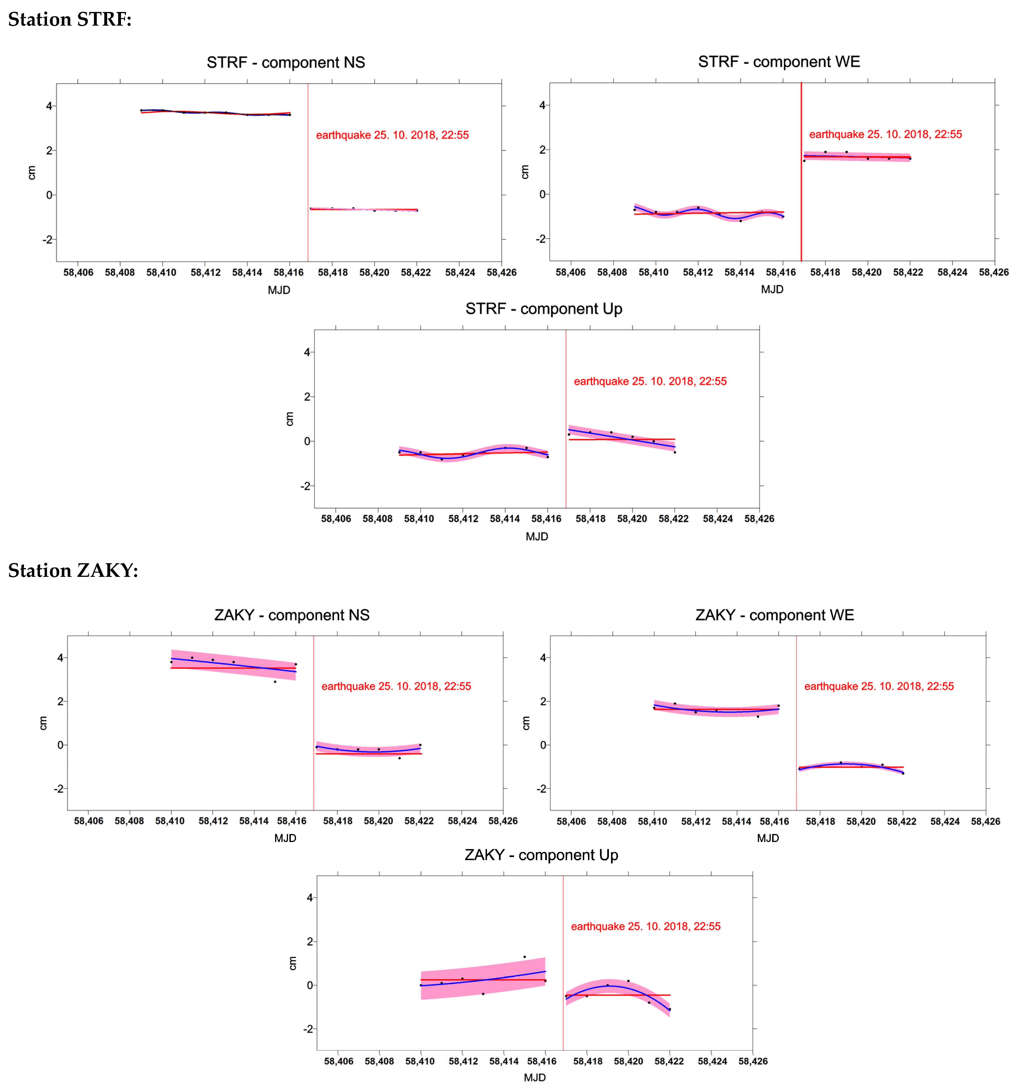
The detected co-seismic displacement at the EYPA station with an accuracy calculated using the 2nd approach RMSE is in decent agreement with the static displacement calculated from the seismic model (see Table 1). In the case of stations in the Zakynthos area, the 2nd approach for RMSE shows that the Up component of the co-seismic displacement cannot be a reliably determined. The 2.95 sigma errors (1.12, 2.21, 1.65 cm for the STRF, ZAKY, and PYRG stations, respectively) are larger than the absolute values of the Up components of the co-seismic displacements (0.66, 0.70, 0.35 cm for the STRF, ZAKY and PYRG stations, respectively—see also Table 2). Therefore, the 2nd approach of calculating RMSE gives better information about the accuracy of the detected co-seismic displacement and more credibly assess the significance of the determined co-seismic displacement than the RMSE of the 1st approach, which is unrealistically small.

In summary:

• A one-day solution using the PPP method give sufficient accuracy for further analysis.
• Anharmonic spectral analysis of a coordinate time series, in some cases, gives a more reliable estimate of co-seismic displacement than the difference of arithmetic averages of coordinates before and after a seismic event.
• In the 2nd approach, RMSE determines the dispersion of the approximation data from the time series analysis before and after the earthquake event.
• The RMSE from the 2nd approach gives a more realistic estimate of accuracy of co-seismic displacement than the RMSE from the 1st approach.

The aim of this study was to determine the co-seismic displacement from the GNSS data and to best estimate the accuracy of its determination. The use of the PPP method offers an advantage over the relative network solution in obtaining an “absolute” positional change for any given station. The disadvantage may be that the minimum length of the processed measurement, while achieving the required accuracy of the result, is one day. This precludes the possibility of determining co-seismic movements during an earthquake; however, we have shown that it is possible to determine co-seismic displacement. Any afterslips that occur within 1 day are included in the designated co-seismic displacement. An anharmonic spectral analysis was used to determine the difference in position before and after an earthquake from the time series of coordinates. In some cases, it has been shown to be a better method than the commonly used arithmetic average. Afterslips longer than 1 day are excluded using the anharmonic analysis. In our case studies, these only appeared in one component at the EYPA station. It has also been shown that the proposed 2nd approach to determine the RMSE of co-seismic displacement gives a more reliable estimate of accuracy than the 1st approach, which usually gives an unrealistically low estimate. The determination of the reliability of the resulting co-seismic displacement is higher and thus determined co-seismic displacement can be used in seismological interpretations and geokinematic studies. This is also important from an inter-disciplinary point of view, where the results of geodetic methods using GNSS are used by experts from other research branches. It is not only the result itself, which is important, but also its accuracy.