
Automotive Body Shop Design Problems Using Meta-Models Considering Product-Mix Change and Reconfiguration Strategy


Abstract
1. Introduction
2. Related Topics and Literatures
2.1. Automotive Body Shop Design
2.2. Performance Evaluating Methods for Manufacturing System Design
2.2.1. Stochastic Modeling
2.2.2. Simulation
2.2.3. Meta-Modeling
2.3. Buffer Allocation Problem (BAP)
3. System Configurations
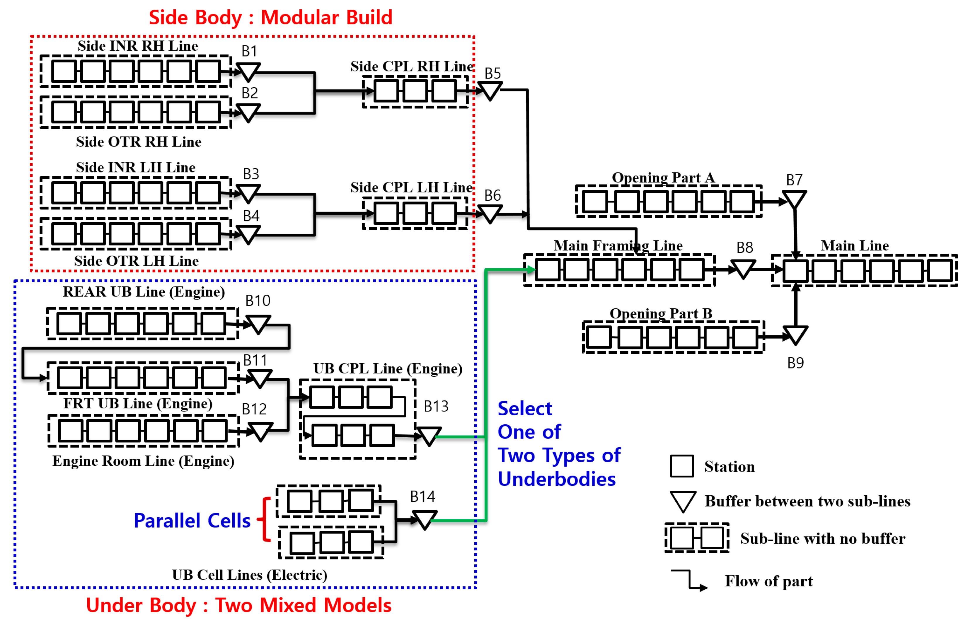
3.1. Basic Configuration
- Both the engine and electric cars are produced for the same car model. The total target production volume is fixed, but the individual production volume can be changed according to the product mix.
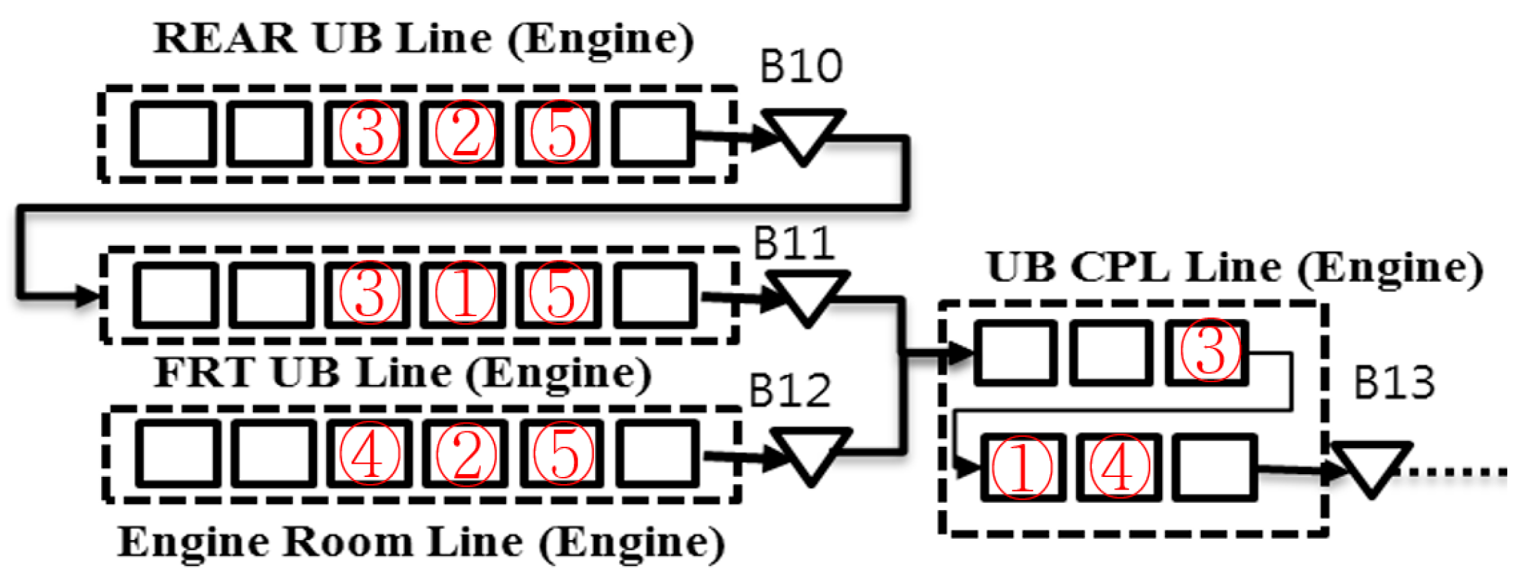
- All sublines except for the underbody lines are typically shared. However, two types of underbody lines exist: one for the engine car and the other for the electric car. The layout of the underbody lines for the engine car is similar to the traditional layout. However, the structure of underbody lines for the electric car is designed based on the concept of a cell system owing to the low production volume. When the production volume of the electric car increases, we can install additional cell lines in parallel.
- Buffers exist between two sublines (total number of buffer locations is 14); however, no buffer exists between two successive stations in a subline.
- The process times (PT) of all stations in sublines for the upper body (side body and main body) and the opening parts are constant and known as one time unit (minute) because a body shop is a highly automated manufacturing system.
- The PTs of the underbody lines (cells) can be changed according to the change in the product mix of two types of cars. The total workload is fixed; hence, the process time of a workstation is determined by the number of work stations. We assume that a perfect line balancing is possible.
- Only one mode of time-dependent failure exists for all workstations, and the distributions of time-to-failure (uptime) and time-to-repair (downtime) are exponentially distributed.
- No starvation occurs in the first stations, and no blocking occurs in the final stations. The first stations denote stations without predecessors, whereas the final stations are stations without successors.
3.2. Reconfiguration Strategies
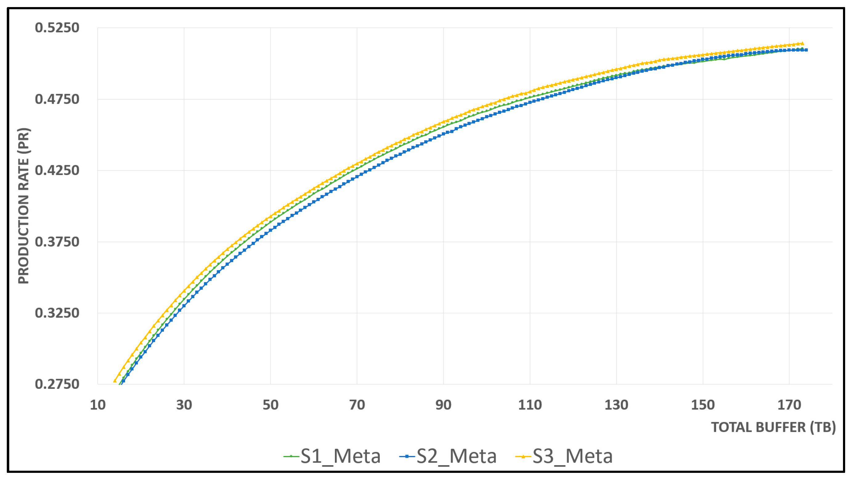
3.2.1. Strategy 1
3.2.2. Strategy 2
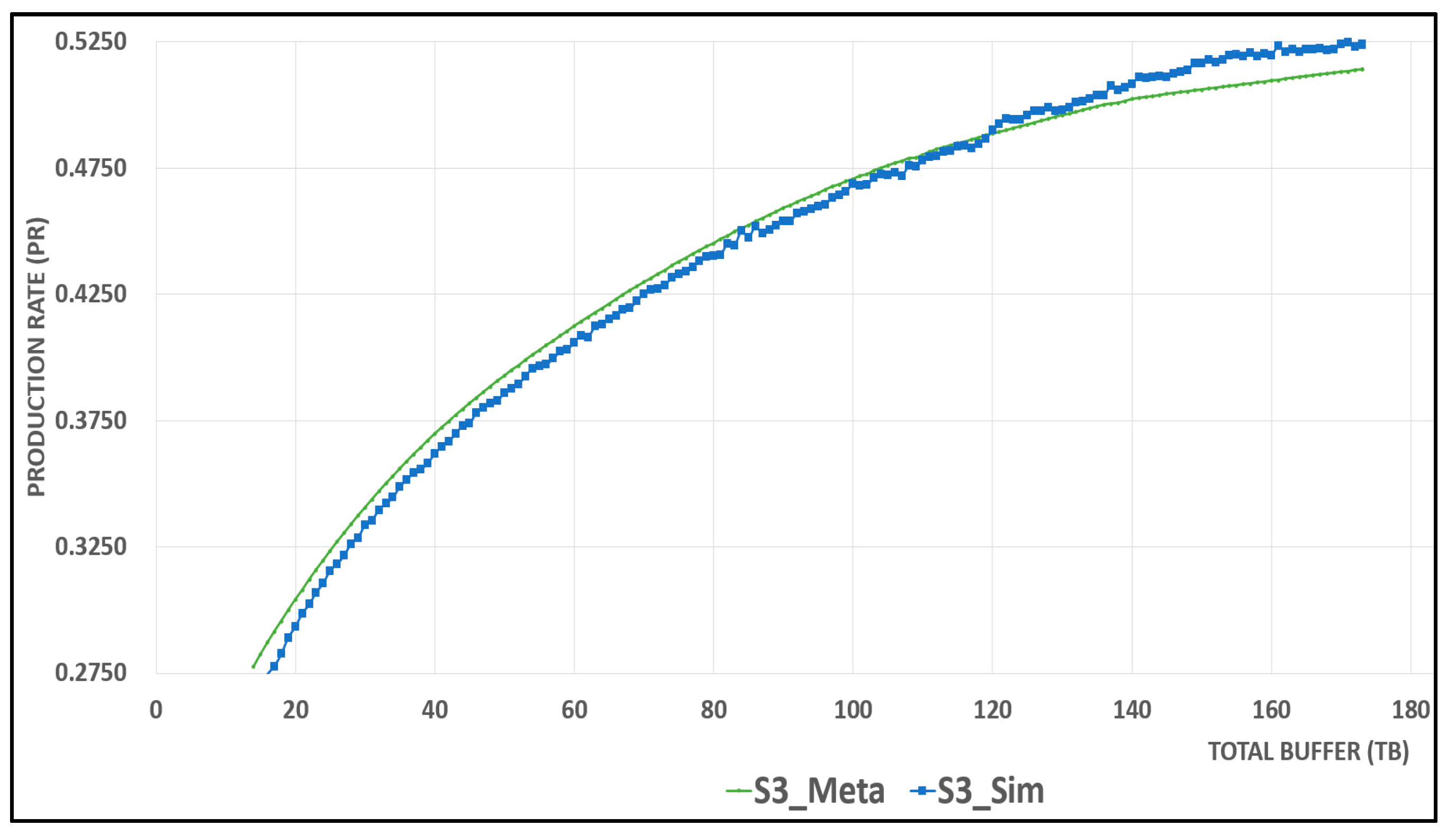
3.2.3. Strategy 3
4. Procedure of Meta-Modeling
4.1. Shape Determination of Meta-Model
4.2. Grouping Input Variables
- 14 buffers between two sublines (–)
- Isolated efficiency of each station
- Mean time to failure
- Product mix of two car models
- Process time of electric car
4.3. Design of Experiments
4.4. Determination of the Meta-Model
4.5. Validation of Meta-Model
5. Application to Manufacturing System Design Problems
5.1. Production Rate Maximization Problem
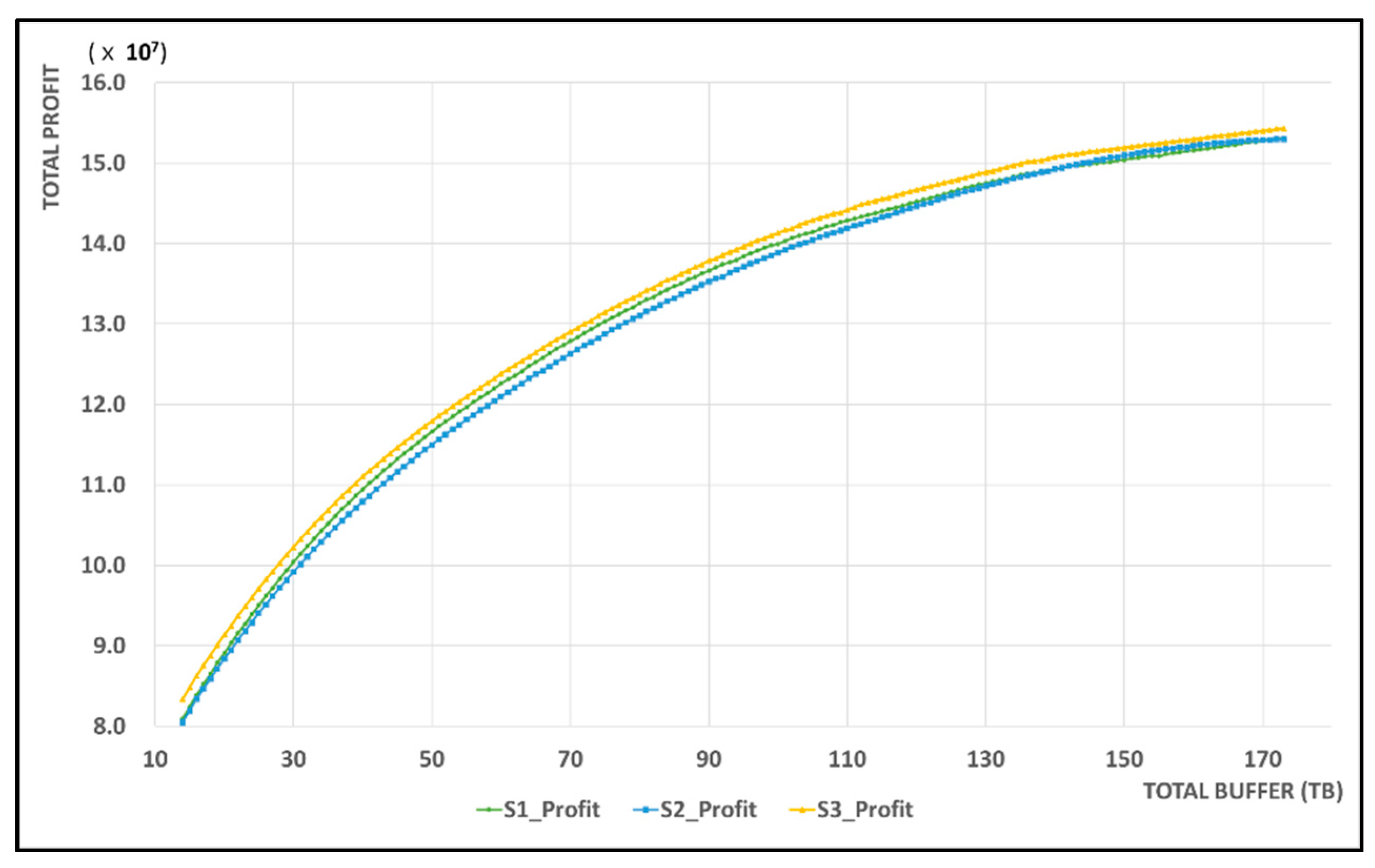
5.2. Profit Maximization Problem
6. Conclusions
Author Contributions
Funding
Institutional Review Board Statement
Informed Consent Statement
Data Availability Statement
Conflicts of Interest
References
- Omar, M.A. The Automotive Body Manufacturing Systems and Processes; John Wiley & Sons: New York, NY, USA, 2011. [Google Scholar]
- Naitoh, T.; Yamamoto, K.; Kodama, Y.; Honda, S. The Development of an Intelligent Body Assembly System. In Transforming Automobile Assembly; Shimokawa, S., Jürgens, U., Fujimoto, T., Eds.; Springer: Berlin/Heidelberg, Germany, 1997; pp. 121–132. [Google Scholar]
- Rooks, B. Rover 75 sets new standards in body-in-white assembly. Ind. Rob. 1999, 26, 342–348. [Google Scholar] [CrossRef]
- Moon, D.H.; Cho, H.I.; Kim, H.S.; Sunwoo, H.; Jung, J.Y. A case study of the body shop design in an automotive factory using 3D simulation. Int. J. Prod. Res. 2006, 44, 4121–4135. [Google Scholar] [CrossRef]
- Hansen, J.O.; Kampker, A.; Triebs, J. Approaches for flexibility in the future automobile body shop: Results of a comprehensive cross-industry study. Procedia CIRP 2018, 72, 995–1002. [Google Scholar] [CrossRef]
- Giampieri, A.; Ling-Chin, J.; Ma, Z.; Smallbone, A.; Roskilly, A.P. A review of the current automotive manufacturing practice from an energy perspective. Appl. Energy 2020, 261, 114074. [Google Scholar] [CrossRef]
- Frieske, B.; Kloetzke, M.; Mauser, F. Trends in vehicle concept and key technology development for hybrid and battery electric vehicles. In 2013 World Electric Vehicle Symposium and Exhibition (EVS27); IEEE: Barcelona, Spain, 2013; pp. 1–12. [Google Scholar] [CrossRef]
- Casper, R.; Sundin, E. Electrification in the automotive industry: Effects in remanufacturing. J. Remanuf. 2020. [Google Scholar] [CrossRef]
- Koren, Y.; Heisel, U.; Jovane, F.; Moriwaki, T.; Pritschow, G.; Ulsoy, G.; Van Brussel, H. Reconfigurable manufacturing systems. CIRP Ann. Manuf. Technol. 1999, 48, 527–540. [Google Scholar] [CrossRef]
- Koren, Y.; General, R.M.S. characteristics. Comparison with dedicated and flexible systems. In Reconfigurable Manufacturing Systems and Transformable Factories; Dashchenko, A.I., Ed.; Springer: Berlin/Heidelberg, Germany, 2006; pp. 27–45. [Google Scholar] [CrossRef]
- Bortolini, M.; Galizia, F.G.; Mora, C. Reconfigurable manufacturing systems: Literature review and research trend. J. Manuf. Syst. 2018, 49, 93–106. [Google Scholar] [CrossRef]
- Moon, D.H.; Kim, D.O.; Lee, Y.H.; Shin, Y.W. A simulation study on the effect of reconfiguration strategy in an automotive body shop considering the change of product-mix. In Proceedings of the 9th International Conference on Operations Research and Enterprise Systems (ICORES 2020), Valletta, Malta, 22–24 February 2020; pp. 430–435. [Google Scholar] [CrossRef]
- Muhl, E.; Charpentier, P.; Chaxel, F. Optimization of physical flows in an automotive manufacturing plant: Some experiments and issues. Eng. Appl. Artif. Intell. 2003, 16, 293–305. [Google Scholar] [CrossRef]
- Tahar, R.B.M.; Adham, A.A.J. Design and analysis of automobiles manufacturing system based on simulation model. Mod. Appl. Sci. 2010, 4, 130–134. [Google Scholar] [CrossRef][Green Version]
- Spieckermann, S.; Gutenschwager, K.; Heinzel, H.; Voß, S. Simulation-based optimization in the automotive industry—A case study on body shop design. Simulation 2000, 75, 276–286. [Google Scholar]
- Feno, M.R.; Cauvin, A.; Ferrarini, A. Conceptual design and simulation of an automotive body shop assembly line. IFAC Proc. Vol. 2014, 47, 760–765. [Google Scholar] [CrossRef]
- Kim, H.S.; Wang, G.; Shin, Y.W.; Moon, D.H. Comparison of the two layout structures in automotive body shops considering failure distributions. J. Korean Inst. Ind. Eng. 2015, 41, 470–480. [Google Scholar] [CrossRef][Green Version]
- Moon, D.H.; Nam, Y.S.; Kim, H.S.; Shin, Y.W. Effect of part transfer policies in two types of layouts in automotive body shops. Int. J. Ind. Eng. Theory 2017, 24, 194–206. [Google Scholar]
- Moon, D.H.; Nam, Y.S.; Shin, Y.W. Effects of additional sub-lines and buffer allocation on the system performance in an automotive body shop. J. Korean Soc. Supply Chain Manag. 2016, 16, 135–145. [Google Scholar]
- Moon, D.H.; Lee, Y.H.; Shin, Y.W. The effect of mixed-model production in automotive body shops considering assembly methods and part transfer policies. J. Korean Inst. Ind. Eng. 2018, 44, 391–403. [Google Scholar] [CrossRef]
- Kahan, T.; Bukchin, Y.; Menassa, R.; Ben-Gal, I. Backup strategy for robots’ failures in an automotive assembly system. Int. J. Prod. Econ. 2009, 120, 315–326. [Google Scholar] [CrossRef][Green Version]
- Azzi, A.; Battini, D.; Faccio, M.; Persona, A. Mixed model assembly system with multiple secondary feeder lines: Layout design and balancing procedure for ATO environment. Int. J. Prod. Res. 2012, 50, 5132–5151. [Google Scholar] [CrossRef]
- Azzi, A.; Battini, D.; Faccio, M.; Persona, A. Sequencing procedure for balancing the workloads variations in case of mixed model assembly system with multiple secondary feeder lines. Int. J. Prod. Res. 2012, 50, 6081–6098. [Google Scholar] [CrossRef]
- Faccio, M.; Bottin, M.; Rosati, G. Collaborative and traditional robotic assembly: A comparison model. Int. J. Adv. Manuf. Technol. 2019, 102, 1355–1372. [Google Scholar] [CrossRef]
- Gershwin, S.B. Manufacturing System Engineering; Prentice-Hall International: London, UK, 1994. [Google Scholar]
- Li, J.S.; Meerkov, S.M. Production Systems Engineering; Springer: New York, NY, USA, 2009. [Google Scholar]
- Dallery, Y.; Gershwin, S.B. Manufacturing flow line systems: A review of models and analytical results. Queueing Syst. 1992, 12, 3–94. [Google Scholar] [CrossRef]
- Papadopoulos, H.T.; Heavey, C. Queueing theory in manufacturing systems analysis and design: A classification of models for production and transfer lines. Eur. J. Oper. Res. 1996, 92, 1–27. [Google Scholar] [CrossRef]
- Altiok, T. Performance Analysis of Manufacturing Systems; Springer: New York, NY, USA, 1997. [Google Scholar]
- Li, J.S.; Blumenfeld, D.E.; Huang, N.; Alden, J.M. Throughput analysis of production systems: Recent advances and future topics. Int. J. Prod. Res. 2009, 47, 3823–3851. [Google Scholar] [CrossRef]
- Papadopoulos, C.T.; Li, J.; O’Kelly, M.E.J. A classification and review of timed Markov models of manufacturing systems. Comput. Ind. Eng. 2019, 128, 219–244. [Google Scholar] [CrossRef]
- Tancrez, J.S. A decomposition method for assembly/disassembly systems with blocking and general distributions. Flex. Serv. Manuf. J. 2020, 32, 272–296. [Google Scholar] [CrossRef]
- Cohen, Y.; Faccio, M.; Pilati, F.; Tao, X. Design and management of digital manufacturing and assembly systems in the Industry 4.0 era. J. Adv. Manuf. Technol. 2019, 105, 3565–3577. [Google Scholar] [CrossRef]
- Kleijnen, J.P.C. Kriging metamodeling in simulation: A review. Eur. J. Oper. Res. 2009, 192, 707–716. [Google Scholar] [CrossRef]
- Can, B.; Heavey, C. Comparison of experimental designs for simulation-based symbolic regression of manufacturing systems. Comput. Ind. Eng. 2011, 61, 447–462. [Google Scholar] [CrossRef]
- Kleijnen, J.P.C.; Standridge, C.R. Experimental design and regression analysis in simulation: An FMS case study. Eur. J. Oper. Res. 1988, 33, 257–261. [Google Scholar] [CrossRef][Green Version]
- Durieux, S.; Pierreval, H. Regression metamodeling for the design of automated manufacturing system composed of parallel machines sharing a material handling resource. Int. J. Prod. Econ. 2004, 89, 21–30. [Google Scholar] [CrossRef]
- Motlagh, M.M.; Azimi, P.; Amiri, M.; Madraki, G. An efficient simulation Optimization methodology to solve a multi-objective problem in unreliable unbalanced production lines. Expert Syst. Appl. 2019, 138, 112836. [Google Scholar] [CrossRef]
- Dengiz, B.; Akbay, K.S. Computer simulation of a PCB production line: Meta-modeling approach. Int. J. Prod. Econ. 2000, 63, 195–205. [Google Scholar] [CrossRef]
- Um, I.S.; Cheon, H.J.; Lee, H.C. The simulation design and analysis of a flexible manufacturing system with automated guided vehicle system. J. Manuf. Sys. 2009, 28, 115–122. [Google Scholar] [CrossRef]
- Dengiz, B.; Tansel, İ.; Belgin, O. A meta-model based simulation optimization using hybrid simulation-analytical modeling to increase the productivity in automotive industry. Math. Comput. Simulat. 2016, 120, 120–128. [Google Scholar] [CrossRef]
- Weiss, S.; Schwarz, J.A.; Stolletz, R. The buffer allocation problem in production lines: Formulations, solution methods, and instances. IISE Trans. 2019, 51, 456–485. [Google Scholar] [CrossRef]
- Chan, F.T.S.; Ng, E.Y.H. Comparative evaluations of buffer allocation strategies in a serial production line. Int. J. Adv. Manuf. Technol. 2002, 19, 789–800. [Google Scholar] [CrossRef]
- Amiri, M.; Mohtashami, A. Buffer allocation in unreliable production lines based on design of experiments, simulation, and genetic algorithm. Int. J. Adv. Manuf. Technol. 2012, 62, 371–383. [Google Scholar] [CrossRef]
- Papadopoulos, C.T.; O’Kelly, M.E.J.; Tsadiras, A.K. A DSS for the buffer allocation of production lines based on a comparative evaluation of a set of search algorithms. Int. J. Prod. Res. 2013, 51, 4175–4199. [Google Scholar] [CrossRef]
- Demir, L.; Tunali, S.; Eliiyi, D.T. The state of the art on buffer allocation problem: A comprehensive survey. J. Intell. Manuf. 2014, 25, 371–392. [Google Scholar] [CrossRef]
- Liberopoulos, G. Comparison of optimal buffer allocation in flow lines under installation buffer, echelon buffer, and CONWIP policies. Flex. Serv. Manuf. J. 2020, 32, 297–365. [Google Scholar] [CrossRef]
- Bezerra, M.A.; Santelli, R.E.; Oliveira, E.P.; Villar, L.S.; Escaleira, L.A. Response surface methodology (RSM) as a tool for optimization in analytical chemistry. Talanta 2008, 76, 965–977. [Google Scholar] [CrossRef]
- Grömping, U. R package DoE.base for factorial experiments. J. Stat. Softw. 2018, 85, 1–41. [Google Scholar] [CrossRef]
- Groemping, U.; John, F. Package ‘RcmdrPlugin.DoE’ (R Package Version 0.12-3). 2014. Available online: https://cran.r-project.org/web/packages/RcmdrPlugin.DoE/index.html (accessed on 20 August 2020).
- Pérez, M.E.; Pericchi, L.R. Changing statistical significance with the amount of information: The adaptive α significance level. Stat. Probab. Lett. 2014, 85, 20–24. [Google Scholar] [CrossRef] [PubMed]
- Liberopoulos, G. Performance evaluation of a production line operated under an echelon buffer policy. IISE Trans. 2018, 50, 161–177. [Google Scholar] [CrossRef]


| References | Manufac. Sys. Types | Products | Performances | Performance Analysis Methods | Objectives | |
|---|---|---|---|---|---|---|
| Sim. | Meta | |||||
| Spieckermann [15] | AL(FABS) | Single | PR, CT | ● | Min. Cost | |
| Kahan [21] | AL(PABS) | Single | CT | ● | Comp. | |
| Feno [16] | AL(PABS) | Multiple | CT, TP | ● | Comp. | |
| Kim [17] | AL(PABS) | Single | PR | ● | Comp. | |
| Moon [4] | AL(FABS) | Single | TP | ● | Max. TP | |
| Moon [18] | AL(PABS) | Single | PR, LT | ● | Comp. | |
| Moon [19] | AL(PABS) | Single | PR, LT | ● | Max. PR | |
| Moon [20] | AL(PABS) | Multiple | PR, LT | ● | Comp. | |
| Can [35] | FL | Single | TR | ● | Max TP | |
| Dengiz [39] | FL | Single | PR, CT | ● | Comp. | |
| Motlagh [38] | FLP | Multiple | TP, WIP, | ● | Multi. | |
| Dengiz [41] | FLR | Multiple | TP | ● | Max. TP | |
| Kleijnen [36] | FMS | Single | TP | Max TP | ||
| Durieux [37] | FMS | Multiple | Util. | ● | - | |
| Um [40] | FMS | Multiple | TP, AGV Util. etc. | ● | Multi. | |
| This paper | AL(FABS) | Multiple | PR | ● | Max. PR, Max. Profit | |
| Engine Car (Type 1) | Electric Car (Type 2) | |
|---|---|---|
| 24 | 21 | |
| 24 | 3 | |
| 1 | 7 |
| Electric Car (Type 2) | Engine Car (Type 1) | ||||
|---|---|---|---|---|---|
| Product-Mix | Number of Cell Lines | Strategy 1 | Strategies 2 and 3 | ||
| NS1 | PT1 | NS1 | PT1 | ||
| 0% | 0 | 24 | 1.0 | 24 | 1.0000 |
| 10% | 1 | 24 | 1.0 | 22 | 1.0909 |
| 20% | 2 | 24 | 1.0 | 20 | 1.2000 |
| 30% | 3 | 24 | 1.0 | 17 | 1.4118 |
| 40% | 4 | 24 | 1.0 | 15 | 1.6000 |
| 50% | 5 | 24 | 1.0 | 12 | 2.0000 |
| Input Variables | Range of Levels (α = 2) | |||||
|---|---|---|---|---|---|---|
| Notation | Definition | Min | Low | Medium | High | Max |
| Buffer capacity of group 1 (, ) | 1 | 4 | 7 | 10 | 13 | |
| Buffer capacity of group 2 () | 1 | 4 | 7 | 10 | 13 | |
| Buffer capacity of group 3 () | 1 | 4 | 7 | 10 | 13 | |
| Buffer capacity of group 4 () | 1 | 4 | 7 | 10 | 13 | |
| Buffer capacity of group 5 () | 1 | 4 | 7 | 10 | 13 | |
| Buffer capacity of group 6 () | 1 | 4 | 7 | 10 | 13 | |
| Buffer capacity of group 7 () | 1 | 4 | 7 | 10 | 13 | |
| Buffer capacity of group 8 () | 1 | 2 | 3 | 4 | 5 | |
| Efficiency of each station (e) | 0.94 | 0.95 | 0.96 | 0.97 | 0.98 | |
| Mean time to failure (1/f) | 160 | 200 | 240 | 280 | 320 | |
| Product mix | 0.1 | 0.2 | 0.3 | 0.4 | 0.5 | |
| The process time of each station for electric cars ( | 5.6 | 6.2 | 6.8 | 7.4 | 8 | |
| Data Set | Original Levels | Normalized Levels | |||||||||||||||||||||||
|---|---|---|---|---|---|---|---|---|---|---|---|---|---|---|---|---|---|---|---|---|---|---|---|---|---|
| 1 | 4 | 4 | 4 | 4 | 4 | 4 | 4 | 2 | 0.95 | 200 | 0.2 | 6.2 | −1 | −1 | −1 | −1 | −1 | −1 | −1 | −1 | −1 | −1 | −1 | −1 | 0.2973 |
| 2 | 10 | 4 | 4 | 4 | 4 | 4 | 4 | 2 | 0.97 | 280 | 0.4 | 7.4 | 1 | −1 | −1 | −1 | −1 | −1 | −1 | −1 | 1 | 1 | 1 | 1 | 0.5001 |
| : | |||||||||||||||||||||||||
| 255 | 4 | 10 | 10 | 10 | 10 | 10 | 10 | 4 | 0.95 | 200 | 0.2 | 6.2 | −1 | 1 | 1 | 1 | 1 | 1 | 1 | 1 | −1 | −1 | −1 | −1 | 0.3830 |
| 256 | 10 | 10 | 10 | 10 | 10 | 10 | 10 | 4 | 0.97 | 280 | 0.4 | 7.4 | 1 | 1 | 1 | 1 | 1 | 1 | 1 | 1 | 1 | 1 | 1 | 1 | 0.5867 |
| 257 | 1 | 7 | 7 | 7 | 7 | 7 | 7 | 3 | 0.96 | 240 | 0.3 | 6.8 | −2 | 0 | 0 | 0 | 0 | 0 | 0 | 0 | 0 | 0 | 0 | 0 | |
| 258: | 13 | 7 | 7 | 7 | 7 | 7 | 7 | 3 | 0.96 | 240 | 0.3 | 3.8 | 2 | 0 | 0 | 0 | 0 | 0 | 0 | 0 | 0 | 0 | 0 | 0 | |
| : | |||||||||||||||||||||||||
| 279 | 7 | 7 | 7 | 7 | 7 | 7 | 7 | 3 | 0.96 | 240 | 0.3 | 5.6 | 0 | 0 | 0 | 0 | 0 | 0 | 0 | 0 | 0 | 0 | 0 | −2 | 0.4344 |
| 280 | 7 | 7 | 7 | 7 | 7 | 7 | 7 | 3 | 0.96 | 240 | 0.3 | 8 | 0 | 0 | 0 | 0 | 0 | 0 | 0 | 0 | 0 | 0 | 0 | 2 | 0.4336 |
| 281 | 7 | 7 | 7 | 7 | 7 | 7 | 7 | 3 | 0.96 | 240 | 0.3 | 6.8 | 0 | 0 | 0 | 0 | 0 | 0 | 0 | 0 | 0 | 0 | 0 | 0 | 0.4349 |
| : | |||||||||||||||||||||||||
| 288 | 7 | 7 | 7 | 7 | 7 | 7 | 7 | 3 | 0.96 | 240 | 0.3 | 6.8 | 0 | 0 | 0 | 0 | 0 | 0 | 0 | 0 | 0 | 0 | 0 | 0 | 0.4349 |
| Term | Coef. | SE Coef. | t | p | Term | Coef. | SE Coef. | t | p |
|---|---|---|---|---|---|---|---|---|---|
| Const. | 0.4340 | 0.0004 | 1070.01 | <0.001 | 0.0005 | 0.0001 | 4.07 | <0.001 | |
| 0.0160 | 0.0001 | 143.57 | <0.001 | 0.0009 | 0.0001 | 8.01 | <0.001 | ||
| 0.0152 | 0.0001 | 136.60 | <0.001 | −0.0003 | 0.0001 | −2.51 | <0.002 | ||
| 0.0103 | 0.0001 | 92.03 | <0.001 | 0.0011 | 0.0001 | 9.38 | <0.001 | ||
| 0.0095 | 0.0001 | 85.42 | <0.001 | 0.0007 | 0.0001 | 5.90 | <0.001 | ||
| 0.0018 | 0.0001 | 15.90 | <0.001 | 0.0002 | 0.0001 | 2.07 | <0.04 | ||
| 0.0014 | 0.0001 | 12.99 | <0.001 | 0.0002 | 0.0001 | 2.06 | <0.04 | ||
| 0.0045 | 0.0001 | 40.57 | <0.001 | 0.0006 | 0.0001 | 5.17 | <0.03 | ||
| 0.0003 | 0.0001 | 2.89 | <0.002 | −0.0002 | 0.0001 | −2.00 | <0.05 | ||
| 0.1066 | 0.0001 | 956.30 | <0.001 | 0.0007 | 0.0001 | 6.14 | <0.03 | ||
| −0.0277 | 0.0001 | −248.76 | <0.001 | −0.0010 | 0.0001 | −9.21 | <0.001 | ||
| 0.0069 | 0.0001 | 62.28 | <0.001 | 0.0003 | 0.0001 | 2.99 | <0.001 | ||
| −0.0002 | 0.0001 | −1.68 | 0.094 | 0.0006 | 0.0001 | 5.68 | <0.001 | ||
| −0.0031 | 0.0003 | −10.18 | <0.001 | −0.0005 | 0.0001 | −4.31 | <0.001 | ||
| −0.0023 | 0.0003 | −7.52 | <0.001 | 0.0007 | 0.0001 | 6.17 | <0.001 | ||
| −0.0020 | 0.0003 | −6.70 | <0.001 | 0.0005 | 0.0001 | 4.40 | <0.001 | ||
| −0.0012 | 0.0003 | −3.84 | <0.001 | −0.0002 | 0.0001 | −2.01 | <0.05 | ||
| −0.0015 | 0.0003 | −4.80 | <0.001 | 0.0004 | 0.0001 | 3.46 | <0.001 | ||
| 0.0142 | 0.0003 | 46.69 | <0.001 | −0.0002 | 0.0001 | −2.14 | <0.04 | ||
| 0.0027 | 0.0003 | 8.97 | <0.001 | −0.0003 | 0.0001 | −2.36 | <0.001 | ||
| −0.0010 | 0.0003 | −3.29 | <0.004 | −0.0009 | 0.0001 | −8.16 | <0.02 | ||
| −0.0020 | 0.0001 | −17.72 | <0.001 | −0.0004 | 0.0001 | −3.26 | <0.001 | ||
| 0.0012 | 0.0001 | 10.81 | <0.001 | −0.0009 | 0.0001 | −7.96 | <0.001 | ||
| 0.0005 | 0.0001 | 4.81 | <0.001 | 0.0003 | 0.0001 | 2.77 | <0.001 | ||
| 0.0004 | 0.0001 | 3.42 | <0.001 | −0.0018 | 0.0001 | −15.51 | <0.001 | ||
| 0.0003 | 0.0001 | 2.69 | <0.01 | 0.0007 | 0.0001 | 5.98 | <0.001 |
| Data Set | DF | Adj. SS | F | p | |
|---|---|---|---|---|---|
| Model | Linear | 12 | 3.4030 | 86,449 | <0.001 |
| Quadratic | 8 | 0.0079 | 302.15 | <0.001 | |
| 2 way interaction | 31 | 0.0044 | 45.56 | <0.001 | |
| Total model | 51 | 3.4153 | 2671.62 | <0.001 | |
| Residual | Lack of fit | 230 | 0.0008 | 1.1436 × | <0.001 |
| Pure error | 6 | 0 | |||
| Total error | 236 | 0.0008 | |||
| R-square (Adj.) = 99.98 | |||||
| Data Set | Number of Points | APE (%) | |||
|---|---|---|---|---|---|
| Minimum | Mean | Maximum | |||
| DOE points | 288 | 0.00 | 0.29 | 2.91 | |
| Random points | = 1 | 45 | 0.00 | 0.21 | 0.57 |
| = 2 | 45 | 0.03 | 1.01 | 5.16 | |
| TB | Optimal Buffer Allocation | PRmeta | PRsim | APE (%) | |||||||
|---|---|---|---|---|---|---|---|---|---|---|---|
| z1 (4) | z2 (2) | z3 (2) | z4 (1) | z5 (2) | z6 (1) | z7 (1) | z8 (1) | ||||
| 14 | 1 | 1 | 1 | 1 | 1 | 1 | 1 | 1 | 0.2775 | 0.2625 | −5.70 |
| 15 | 1 | 1 | 1 | 2 | 1 | 1 | 1 | 1 | 0.2825 | 0.2693 | −4.90 |
| 18 | 1 | 1 | 1 | 5 | 1 | 1 | 1 | 1 | 0.2957 | 0.2827 | −4.61 |
| 19 | 1 | 2 | 1 | 4 | 1 | 1 | 1 | 1 | 0.3000 | 0.2892 | −3.72 |
| 20 | 1 | 2 | 1 | 5 | 1 | 1 | 1 | 1 | 0.3041 | 0.2933 | −3.75 |
| 21 | 1 | 3 | 1 | 4 | 1 | 1 | 1 | 1 | 0.3079 | 0.2987 | −3.11 |
| 29 | 1 | 5 | 1 | 8 | 1 | 1 | 1 | 1 | 0.3374 | 0.3285 | −2.68 |
| 30 | 1 | 5 | 1 | 8 | 1 | 1 | 2 | 1 | 0.3405 | 0.3336 | −2.07 |
| 40 | 1 | 8 | 1 | 11 | 1 | 1 | 3 | 1 | 0.3697 | 0.3620 | −2.13 |
| 50 | 1 | 10 | 2 | 13 | 1 | 1 | 5 | 1 | 0.3927 | 0.3861 | −1.71 |
| 56 | 1 | 11 | 4 | 12 | 1 | 1 | 6 | 1 | 0.4048 | 0.3973 | −1.90 |
| 57 | 1 | 11 | 4 | 12 | 1 | 1 | 7 | 1 | 0.4065 | 0.3995 | −1.74 |
| 58 | 2 | 10 | 4 | 12 | 1 | 1 | 6 | 1 | 0.4085 | 0.4023 | −1.55 |
| 59 | 2 | 11 | 3 | 13 | 1 | 1 | 6 | 1 | 0.4104 | 0.4030 | −1.82 |
| 60 | 2 | 11 | 4 | 12 | 1 | 1 | 6 | 1 | 0.4124 | 0.4060 | −1.57 |
| 70 | 3 | 12 | 5 | 13 | 1 | 1 | 7 | 1 | 0.4298 | 0.4251 | −1.10 |
| 80 | 5 | 12 | 6 | 13 | 1 | 1 | 7 | 1 | 0.4451 | 0.4402 | −1.12 |
| 90 | 6 | 12 | 8 | 13 | 1 | 1 | 9 | 1 | 0.4592 | 0.4539 | −1.18 |
| 100 | 7 | 13 | 9 | 13 | 1 | 1 | 11 | 1 | 0.4706 | 0.4688 | −0.86 |
| 110 | 8 | 13 | 12 | 13 | 1 | 1 | 11 | 1 | 0.4803 | 0.4780 | −0.48 |
| 120 | 10 | 13 | 12 | 13 | 1 | 2 | 12 | 1 | 0.4886 | 0.4902 | 0.33 |
| 130 | 10 | 13 | 12 | 13 | 1 | 13 | 11 | 1 | 0.4959 | 0.4980 | 0.42 |
| 140 | 12 | 13 | 13 | 13 | 1 | 13 | 11 | 1 | 0.5023 | 0.5083 | 1.17 |
| 150 | 13 | 13 | 13 | 13 | 3 | 13 | 12 | 2 | 0.5061 | 0.5165 | 2.01 |
| 160 | 13 | 13 | 13 | 13 | 9 | 13 | 11 | 2 | 0.5096 | 0.5198 | 1.95 |
| 170 | 13 | 13 | 13 | 13 | 12 | 13 | 11 | 5 | 0.5131 | 0.5240 | 2.08 |
| 173 | 13 | 13 | 13 | 13 | 13 | 13 | 12 | 5 | 0.5140 | 0.5242 | 1.95 |
| Product-Mix | 20% | 30% | 40% | |||
|---|---|---|---|---|---|---|
| TB | (z1, …, z8) * | PR | (z1, …, z8) * | PR | (z1, …, z8) * | PR |
| 50 | (1,10,2,11,1,1,7,2) | 0.3825 | (1,10,2,13,1,1,5,1) | 0.3927 | (1,10,3,12,1,1,4,2) | 0.4023 |
| 70 | (3,11,5,13,1,1,9,1) | 0.4190 | (3,12,5,13,1,1,7,1) | 0.4298 | (3,12,6,13,1,1,5,1) | 0.4400 |
| 90 | (6,11,8,13,1,1,11,1) | 0.4475 | (6,12,8,13,1,1,9,1) | 0.4592 | (6,12,9,13,1,1,7,1) | 0.4700 |
| 110 | (9,12,10,13,1,1,13,1) | 0.4683 | (8,13,12,13,1,1,11,1) | 0.4807 | (9,13,11,13,1,1,9,1) | 0.4923 |
| 130 | (10,13,12,13,1,13,11,1) | 0.4859 | (10,13,12,13,1,13,11,1) | 0.4959 | (12,13,13,13,1,4,10,1) | 0.5062 |
| 150 | (12,13,13,13,5,13,13,1) | 0.4968 | (13,13,13,13,3,13,12,2) | 0.5061 | (13,13,13,13,2,13,10,5) | 0.5147 |
| TB | Strategy 1 | Strategy 2 | Strategy 3 | ||||||
|---|---|---|---|---|---|---|---|---|---|
| Using Meta-Model (Optimized) | Simulation | Using Meta-Model (Optimized) | Simulation | Using Meta-Model (Optimized) | Simulation | ||||
| TP (×108) | PR1 | 95% C.I. of PR1 | TP (×108) | PR2 | 95% C.I. of PR2 | TP (×108) | PR3 | 95% C.I. of PR3 | |
| 70 | 1.2789 | 0.4263 | 0.0013 | 1.2634 | 0.4205 | 0.0017 | 1.2907 | 0.4298 | 0.0020 |
| 90 | 1.3665 | 0.4555 | 0.0019 | 1.3529 | 0.4504 | 0.0009 | 1.3791 | 0.4592 | 0.0013 |
| 110 | 1.4287 | 0.4762 | 0.0016 | 1.4195 | 0.4725 | 0.0014 | 1.4422 | 0.4803 | 0.0016 |
| 130 | 1.4751 | 0.4917 | 0.0027 | 1.4719 | 0.4900 | 0.0015 | 1.4891 | 0.4959 | 0.0020 |
| 150 | 1.5042 | 0.5014 | 0.0013 | 1.5101 | 0.5028 | 0.0014 | 1.5196 | 0.5061 | 0.0018 |
Publisher’s Note: MDPI stays neutral with regard to jurisdictional claims in published maps and institutional affiliations. |
© 2021 by the authors. Licensee MDPI, Basel, Switzerland. This article is an open access article distributed under the terms and conditions of the Creative Commons Attribution (CC BY) license (http://creativecommons.org/licenses/by/4.0/).
Share and Cite
Moon, D.H.; Kim, D.O.; Shin, Y.W. Automotive Body Shop Design Problems Using Meta-Models Considering Product-Mix Change and Reconfiguration Strategy. Appl. Sci. 2021, 11, 2748. https://doi.org/10.3390/app11062748
Moon DH, Kim DO, Shin YW. Automotive Body Shop Design Problems Using Meta-Models Considering Product-Mix Change and Reconfiguration Strategy. Applied Sciences. 2021; 11(6):2748. https://doi.org/10.3390/app11062748
Chicago/Turabian StyleMoon, Dug Hee, Dong Ok Kim, and Yang Woo Shin. 2021. "Automotive Body Shop Design Problems Using Meta-Models Considering Product-Mix Change and Reconfiguration Strategy" Applied Sciences 11, no. 6: 2748. https://doi.org/10.3390/app11062748
APA StyleMoon, D. H., Kim, D. O., & Shin, Y. W. (2021). Automotive Body Shop Design Problems Using Meta-Models Considering Product-Mix Change and Reconfiguration Strategy. Applied Sciences, 11(6), 2748. https://doi.org/10.3390/app11062748