Article

A Novel Load Forecasting Approach Based on Smart Meter Data Using Advance Preprocessing and Hybrid Deep Learning

1
Department of Energy Systems Engineering, Faculty of Technology, Firat University, Elazığ 23110, Turkey
2
Department of Electrical Engineering, College of Engineering, University of Hail, Hail 55476, Saudi Arabia
*
Author to whom correspondence should be addressed.
Appl. Sci. 2021, 11(6), 2742; https://doi.org/10.3390/app11062742
Submission received: 24 February 2021 / Revised: 14 March 2021 / Accepted: 16 March 2021 / Published: 18 March 2021
(This article belongs to the Special Issue Smart Energy Buildings of the Future)

Abstract

:
Short-term load forecasting models play a critical role in distribution companies in making effective decisions in their planning and scheduling for production and load balancing. Unlike aggregated load forecasting at the distribution level or substations, forecasting load profiles of many end-users at the customer-level, thanks to smart meters, is a complicated problem due to the high variability and uncertainty of load consumptions as well as customer privacy issues. In terms of customers’ short-term load forecasting, these models include a high level of nonlinearity between input data and output predictions, demanding more robustness, higher prediction accuracy, and generalizability. In this paper, we develop an advanced preprocessing technique coupled with a hybrid sequential learning-based energy forecasting model that employs a convolution neural network (CNN) and bidirectional long short-term memory (BLSTM) within a unified framework for accurate energy consumption prediction. The energy consumption outliers and feature clustering are extracted at the advanced preprocessing stage. The novel hybrid deep learning approach based on data features coding and decoding is implemented in the prediction stage. The proposed approach is tested and validated using real-world datasets in Turkey, and the results outperformed the traditional prediction models compared in this paper.

1. Introduction

Short-term load forecasting has a vital role in making fast and reliable decisions for distribution systems. Recent improvements in the smart grid, especially with the introduction of smart meters, have led to a significant increase in the amount of data. Analyzing these big data produced by smart meters and understanding diverse patterns of electricity consumption by customers can help to create more accurate load prediction models. Although these new opportunities have attracted the attention of distribution companies, many problems remain to be solved in the relevant literature. The increasing penetration of renewable energy sources, complex interactions between utility and customer, and time-varying load demand in the distribution grids adversely affect system stability [1]. To this end, developing a customer-based prediction model makes it necessary to direct short-term load forecasting applications from the distribution system level to the user level. However, adopting only customer-based approaches is not enough by itself to create the most accurate load estimation model. Weather, schedule of system maintenance and repair, seasonality, human behavior, and other external factors are also important issues to be taken into consideration in the prediction model [2].
Nowadays, daily energy consumption information of various customers is constantly shared with distribution companies thanks to advanced communication infrastructure and smart meters. This information is stored in local or cloud databases to be used in operational activities or online decision-making. In this way, users can benefit from an interactive platform that may result in stable electricity bills at a reasonable price while distribution companies can precisely determine the supply and demand ratio. Therefore, it is crucial for all distribution companies to integrate an efficient load-forecasting model and to extract beneficial features from customers’ big data [3].
To grasp the problem of short-term load forecasting adequately in customer-level loads at the smart grid, despite the various solutions that have been conducted in the literature using numerous methods including advanced deep learning (DL) algorithms based on either an individual customer level or substation level as in Section 2, it seems obvious these days to acquire bidirectional flow of electricity consumption data via smart meters from all customers in the smart grid. This problem framework defines the customary workflow processes in the planning and operation of electrical systems including demand response, load forecasting, and energy scheduling that can build interactive platforms. Therefore, the existing solutions lack the development of a prediction model that acquires big data from all customers and provides more accurate consumption prediction using a hybrid DL algorithm and preprocessing enhancement. To the best of the authors knowledge, this issue of using advanced preprocessing techniques coupled with hyrid DL algorithm has not been studied previously. This study proposes advanced preprocessing techniques for load profile clustering and a hybrid DL algorithm, which is convolution neural network (CNN)—bidirectional long short-term memory (BLSTM), for short-term load forecasting of real big data sets in Turkey.
Generally, load forecasting can be influenced by many factors such as time, weather, and the type of customer [4]. The three main types of load forecasting in terms of time horizon are short-term forecasting, mid-term forecasting, and long-term forecasting. Short-term load forecasting has been studied in the literature for a time interval ranging from an hour to a couple of weeks for different applications such as real-time control, energy transfer scheduling, economic dispatch, and demand response [4]. In this study, we investigate the short-term forecasting problem for potential demand response and real-time control applications for one-hour-ahead prediction applied by the utility company. As a result of the application of short-term forecasting at the distribution level, the utility company can benefit from precise prediction for short-term planning applications such as peak shifting and load scheduling. On the other side, consumers plan their energy consumption based on real-time responses from the utility in order to reduce their monthly bills.
The motivation of this work is to develop a prediction model using a hybrid DL algorithm enhanced with feature clustering to find the lowest prediction errors for load forecasting in smart grids at the customer level. The hybrid DL algorithm includes a one-dimentional (1-D) CNN emerged with BLSTM, and feature selection enhancement includes data preprocessing using density-based spatial clustering applications with noise (DBSCAN) algorithm to extract frequent patterns. This work contributes to the solution of precision load forecasting at the customer-level in smart grids by using the DBSCAN algorithm coupled with the CNN–BLSTM model to build a robust prediction model.
The contents of the paper are organized as follows: the literature review is firstly presented in Section 2. In Section 3, we formulate the load forecasting problem. In Section 4, we elaborate on the hybrid DL algorithms. Then, we reformulate the prediction problem and elaborate thet modeling set-up in Section 5. The prediction results are evaluated and discussed in Section 6. Finally, some conclusions and future work are presented in Section 7.

2. Literature Survey

Over the past decades, many approaches have been proposed for robust and accurate prediction of energy consumption and short-term load forecasting at the distribution- level [4,5,6,7], but there are limited studies for customers-level load forecasting. Cai et al. [8] compared traditional time-series model seasonal autoregressive-integrated moving average with exogenous inputs (SARIMAX) with recurrent neural networks (RNNs) and CNN models in the application of day-ahead building-level load forecasting. The authors reported a decrease in day-ahead multi-step forecasting error by 22.6% on average for cases with strong weather covariance compared to the SARIMAX model.
Yong et al. [9] proposed a short-term load forecasting method based on a similar day selection and long short-term memory (LSTM) network for buildings. In [10], a network-based short-term load forecasting utilized the LSTM algorithm for residential buildings. The authors applied wavelet decomposition and collaborative representation methods to obtain the feature vector extracted from lagged load variables. In [11], the authors proposed a model based on empirical mode decomposition (EMD) and LSTM network for estimating electricity demand at a specified time interval. Another similar study was conducted in [12] for the residential buildings dataset. The authors concluded that the LSTM-based RNN model performed better compared with simple RNN and gated recurrent unit (GRU)–RNN models for a single user with a one-minute resolution. However, the uncertainty issues involved in this granular scale result in mean absolute percentage error (MAPE) values that range between 24% and 59%. In [13], the proposed BLSTM network has some important advantages as the networks can learn from raw data due to not requiring the feature extraction process and are capable of maintaining the long-term dependencies in time series data. The generalized additive model (GAM) in [14] fills missing data by modeling the input data as a sum of splines. Additionally, another advantage of GAM is to obtain interpretable information about the data and the covariates. Another implementation of deep learning is presented in [15] for the purpose of electricity-theft detection. The proposed method consists of two different components named wide and deep CNN. While the deep CNN component identifies periodic features from the input 2-D electricity consumption data, the wide CNN component obtains useful features from 1-D electricity consumption data. Deep learning-based fault diagnostics/prognostics implementations in the induction machine’s bearings are one of the most important issues in the field of fault detection [13,16].
Considering hybridizing two DL models in [17], the authors implemented two different sequence-to-sequence (S2S) RNN methods on a building-level energy consumption dataset. For the first RNNs, GRU encodes the information, and the second is the LSTM model that sequentially generates the outputs using this information. The proposed method was tested for three different prediction length scenarios and compared with traditional DL algorithms. The MAPE results varied between 2.441% and 23.698% on average for all scenarios. Another hybrid DL method for gas consumption estimation was introduced in [18]. The proposed method is based on wavelet transform (WT), BLSTM, and genetic algorithm (GA). The proposed methods prediction performance was tested on different horizons such as 1 h, 5 h, and 10 h, and the mean absolute error (MAE) values were 10.27, 11.96, and 55.11, respectively. Lastly, data imputation methods based on transfer learning and deep learning were studied in [19,20].

3. Preprocessing Methods

The problem of load forecasting at the customer level in a smart grid using energy consumption is a complex time-series problem. In this paper, we solve the time-series challenge by implementing a hybrid DL approach enhanced with advanced preprocessing techniques to solve complex systems and to reduce prediction errors. Therefore, the modeling framework of the proposed method consists of two main stages as advanced preprocessing and a hybrid DL model.
The objective of preprocessing techniques is to cleanse the consumption data of customers without privacy penetration and consumption behavior adjustment. The overall framework of preprocessing stage is illustrated in Figure 1. During the data cleansing process, missing value days are discarded, so the dataset is resized according to the available data. Then, dimensionality reduction and outlier detection are implemented at the second stage of preprocessing and combined in an integrated and fully automated manner that does not require any assumptions.

3.1. Non-Metric Multidimensional Scaling-Based Load Profile Representation

Daily load profiles consist of hourly readings depending on smart meters sampling time. Different from point outliers such as false smart meter readings, maximum and minimum values of daily load profiles vary constantly between peak hours and it is a more reasonable option to consider 24-hour cycles rather than hourly readings at the stage of outlier analysis. However, clustering-based outlier detection algorithms generate more effective solutions on spatial coordinates and the spatial representation of daily load profiles rather than time-dependent representations can contribute to the reduction in processing times of the algorithms.
Unlike classical dimension reduction methods such as Principal Component Analysis (PCA), multidimensional scaling (MDS) makes neitherlinear relationships or modal relationships assumptions. Moreover, MDS allows us to use any distance measure to represent relationships between samples, and the determination of optimal subspace is considered a numerical optimization problem.
Figure 1 shows the overall steps for the proposed preprocessing method. At the first stage, the dimension of data sets is transformed as illustrated in Figure 1 and obtained the distance (dissimilarity) matrix using Euclidean distance for each data set [ X [ K , N ] i , ( i = 1 , 2 , 3 , , 100 ) , N = ( 24 , 48 , 96 ) ] as in (1) and (2):
X a , b = ( X a X b ) ( X a X b )
X k , k = X a , a X a , b X a , k X b , a X b , b X b , k X k , a X k , b X k , k
where k is number of days available for forecasting stage, X a , b represents the distance between two different daily load profiles, and X k , k is a square matrix. After calculation of the distance matrix, the MDS algorithm is implemented in the distance matrix using Kruskal’s non-metric stress criterion [21], as in (3), and obtains a two-dimensional (2-D) subspace projection ( X [ K , 2 ] ) .
Stress 1 = [ f ( p a , b ) d a , b ( X ) ) ] 2 d a , b 2 ( X )
where f : p a , b d a , b ( X ) is a mapping function of proximities ( p a , b ) until the condition f ( p a , b ) d a , b ( X ) is met. The distance matrix d a , b ( X ) represents the pairwise relationships between objects in a data set. To explain this approach more intuitively, it can be thought of as using the distances between cities instead of using latitude and longitude information to determine the locations of cities on a map. The stress parameter determines how well-suited these inter-point distances of the output approximate to the original distance matrix. Smaller stress values indicate a better subspace projection.
Lastly, the outlier detection process, as illustrated in the pseudo-code of Algorithm 1, is implemented and daily load profiles are labeled as outliers are removed from the data sets.
Algorithm 1 Pseudo-code of the proposed outlier detection process based on the binary differential evolution (BDE)–density-based spatial clustering applications with noise (DBSCAN) algorithm [22]
Input: d a t a 1 = X [ K , 2 ] , d a t a 2 = X [ K , N ]
Output: B e s t S o l [ e p s i l o n , m i n p t s , n c l u s t e r , R M S S T D i n d e x ] , l a b e l
Initialisation : Use the initial parameters described in [22]
Modification : Change purity metric with RMSSTD index for clustering validation and performance evaluation
1:
max epoch = 30
2:
max iteration = 100
3:
for i = 1 to max epoch do
4:
for i i = 1 to max iteration do
5:
   run BDE-DBSCAN algorithm for d a t a 1 = X [ K , 2 ]
6:
   calculate RMSSTD index as in (4) using d a t a 2 = X [ K , N ]
7:
   if P o p u l a t i o n [ i , i i ] . C o s t < P o p u l a t i o n . C o s t then
8:
   B e s t S o l = P o p u l a t i o n [ i , i i ]
9:
   else if R M S S T D i n d e x [ i , i i ] = R M S S T D i n d e x a n d   n c l u s t e r [ i , i i ] < n c l u s t e r then
10:
   B e s t S o l = P o p u l a t i o n [ i , i i ]
11:
   end if
12:
end for
13:
 store B e s t S o l [ i , i i ] to a new variable named r e s u l t s
14:
end for
15:
return r e s u l t s

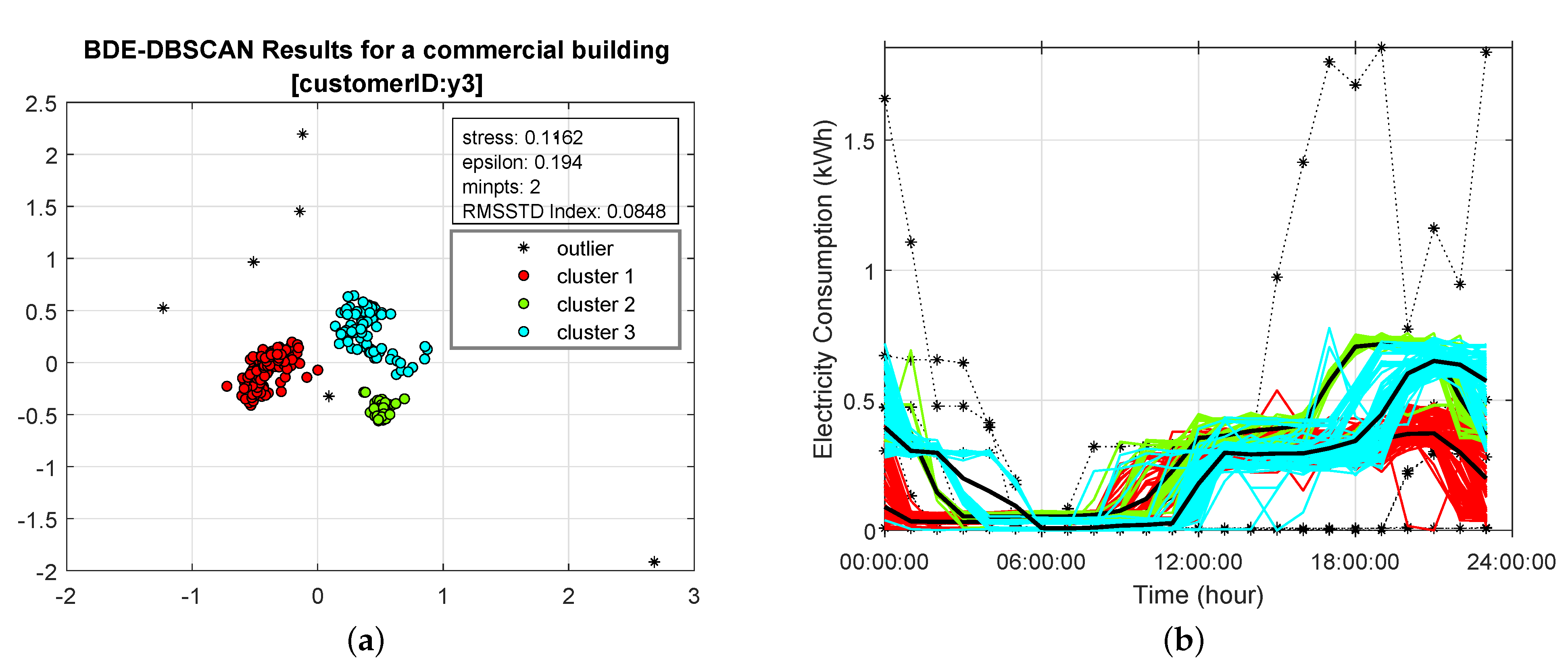
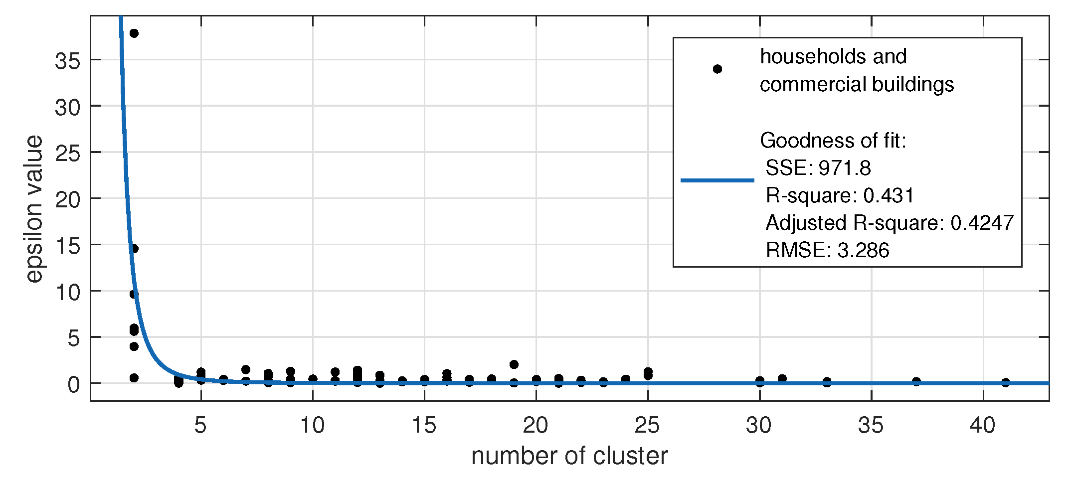
3.2. Density-Based Outlier Analysis of Daily Load Profiles

For evaluating the irregularity in daily load profiles, we implemented a different version of well-known density-based clustering method DBSCAN [23]. Some advantages of the DBSCAN algorithm compared to their counterparts are that it does not need to a predefined cluster number and includes outliers in the dataset. Moreover, the repeated consumption behaviors of customers form the main clusters, which makes the DBSCAN an ideal clustering technique fordetermining the daily consumption profiles that are not included in these clusters.
Therefore, the DBSCAN algorithm is well-suited for applications of extraction such as frequent patterns [23]. The algorithm requires three predefined parameters such as distance metric (Euclidean, Mahalanobis, Minkowski, etc.), the minimum number of object in a cluster ( m i n p t s ) , and the distance ( e p s i l o n ) values. The clustering results of the DBSCAN algorithm vary according to different m i n p t s and e p s i l o n values. An additional optimization process is required for the solution to this problem. In this study, a DBSCAN version based on binary differential evolution (binary differential evolution (BDE)) algorithm, proposed in [22] is preferred.
The algorithm BDE–DBSCAN uses binary coding for a ( m i n p t s ) population using a bit string. The second parameter ( e p s i l o n ) is determined in both an analytical and an iterative way in the optimization process. In the original study, the p u r i t y metric is determined for performance comparison on different data sets. The cost function ( p u r i t y ) needs to have both the input values and labels. Different from publicly available data sets, which possess both information, daily load profiles do not have predefined labels and this situation necessitates deciding on an alternative cost function at the stage of optimization. In this study, after extensive research, the root mean square standard deviation (RMSSTD) index is preferred as the cost function due to its simplicity and easy interpretation. Another modification in the proposed model is to use the RMSSTD index in an innovative way on both 2-D and N-dimension together to decrease the results of cost function. This adaptation is listed in lines 5 and 6 of the proposed Algorithm 1.
For the internal clustering validation metric, the root mean square standard deviation (RMSSTD) index is given in (4) [24].
RMSSTD = i x C i x c i 2 N i ( n i 1 )
where x represents a daily load profile ( x i = x i T · x i ) , and C i and c i represent the ith cluster and its center, respectively. N represents time resolution [24,48,96], as shown in Figure 1, and n i is the number of objects in C i .
The RMSSTD index evaluates the homogeneity of the resulting clusters in the optimization process [25]. Considering the ith customer’s resized data set after data cleansing, as illusturated in Figure 1, X [ K , N ] i = x ( 1 , N ) , x ( 2 , N ) , x ( 3 , N ) , , x ( K , N ) represents a data set in n-dimensional space, and K and N represent the number of available daily load profiles and time resolutions (24,48,96) of the related data set, respectively. After cluster label assignment, the data set X [ K , N ] is split into subsets based on its unique cluster number ( C = C 1 , C 2 , . . . , C i ) and then an average daily load profile, standard deviation, and sum of squares within cluster are calculated for each distinct subset. Lastly, a summation of mean squares for each subset is determined as in (4) and is obtained as a root-mean-squared (RMS) value. Additionally, in this study, the daily load profiles for which cluster label are assigned as (−1) are not included at the stage of RMSSTD index calculation, since the outliers are labeled as a default value of (−1) in the DBSCAN algorithm.

4. Forecasting Methods

4.1. Convolutional Neural Networks

The CNN algorithm is mostly preferred for image recognition tasks in deep learning applications. Unlike traditional approaches, the feature matrix is generated automatically from the convolution layer of CNN for classification and regression applications [26].
The convolution layers are designed based on the processing principle of the “convolution” operator, and the main purpose of this layer is to obtain useful features from input data by preserving correlation among data samples. The feature matrix is generated by shifting a filter over n-dimensional data, and then an additional activation function is applied for substituting entire negative values in the feature matrix by zero.
Since the CNN models are developed for image classification tasks, the input vector is represented on two dimensions such as image pixels and color information. A similar process can be implemented to 1-D sequential data, and the feature matrix can be obtained from a shifting process with a fixed period over time [27]. The main difference between multi-dimensional CNN models is the structure of data and how the convolution operator moves across data.

4.2. Long Short-Term Memory

The LSTM model was proposed by Hochreiter and Schmidhuber [28] to overcome the vanishing gradients. LSTM model has a similar structure to the RNN model, but each node of the hidden layer unit was replaced with a processing unit named “memory cell” and then improved with an additional unit “forget cell” by Gers et al. [29]. To guarantee the pass of the gradient through time without vanishing or exploding, each memory cell contains a recurrent node with a fixed weight. The basic structure of the LSTM cell consists of memory cells and gate units. The LSTM gate units are described as input gate i t , forget gate f t , and output gate o t . In this study, we preferred similar variable names as in [30] to formulate the LSTM model briefly.
Let x 1 , x 2 , x 3 , , x n represent a similar input sequence, where x n R k represents the k-dimensional input vector at the ( t + n ) th time step. The internal state of LSTM s t interacts with previous hidden state h t 1 and subsequent input sample x t to decide which internal state vector should be updated, maintained, or deleted based on previous output values and presents the input values. This structure of the LSTM builds temporal connections between memory cell states and maintains it throughout the whole process. Moreover, additional activation functions such as tanh and sigmoid are used in the LSTM memory cell. In the input node g t , both current input sample x t and recurrent weights from the previous hidden layer are passed through a tanh activation function. The equations of all nodes in a LSTM cell are given by (5) to (10),
g t = tanh w g , x x t + w g , h h t 1 + b g
f t = σ w f , x x t + w f , h h t 1 + b f
i t = σ w i , x x t + w i , h h t 1 + b i
o t = σ w o , x x t + w o , h h t 1 + b o
s t = g t i t + s t 1 f t
h t = tanh s t o t
where w · and b · represent weight matrices and biases, respectively; ⊙ represent element-wise multiplication; and σ symbolizes the sigmoid activation function. While the input gate is responsible for the update procedure of the memory unit, the output gate and the forget gate determine whether the current information will be maintained or erased in the unit. When the input gate takes the value zero, there is no change in the internal state of the LSTM structure and the memory cell preserves the present activation. This process continues along with intermediate time steps as long as both the input and the output gates are closed.

4.3. Bidirectional Long Short-Term Memory

The bidirectional RNN (BRNN), which was firstly introduced by Schuster and Paliwal in [31], utilizes both past and future information to determine the output values of an ordinary time series. Different from the LSTM network, in which merely previous information has an effect on output, this approach can be trained without the constraints of using a predefined input length. In the BRNN architecture, two different hidden layer nodes exist and these layers are connected with both input and output layers. While the recurrent unit of the first hidden layer has a connection with previous time steps through the forwarding direction, a similar connection is carried out in the opposite direction at the second hidden layer.
The BRNN can be trained with the same method used in a standard RNN. A standard feed-forward network unfolded through time can also be preferred due to the nonoccurrence of any interaction between hidden layers. The mathematical equations of BRNN are given by (11) to (13)
h t = σ w h , x x t + w h , h h t 1 + b h
e t = σ w e , x x t + w e , e e t + 1 + b e
y t = f ( x ) i × w y , h h t + w y , e e t + b y
where h t and e t represent the values of hidden layers in both the forward and backward directions of BRNN, respectively. Therefore, the LSTM and BRNN methods are suitable methods that can be used together. The LSTM method can compose a new unit that can be used in the hidden layer, while the BRNN method establishes a connection between these units. This approach is termed BLSTM and has been utilized in [32] for handwriting recognition and frame-wise phoneme classification.

5. Modeling Details

5.1. Data Descriptions

Due to the variety and volatility of energy consumption behaviors for residential and commercial consumers, short-term load forecasting is a complex prediction problem. Therefore, the performed strategy in the data collection of smart meters is randomly selecting customers to increase the robustness and reliability of the prediction model.
Therefore, a real data set that consists of one hundred different consumers’ information is used for the proof of concept. The data set contains in total 28,876 daily consumption profiles in Turkey of 56 households and 44 commercial buildings for 2018. After the data cleansing and outlier detection process, there are 22,505 load profiles that can be used for the proposed short-term load forecasting approach.
The collected variables from smart meters are customer ID, multiplier coefficient, time information, consumption values, and customers class, with dynamic data acquisition resolution according to customer preferences such as every 15 min, half hourly, and hourly.

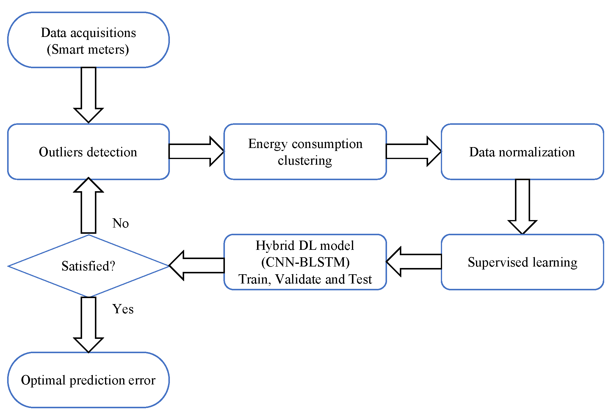
5.2. Advanced Preprocessing and Hybrid Dl Approach

Figure 2 shows the technical scheme of the proposed advanced preprocessing and hybrid deep learning approach, which includes collecting data from smart meters of a number of consumers, outliers detection, features clustering, normalization, supervised learning, and hybrid deep learning model. After careful decomposition, the data are prepared for supervised learning and split into different sub-datasets for training, validation, and testing. Then, the prediction model, which is hybrid deep learning CNN–BLSTM, learns and predicts load profiles of customers more accurately. If the prediction is not accurate enough, the model goes back to the outlier detection segment to remove further outliers; otherwise, the prediction is satisfying. In the following paragraphs, details about each segment are presented.
The cost function of the preprocessing model is based on the internal clustering validation metric (RMSSTD index). At the stage of parameter optimization of the DBSCAN algorithm, the main objective is to find the minimum RMSSTD index values. When this condition is satisfied, optimal parameters of the DBSCAN algorithm and the optimal training data set of the forecasting model are obtained. Therefore, the prediction accuracy is enhanced by optimal feature clustering and optimal training datasets. Otherwise, further feature clustering is applied to the preprocessing stage.
Considering the abovementioned electricity load data sets, household consumers lack consistent and cycled patterns due to the uncertainties of human behavior. Although commercial consumers tend to have more regular consumption patterns than residential consumers, there are uncertainties resulting from the workload. By preprocessing modelings proposed in this article, the forecasting model and results can be improved. Another obstacle can be listed as the deficiencies in smart measurement infrastructure services and the communication disconnection between smart meters and systems. This phenomenon has been also observed in our dataset. The ideal data acquisition scenario and the actual situation for residential building smart meters are shown in green and orange colors in Figure 3, respectively. It can be concluded that almost half of the smart meters do not have continuous data over one year period. Moreover, the blue area is the only suitable range for comparison of different customers’ consumption behavior.
In this study, non-metric MDS was implemented to N-dimensional data for dimension reduction. The m e t r i c s s t r e s s criterion is used to obtain 2-D subspace from N-dimensional data set. The m e t r i c s s t r e s s criterion is the normalized squared stress obtained from the sum of the fourth powers of the distance matrix [21,33]. A commercial building’s MDS representation and daily load profiles are shown in Figure 4a,b respectively. Each point in Figure 4a represents a daily profile of a commercial building over a year period.
After the dimension-reduction process, anomalous daily load profiles were detected using the BDE–DBSCAN algorithm and removed from the dataset. The RMSSTD index was chosen as the clustering validation metric, and the clustering process was repeated 30 times (epoch:30) for each individual. Due to the monotonicity issues of the RMSSTD index [34], two different strategies were implemented to overcome the issues; the first is using 2-D subspace for clustering and using a N dimension for calculating the RMSSTD validation index. The second strategy is keeping the minimum RMSSTD value, which consists of 100 iterations each, until the last iteration.
Implementation of the second strategy revealed some interesting hidden patterns in our data set. One of these patterns is shown in Figure 5. As can be seen, most residential and commercial buildings’ cluster number vary between 5 and 25, which is an acceptable cluster size considering individual consumption level [35]. Moreover, different percentages of anomalous days for all customers in the dataset are shown in Figure 6. This range also varied between 8–12% in general, and the white regions are not considered at this stage because these customers’ data sets consist of very small consumption values.
Another hypothesis can be obtained from clustering results represented in a chronological manner. A commercial building’s clustering calendar is shown in Figure 7. The days shown in gray and red on the calendar correspond to the situations where consumption values cannot be obtained and anomalous days that are represented as black stars in Figure 4b, respectively.
The anomalous days on the calendar are a good example of Hawkins’ definition of outlier “generated by a different mechanism” in [36]. Although these days cannot be included in any cluster, when examined carefully, it can be concluded that some of these days coincided with the religious holidays celebrated in Turkey. Other situations indicate three clusters with different colors in Figure 4b. It can be seen from Figure 7 that transition from one consumption behavior to another has generally an ordered structure. Although cluster changes are not observed in transition months (such as spring to summer or from autumn to winter) for this commercial building due to schedule or workload, an increase in the number of clusters is observed in almost half of the households in transition months (e.g., April to May or September to October).
The normalization process helps to limit the input values of all features within the 0 to 1 interval in order to avoid excessive feature values during the learning process as follows:
x i = x i x m i n x m a x x m i n
where x i is the original value of the input dataset, x i is the normalized value scaled to the range [ 0 , 1 ] , and x m a x and x m i n indicate the maximum value and minimum value of the features in x , respectively. Normalizing the dataset features eliminates the large deviation of instances, maps the data vector x to a small range vector x , and helps the learning algorithm to perform accurately.
The supervised learning form supports the learning in the training process by providing example pairs of the input to output prediction as follows:
y = H S L ( x )
where y is the normalized predicted energy load profile of the time series and H S L is the function of the supervised learning and the normalized output vector is defined as follows:
y = { y m , y m + 1 , , y m + n 1 }
where y i n is the mapped predicted load profile at a time i n and i n { m + 1 , m + 2 , . . . , m + n } and n is the number of future time prediction elements in the set y .
To evaluate the performance of the proposed prediction model properly, the testing set examines the trained and validated model independently. Therefore, we split the normalized supervised dataset into three sub-datasets (the training set 70%, validation set 20%, and the testing set 10%) in order to maintain the fairness of performance evaluation.
The learning in the prediction model segment is unlike the learning of traditional CNN or BLSTM models hybridized to improve the learning process. The first half of the prediction segment is the 1-D CNN, which is utilized to extract the input features and to encode them, and the second half is the BLSTM, which is used to analyze the extracted features from the 1-D CNN and to decode them for load prediction. The process of feature extraction in the 1-D CNN can sequentially capture the dynamics of the complex dataset and can determine complicated time series events.
The BLSTM model was formerly designed for text processing, which is difficult to analyse without using sequential inputs and outputs. The BLSTM consists of forward training and backward training to analyze and store information of sequential data. Therefore, training of the proposed hybrid DL model utilizes the 1-D CNN as a feature extraction of time series data and the BLSTM model for feature analysis. The training of the model is forward training in the feature extraction and the first part of the extracted feature analysis of BLSTM, where backward training is performed in the second stage of extracted feature analysis. The training process includes two layers of the 1-D CNN, with 64 filter size and 3 kernel size, to improve extracting the input features, and two layers of the BLSTM, with 50 hidden neurons and 25 hidden neurons, respectively, to analyze the extracted features and to predict the output. The activation function used in our model is rectified linear unit (ReLU), and the total number of training epochs is 100. The hyperparameters, including the number of hidden layers, the number of hidden neurons, activation function, loss function, and number of epochs, create an nondeterministic polynomial (NP) optimization problem for DL fine-tuning and complex stochastic process. In our modeling, the hyperparameters were selected based on a trial and error approach. The parameter settings of the proposed hybrid DL framework are presented in Table 1.
The development environment of our system is MATLAB, where preprocessing techniques were implemented, and Python 2.7, where the DL models were implemented with the Keras deep learning framework, and machine learning models were developed with the scikit-learn framework.

6. Forecasting Results and Discussion

The real data sets included load profiles of 56 households and 44 commercial buildings for the year 2018 with a one-hour resolution, and thus, contained a total of 28,876 daily consumption. After the outlier detection process, 22,505 daily consumption can be used to generate our proposed deep learning model.
The input of the prediction model is the historical energy consumption values of 100 customers in Turkey collected by the smart meters of the customers. The output of the proposed short-term load forecasting is precise future energy consumption prediction for one step ahead. The output of the forecasting results can deliver insights for utility company operators and building managers to modify their physical systems according to the predicted results.
To evaluate the forecasting performance results, we utilized 10% of the test dataset to examine the model after training and validation with 70% and 20% of the dataset, respectively. The conventional metrics used to evaluate the prediction models are utilized to evaluate the forecasting in our experiments. Traditional metrics such as the root-mean-squared error (RMSE); the coefficient of variation (CV) of RMSE, known as the normalized root-mean-squared error (NRMSE); MAE; and MAPE, are defined as follows (17) to (20):
RMSE = 1 m i = 1 m ( y i y ^ i ) 2
NRMSE = R M S E y ¯ × 100 %
MAE = 1 m i = 1 m | y i y ^ i |
MAPE = 1 m i = 1 m | y i y ^ i | y i × 100 %
where m represents the total number of data points in the time series, y ¯ represents the average of the actual values, y i is the actually measured time series in the original scale of the dataset, and y ^ i is the predicted output of the time series.
For the forecasting results section, several different evaluation criteria are utilized to evaluate the prediction performance models of residential and commercial buildings. The first criterion is directly bookmarking the average prediction metrics to conventional prediction models. Then, we compare the average prediction performance between residential buildings and commercial buildings within the clean data period (April– August). Third, we examine the preprocessing effects on our proposed prediction model for residential and commercial buildings with and without outliers. Lastly, we examine the time resolution effects on our proposed prediction model.

6.1. Comparison with Conventional Methods

Due to many promising results of deep learning-based load forecasting models [37], we should benchmark the results of our proposed model against conventional machine learning methods such as support vector regression (SVR) and decision tree (DT). Additionally, we should benchmark the results against conventional deep learning methods such as artificial neural networks (ANN) and conventional LSTM to explicate the out-performance of our proposed method. Nevertheless, we should compare our proposed model to a hybrid model CNN-LSTM.
The comparison methods preferred in the study are selected according to the rule of reproducible and interpretability. The parameter settings of SVR and DT models are determined according to the user guides of scikit-learn in [38,39], respectively. The rest of the comparison models parameter settings are presented in Table 2.
In the proposed work, we investigated several machine learning and deep learning models to find the optimal short-term load forecasting. First, we performed experiments over machine learning models that include SVR and DT. The performance of the SVR model is quite good in the average MAPE compared to other deep learning models. However, the DT model did not perform well for all the evaluation metrics. For instance, the average MAPE results of the machine learning models are 55.83% and 141.067 % for SVR and DT, respectively. However, these machine learning models did not perform well in the other evaluation metrics such as RMSE, NRMSE, and MAE. From Table 3, we can see that simple machine learning models lacks tackling the behavior of energy time-series data.
After extensive experiments on machine learning models and observing their performance with energy time series data, we performed experiments over several deep learning models including ANN, CNN, LSTM, BLSTM, and CNN–LSTM. From the experiments, the ANN model performed better than previous machine learning models such as SVR and DT in all evaluation metrics while the CNN, LSTM, BLSTM, CNN–LSTM models performed relatively close to each other. The proposed CNN–BLSTM model showed better performance in all evaluation metrics, with 0.108, 55.43, 0.058, and 36.75 RMSE, NRMSE, MAE, and MAPE, respectively. It attained the smallest error rate compared to all machine learning and deep learning models, as demonstrated in Table 3. The estimated load profile of a commercial buildings is illustrated in Figure 8.
To evaluate our model properly, we benchmarked our results against similar studies that used public data sets and are commonly applied for load forecasting in the literature for Smart Grid, Smart City [40] in Table 4. In this study, we implemented our proposed method to the same data set used in [41] and selected 69 customer’s consumption values between 1 June 2013 to 31 August 2013 time period. As can be seen in Table 4, our proposed model outperformed similar studies and we obtained an average MAPE value, 31.481, in the same testing interval.

6.2. Aggregated Forecasting with Clean Data

Considering different types of energy consumption applied in buildings, different time series behaviors were related to the type of buildings. In this experiment, we categorized the type of customers in buildings into residential and commercial. Additionally, we considered the clean data period from April to August 2018, when the data did not have many outliers and missing values. We performed the proposed model on these categories, as demonstrated in Table 5. The average forecasting errors for all residential buildings achieve 0.154, 71.73, 0.089, and 33.74 RMSE, NRMSE, MAE, and MAPE, respectively. The average errors for all commercial buildings achieve 0.135, 26.67, 0.084, and 27,37 RMSE, NRMSE, MAE, and MAPE, respectively.
From these error rates, we can conclude that aggregated forecasting for all commercial buildings obtains the smallest error rates in comparison to residential buildings. This is because most of the individual commercial buildings have relatively consistent behaviors and load profiles during this clean data period, while most of the individual residential buildings have the opposite, where their load profiles seem nonuniform and nonstationary.

6.3. Individual Customer Forecasting with Outliers Cancellation

In this section, the proposed model CNN–BLSTM is compared among every individual customer in the dataset for examining the preprocessing techniques that are mentioned in Section 5.2. In this experiment, we compared the forecasting results from the proposed model using original data with (w) outliers and data without (w/o) outliers. Indeed, we examined the effects of outliers in the data and after cleaning them and identified the percentage of improvement in individual customers, as shown in Table 6.
To know the impact of time series preprocessing on forecasting performance, we used the proposed model CNN–BLSTM for every individual customer in the dataset. We notice that the forecasting performance has been improved for almost every customer. In this experiment, we investigated the improvement percentage versus the number of customers that have been improved in each evaluation metrics. We conclude that the highest number of improved customers in evaluation metrics due to preprocessing techniques is in RMSE and MAPE in the improvement percentage range of 0–25%. The least number of improved customers is in the improvement percentage range of 75–100%. From these results, we can conclude that the preprocessing methods such as BDE–DBSCAN [22] have already improved the forecasting performance by using the proposed model by at least 25%.

6.4. Time Resolution Forecasting

In this experiment, we considered multiple scenarios of time resolution and time horizons by applying the proposed model after the preprocessing techniques (w/o) outliers. We defined multiple lookback time steps such as 1 h, 24 h, and 48 h for future energy consumption forecasting. The average forecasting performance of all customers for time resolution base is demonstrated in Table 7. All-time resolutions performed relatively similar to each other for all evaluation metrics; however, the one-hour resolution achieved the lowest error rates. We can conclude that the energy consumption behavior of hourly resolution provides a more accurate interpretation of the proposed model compared to daily and bi-daily consumption resolution.

7. Conclusions

Recently, short-term load forecasting of customer profiles has become a critical technique to build a robust and reliable system in the smart grid. This paper proposes advanced preprocessing tools and hybrid deep learning models that applied to one-hundred electricity consumers in 2018. The real data set contains the consumption information obtained with different time periods of 56 residential and 44 commercial buildings.
The purpose of the use of preprocessing techniques is to enhance the prediction accuracy by cleaning missing and corrupted data while collecting the dataset, which happens normally in most of data acquisition processes. Data aggregation, data cleansing, density-based clustering application for outlier analysis, and normalization were implemented at the preprocessing phase.
The effectiveness of the strategy proposed in this paper was confirmed by combining the preprocessing techniques with hybrid deep learning, which can ultimately build a robust and reliable prediction load forecasting. The proposed forecasting method is based on the hybrid version of CNN–BLSTM integrated with a density-based outlier analysis. The proposed model has a flexible structure that can generate feasible solutions on real data sets and can be rearranged depending on the application. Moreover, it is a reasonable option for the situations where it is difficult to obtain complete data acquisitions or that necessities using less features due to data privacy.
The forecasting model was evaluated according to different criteria. We conclude that the prediction performances of the proposed outperformed conventional prediction model. Considering the results obtained, the proposed method reduced MAPE values at different ranges for 72% of the dataset. Regarding the time complexity of training the proposed forecasting model, we found that it is inconsistent due to various customer load profiles and different factors such as dataset size, number of features, prediction model parameters, etc.
The analysis performed in the paper showed that the preprocessing tools coupled with the hybrid deep learning model CNN–BLSTM are powerful artificial intelligence tools for modeling robust load forecasting model and have the potential to be applied in different areas, such as smart grids, microgrids, and smart city, due to its outperformance, as illustrated.

Author Contributions

Conceptualization, F.Ü. and A.A.; methodology, F.Ü. and A.A.; software, F.Ü. and A.A.; validation, F.Ü. and A.A. and S.E.; formal analysis, F.Ü. and A.A. and S.E.; investigation, F.Ü.; resources, F.Ü. and A.A.; data curation, F.Ü., A.A. and S.E.; writing—original draft preparation, F.Ü., A.A.; writing—review and editing, F.Ü., A.A. and S.E.; visualization, F.Ü., A.A.; supervision, S.E.; project administration, S.E.; funding acquisition, F.Ü. and S.E. All authors have read and agreed to the published version of the manuscript.

Funding

This research was funded by the Firat University Scientific Research Projects Unit (FUBAP) grant number TEKF.20.25. This paper is also a part of the PhD. thesis of candidate F. Ünal in Firat University, Department of Energy Systems Engineering, Elazig, Turkey.

Acknowledgments

The authors would like to thank Mahmut Sami Sarac and Tolga Koc (Department of Automatic Meter Reading (AMR) System, Dicle Electricity Distribution Company) for providing helpful insights and supports for this project.

Conflicts of Interest

The authors declare no conflict of interest.

Nomenclature

X [ K , N ] i dataset of customer (i)
X a , b Euclidean distance between two daily load profile
X k , k distance (dissimilarity) matrix
X [ K , 2 ] two-dimensional (2-D) subspace projection
p a , b proximity between different daily load profiles
fmapping function of proximities
x i ith daily load profile
C i the ith cluster
c i the center of the ith cluster
Ntime resolution of the dataset [24,48,96]
B e s t S o l best solution of the BDE–DBSCAN algorithm for different parameters
P o p u l a t i o n [ i , i i ] generated population at the ith epoch and i i th iteration
x n k-dimensional input vector at the ( t + n ) th time step
g t input node of the LSTM model
s t internal state of the LSTM model
h t hidden state of the LSTM model
x t input sample at the tth time step
tanhactivation function of LSTM nodes
w · weight matrices of the LSTM cell
b · bias matrices of the LSTM cell
element-wise multiplication
σ sigmoid activation function of LSTM nodes
e t hidden state of BRNN
x i the normalized value scaled to the range [ 0 , 1 ]
x m a x the maximum value of the features in x
x m i n the minimum value of the features in x
y the normalized predicted energy time series
H S L the function of prediction model based on supervised learning
y i n the mapped predicted load at time i n
nthe number of future time prediction elements in the set y
mthe total number of data points in the time series
y i the actual measured time series in the original scale of the dataset
y ^ i the predicted output of the time series
y ¯ the average of the actual values of energy consumption

References

  1. Kong, W.; Dong, Z.Y.; Jia, Y.; Hill, D.J.; Xu, Y.; Zhang, Y. Short-Term Residential Load Forecasting Based on LSTM Recurrent Neural Network. IEEE Trans. Smart Grid 2019, 10, 841–851. [Google Scholar] [CrossRef]
  2. Tascikaraoglu, A.; Sanandaji, B.M. Short-term residential electric load forecasting: A compressive spatio-temporal approach. Energy Build. 2016, 111, 380–392. [Google Scholar] [CrossRef]
  3. Grolinger, K.; L’Heureux, A.; Capretz, M.A.; Seewald, L. Energy Forecasting for Event Venues: Big Data and Prediction Accuracy. Energy Build. 2016, 112, 222–233. [Google Scholar] [CrossRef] [Green Version]
  4. Almalaq, A.; Edwards, G. A Review of Deep Learning Methods Applied on Load Forecasting. In Proceedings of the 2017 16th IEEE International Conference on Machine Learning and Applications (ICMLA), Cancun, Mexico, 18–21 December 2017; pp. 511–516. [Google Scholar]
  5. Villalba, S.; Bel, C. Hybrid demand model for load estimation and short term load forecasting in distribution electric systems. IEEE Trans. Power Deliv. 2000, 15, 764–769. [Google Scholar] [CrossRef]
  6. Sun, X.; Luh, P.B.; Cheung, K.W.; Guan, W.; Michel, L.D.; Venkata, S.S.; Miller, M.T. An Efficient Approach to Short-Term Load Forecasting at the Distribution Level. IEEE Trans. Power Syst. 2016, 31, 2526–2537. [Google Scholar] [CrossRef]
  7. Ding, N.; Benoit, C.; Foggia, G.; Besanger, Y.; Wurtz, F. Neural Network-Based Model Design for Short-Term Load Forecast in Distribution Systems. IEEE Trans. Power Syst. 2016, 31, 72–81. [Google Scholar] [CrossRef]
  8. Cai, M.; Pipattanasomporn, M.; Rahman, S. Day-ahead building-level load forecasts using deep learning vs. traditional time-series techniques. Appl. Energy 2019, 236, 1078–1088. [Google Scholar] [CrossRef]
  9. Yong, Z.; Xiu, Y.; Chen, F.; Pengfei, C.; Binchao, C.; Taijie, L. Short-term building load forecasting based on similar day selection and LSTM network. In Proceedings of the 2018 2nd IEEE Conference on Energy Internet and Energy System Integration (EI2), Beijing, China, 20–22 October 2018; IEEE: Beijing, China, 2018; pp. 1–5. [Google Scholar] [CrossRef]
  10. Imani, M.; Ghassemian, H. Residential load forecasting using wavelet and collaborative representation transforms. Appl. Energy 2019, 253, 1–12. [Google Scholar] [CrossRef]
  11. Bedi, J.; Toshniwal, D. Empirical Mode Decomposition Based Deep Learning for Electricity Demand Forecasting. IEEE Access 2018, 6, 49144–49156. [Google Scholar] [CrossRef]
  12. Hossen, T.; Nair, A.S.; Chinnathambi, R.A.; Ranganathan, P. Residential Load Forecasting Using Deep Neural Networks (DNN). In Proceedings of the 2018 North American Power Symposium (NAPS), Fargo, ND, USA, 9–11 September 2018; IEEE: Fargo, ND, USA, 2019; pp. 1–5. [Google Scholar] [CrossRef]
  13. Enshaei, N.; Naderkhani, F. Application of Deep Learning for Fault Diagnostic in Induction Machine’s Bearings. In Proceedings of the 2019 IEEE International Conference on Prognostics and Health Management (ICPHM), San Francisco, CA, USA, 17–20 June 2019; IEEE: San Francisco, CA, USA, 2019; pp. 1–7. [Google Scholar] [CrossRef]
  14. Pathak, N.; Ba, A.; Ploennigs, J.; Roy, N. Forecasting Gas Usage for Big Buildings using Generalized Additive Models and Deep Learning. In Proceedings of the 2018 IEEE International Conference on Smart Computing Forecasting, Taormina, Italy, 18–20 June 2018; IEEE: Taormina, Italy, 2018; pp. 203–210. [Google Scholar] [CrossRef]
  15. Zheng, Z.; Yang, Y.; Niu, X.; Dai, H.N.; Zhou, Y. Wide and Deep Convolutional Neural Networks for Electricity-Theft Detection to Secure Smart Grids. IEEE Trans. Ind. Inform. 2018, 14, 1606–1615. [Google Scholar] [CrossRef]
  16. Qiu, D.; Liu, Z.; Zhou, Y.; Shi, J. Modified Bi-Directional LSTM Neural Networks for Rolling Bearing Fault Diagnosis. In Proceedings of the ICC 2019-2019 IEEE International Conference on Communications (ICC), Shanghai, China, 20–24 May 2019; IEEE: Shanghai, China, 2019; pp. 1–6. [Google Scholar] [CrossRef]
  17. Sehovac, L.; Nesen, C.; Grolinger, K. Forecasting Building Energy Consumption with Deep Learning: A Sequence to Sequence Approach. In Proceedings of the 2019 IEEE International Congress on Internet of Things (ICIOT), Milan, Italy, 8–13 July 2019; IEEE: Milan, Italy, 2019; pp. 108–116. [Google Scholar] [CrossRef] [Green Version]
  18. Su, H.; Zio, E.; Zhang, J.; Xu, M.; Li, X.; Zhang, Z. A hybrid hourly natural gas demand forecasting method based on the integration of wavelet transform and enhanced Deep-RNN model. Energy 2019, 178, 585–597. [Google Scholar] [CrossRef] [Green Version]
  19. Gao, Y.; Ruan, Y.; Fang, C.; Yin, S. Deep learning and transfer learning models of energy consumption forecasting for a building with poor information data. Energy Build. 2020, 223, 110156. [Google Scholar] [CrossRef]
  20. Ma, J.; Cheng, J.C.; Jiang, F.; Chen, W.; Wang, M.; Zhai, C. A bi-directional missing data imputation scheme based on LSTM and transfer learning for building energy data. Energy Build. 2020, 216, 109941. [Google Scholar] [CrossRef]
  21. Kruskal, J.B. Multidimensional scaling by optimizing goodness of fit to a nonmetric hypothesis. Psychometrika 1964. [Google Scholar] [CrossRef]
  22. Karami, A.; Johansson, R. Choosing DBSCAN Parameters Automatically using Differential Evolution. Int. J. Comput. Appl. 2014, 91, 1–11. [Google Scholar] [CrossRef]
  23. Ester, M.; Kriegel, H.P.; Sander, J.; Xu, X. A density-based algorithm for discovering clusters in large spatial databases with noise. KDD 1996, 96, 226–231. [Google Scholar]
  24. Sharma, S. Applied Multivariate Techniques; John Wiley and Sons, Inc.: Hoboken, NJ, USA, 1995. [Google Scholar]
  25. Gan, G.; Ma, C.; Wu, J. Data Clustering: Theory, Algorithms, and Applications (ASA-SIAM Series on Statistics and Applied Probability); Society for Industrial and Applied Mathematics: Philadelphia, PA, USA, 2007. [Google Scholar]
  26. Kim, J.; Moon, J.; Hwang, E.; Kang, P. Recurrent inception convolution neural network for multi short-term load forecasting. Energy Build. 2019, 194, 328–341. [Google Scholar] [CrossRef]
  27. Liao, G.; Gao, W.; Yang, G.; Guo, M. Hydroelectric Generating Unit Fault Diagnosis Using 1-D Convolutional Neural Network and Gated Recurrent Unit in Small Hydro. IEEE Sensors J. 2019, 19, 9352–9363. [Google Scholar] [CrossRef]
  28. Hochreiter, S.; Schmidhuber, J. Long Short-Term Memory. Neural Comput. 1997, 9, 1735–1780. [Google Scholar] [CrossRef]
  29. Gers, F.A.; Schmidhuber, J.; Cummins, F. Learning to Forget: Continual Prediction with LSTM. Neural Comput. 2000, 12, 2451–2471. [Google Scholar] [CrossRef]
  30. Lipton, Z.C.; Berkowitz, J.; Elkan, C. A critical review of recurrent neural networks for sequence learning. arXiv 2015, arXiv:1506.00019. [Google Scholar]
  31. Schuster, M.; Paliwal, K.K. Bidirectional Recurrent Neural Networks. IEEE Trans. Signal Process. 1997, 45, 2673–2681. [Google Scholar] [CrossRef] [Green Version]
  32. Graves, A.; Schmidhuber, J. Framewise phoneme classification with bidirectional LSTM and other neural network architectures. Neural Netw. 2005, 18, 602–610. [Google Scholar] [CrossRef] [PubMed]
  33. Borg, I.; Groenen, P.J.F. Modern Multidimensional Scaling Theory and Applications; Springer: New York, NY, USA, 2005. [Google Scholar] [CrossRef]
  34. Liu, Y.; Li, Z.; Xiong, H.; Gao, X.; Wu, J. Understanding of Internal Clustering Validation Measures. In Proceedings of the 2010 IEEE International Conference on Data Mining, Sydney, NSW, Australia, 3–17 December 2010; pp. 911–916. [Google Scholar]
  35. Jin, L.; Lee, D.; Sim, A.; Borgeson, S.; Wu, K.; Spurlock, C.A.; Todd, A. Comparison of Clustering Techniques for Residential Energy Behavior Using Smart Meter Data. In AAAI Workshop—Technical Report; Association for the Advancement of Artificial Intelligence (AAAI): San Francisco, CA, USA, 2017. [Google Scholar]
  36. Hawkins, D.M. Identification of Outliers; Springer: Berlin/Heidelberg, Germany, 1980; Volume 11. [Google Scholar]
  37. Yildiz, B.; Bilbao, J.; Dore, J.; Sproul, A. Recent advances in the analysis of residential electricity consumption and applications of smart meter data. Appl. Energy 2017, 208, 402–427. [Google Scholar] [CrossRef]
  38. sklearn.svm.SVR—scikit-learn 0.24.1 Documentation. scikit-Learn. 2018. Available online: https://scikit-learn.org/stable/modules/generated/sklearn.svm.SVR.html/sklearn.svm.SVR (accessed on 13 March 2021).
  39. sklearn.tree.DecisionTreeRegressor—scikit-learn 0.24.1 Documentation. scikit-learn, 2018. Available online: https://scikit-learn.org/stable/modules/generated/sklearn.tree.DecisionTreeRegressor.html/sklearn.tree.DecisionTreeRegressor (accessed on 13 March 2021).
  40. Smart Grid, Smart City. Australian Govern, 2014. Available online: https://webarchive.nla.gov.au/awa/20160615043539; http://www.industry.gov.au/Energy/Programmes/SmartGridSmartCity/Pages/default.aspx (accessed on 6 October 2020).
  41. Alhussein, M.; Aurangzeb, K.; Haider, S.I. Hybrid CNN-LSTM Model for Short-Term Individual Household Load Forecasting. IEEE Access 2020, 8, 180544–180557. [Google Scholar] [CrossRef]
Figure 1. Modelling framework of the proposed outlier detection.
Applsci 11 02742 g001
Figure 2. Proposed prediction model scheme.
Applsci 11 02742 g002
Figure 3. The optimal range for comparison of different household’s daily electricity consumption.
Applsci 11 02742 g003
Figure 4. Non-classical multidimensional scaling representation (a) and daily consumption profiles (b) of a commercial building (customer ID: y3 and BDE–DBSCAN clustering result).
Applsci 11 02742 g004
Figure 5. The relation between epsilon values versus number of clusters in dataset.
Applsci 11 02742 g005
Figure 6. Percentage of different categories in dataset.
Applsci 11 02742 g006
Figure 7. Clustering calendar of a commercial building in 2018 (customer ID: y3).
Applsci 11 02742 g007
Figure 8. Estimated load profile of a commercial building (customer ID: y3).
Applsci 11 02742 g008
Table 1. Parameter settings of the proposed model.
ParameterSetting
CNN-1D filter size64
CNN-1D Kernel size3
BLSTM 1s hidden layer50 hidden neurons
BLSTM 2nd hidden layer25 hidden neurons
OptimizerReLU
Loss functionMean square error (mean square error (MSE))
Learning rate0.001
Batch size120
Epoch100
Table 2. Parameter settings of comparison models.
Design Parameters of the Comparison Methods *
MethodN. of Hidden NeuronActivation FunctionBatch SizeFilter SizePool SizeOptimizer
ANN500sigmoid500--SGD **
CNN-ReLU20064-ADAM
LSTM200sigmoid200--SGD
BLSTM50-200--ADAM
CNN-LSTM50/25ReLU200641ADAM
* The epoch and loss function are set to 100 and MSE, respectively, for all models. ** stochastic gradient descent (stochastic gradient descent (SGD)).
Table 3. Performance of different machine learning and deep learning models.
MethodRMSE (kW)NRMSE (%)MAE (kW)MAPE (%)
SVR0.194206.1070.12555.826
DT0.242102.4700.141141.067
ANN0.15482.5290.10954.719
CNN0.14361.1900.08857.675
LSTM0.12967.5800.07745.084
BLSTM0.13154.8250.07846.452
CNN-LSTM0.14863.6240.08846.755
Proposed0.10855.4320.05836.748
Table 4. Benchmarking of different studies using mean absolute percentage error (MAPE) criterion.
ReferencePublicDatasetForecastingTestingMAPE
Dataset NameSize *MethodInterval(%)
Kong et al. [1]Smart Grid69LSTM23-Aug-2013 to44.060
Smart City 31-Aug-2013
Alhussein et al. [41]Smart Grid69CNN-LSTM23-Aug-2013 to40.380
Smart City 31-Aug-2013
ProposedSmart Grid69CNN-BLSTM23-Aug-2013 to31.481
Smart City 31-Aug-2013
* The dataset size is determined by considering the subsets selected for forecasting experiments (number of customers).
Table 5. Performance of aggregated forecasting for different buildings types in the period April to August 2018.
BuildingRMSENRMSEMAEMAPE
Type(kW)(%)(kW)(%)
Residential0.15471.7280.08933.736
Commercial0.13526.6720.08427.374
Table 6. Improvement (%) distribution of the testing results.
ImprovementResidential and Commercial Building *
PercentageRMSENRMSEMAEMAPE
(kW)(%)(kW)(%)
(<0)%18261624
(0–25)%35252935
(25–50)%24252616
(50–75)%671212
(75–100)%5551
* Total available customer number for improvement comparison is 88 due to some issues mentioned in Section 5.2.
Table 7. Forecasting results of proposed method with different time steps.
MethodTimeRMSENRMSEMAEMAPE
Steps(kW)(%)(kW)(%)
CNN-BLSTM1 h0.10855.4320.05836.748
-without(w/o)24 h0.10856.4780.05936.911
outliers48 h0.10856.1440.05938.008
Publisher’s Note: MDPI stays neutral with regard to jurisdictional claims in published maps and institutional affiliations.

