Damage Evolution Analysis in a “Spaghetti” Bridge Model Using the Acoustic Emission Technique

Abstract

This paper applies the Acoustic Emission (AE) Technique to analyze the damage process in a one-meter span bridge model that was built from spaghetti sticks during a loading test. The AE signals are analyzed in terms of four coefficients that are evaluated as predictors of structure failure, with frequency variation appearing to be the strongest indicator of instability. The AE data are also compared to theoretical predictions that are given by the Bundle Model, confirming that underlying general patterns in damage processes are highly influenced by the geometric distribution of the structure and the loading pattern that is applied to it.

1. Introduction

The damage process in structures or materials undergoing unstable collapse is a widely studied topic, because it occurs in many different situations, including catastrophic events with heavy human and economic tolls. This process is particularly important in the case of heterogeneous materials, such as rocks, concrete ceramics, and other composites, either natural or artificial. According to Krajcinovic [1], the main phenomena characterizing damage processes in these materials are: (i) significant size-effects in the strength and failure strain, (ii) transitions from uniform damage distribution to a clear discontinuity process, known as cracks localization, and (iii) the associative effect among clusters of micro-cracks, which can either intensify or inhibit damage propagation throughout the structure during the process.

Continuous regularization functions can represent model parameters describing damage evolution, which filter a series of discontinuities distributed throughout space and time, thus providing valuable information regarding the ongoing damage process, indicating how and when a significant loss of material resistance can occur. In its turn, collapse study by means of an apparently simple theoretical models allows for one to avoid the specifics of each structure and to perceive tendencies that are common to several systems, regardless of building materials, boundary conditions, and problem scale. Some such models are discussed in [2]. Being aided by these models, one can describe laws that apply to processes ranging from the rupture of biological materials of microscopic dimensions [3], to seismological events throughout hundreds of kilometers [4,5].

Besides pure Mechanics, similar patterns can be found in other realms of Physics, most notably the method of renormalization groups that was proposed by Wilson [6], which allows for coping with instability problems, such as the disruption of solids and phase changes. These ideas also apply to other instability problems, like those found in time series of economic indexes [7], the degradation of social systems [8], and the collapse of ancient civilizations [9]. In all of these cases, studying the evolution of local instabilities throughout space and time is a fundamental step in predicting global instability.

In mechanics, a suitable way to register local instabilities is the Acoustic Emission (AE) technique. Whether caused by a chemical reaction (metal corrosion), the spasmodic growth of vegetal, or an impact from an external source, among many other examples, when a local instability occurs, it is said to generate an event in a specific structure location, called source. This event causes the propagation of mechanical waves that are perceived by sensors on the structure’s surface. By placing various sensors on suitable locations of the structure, space and time distribution of these events can be determined, and the parameters that are calculated from such measurements are a sensitive means for tracking changes within the studied structure.

Here, we apply the AE technique to track a small-scale bridge that is built from spaghetti sticks. As the bridge is subjected to increasing load, two sensors acquire the AE signals. Measurement results are compared to theoretical predictions according to the Bundle Model [10], which is widely used in this field [11]. This comparison’s primary goal is to highlight the possibility of an underlying universal pattern for structures in collapse, which is often masked by specifics in geometry and boundary conditions imposed on each structure. The use of a spaghetti bridge as the basic structure for the study facilitates the execution of typical material tests —e.g., three-point bending and uniaxial compression in a cylinder— on an easy to build, inexpensive specimen. Riazi et al. [12] have also explored this possibility, applying artificial intelligence methods to determine the collapse load on a similar bridge.

2. Theoretical Foundations

This work is based upon two basic tools: the Acoustic Emission technique and the Bundle Model. The basic principles of each tool will be presented in this section.

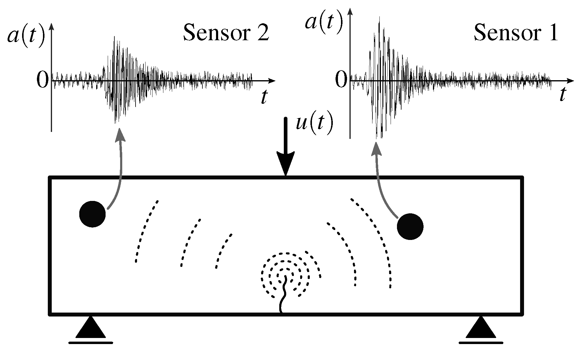
2.1. Acoustic Emission Technique

When a mechanical system is excited by an external source or undergoes changes in its internal structure, it presents local instabilities (events) that propagate as mechanical waves. These Acoustic Emission (AE) signals are usually accelerations with frequencies ranging from ${10}^4$ to ${10}^7$ $\mathrm{Hz}$ [13]. These signals are detected by accelerometers that are mounted on the structure’s surface, as depicted in Figure 1, where the excitation is usually a force or prescribed displacement in time.

Figure 2 illustrates a typical AE signal. Several parameters can be extracted from these signals [13], but the ones of interest here are: maximum Amplitude ($A_p$), signal threshold ($A_{th}$), initial time ($t_i$), and final time ($t_f$), where both times are functions of the fixed threshold level. The Rise Time ($R_T$) is defined as $R_T=t_p-t_i$, i.e., the difference between the instant of maximum amplitude ($t_p$) and the moment $t_i$ when amplitude rise from threshold levels was first detected. From these data, the Rise Angle ($R_A$) is given by $R_A=R_T/A_p$. Finally, the area under the signal is also of interest, because it bears a direct relation with the acoustic energy emitted during the event, as explained in detail in [14].

Besides having their own meaning regarding both spatial and temporal distributions of the events in AE tests, these parameters can also be combined, generating reliable indicators regarding the possibility of system collapse. Such indicators are:

(a)

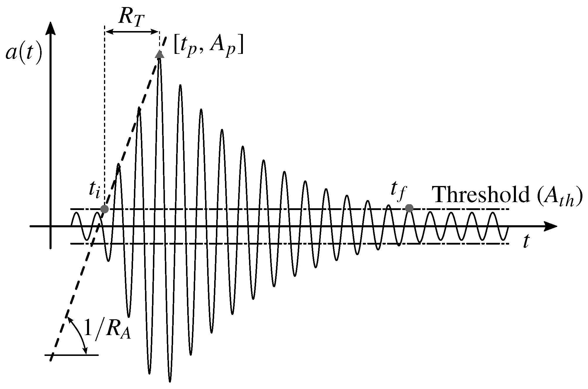
Relation between the number of events N and the signal amplitude A: this relation has been long used in seismological applications, as illustrated by the classic Gutenberg & Ritcher law [4], which is of universal nature and it does not depend on the scale of the distribution [11,15,16]:

$$N(\ge A)\propto A^{-b},$$

(1)

where N is the cumulative number of signals and A is the signal amplitude. The physical meaning is discussed in [17,18,19]. It is hypothetically related, according to the expression $\mathcal{D}=2b$, to the fractal dimension $\mathcal{D}$ of the material domain from which the signals that are generated by cracks are emitted. When the damage process begins within a structure, signals are emitted from a micro-cracks roughly evenly distributed in the material volume, i.e., $\mathcal{D}=3$ and $b=1.5$. Thus, according to Equation (1), most events produce small-amplitude signals. As damage advances, localization effects take place, and the signals are preferentially emitted from micro-cracks that distribute on preferential surfaces, which results in macro-crack nucleation. Therefore, in this last phase, the values for $\mathcal{D}$ and b become 2 and 1, respectively, and the application of Equation (1) yields an increase in the number of large-amplitude events. Thus, the evaluation of b and how it changes with time allows for one to keep track of damage processes.

The procedure for computing b is schematically described in Figure 3a. The amplitudes due to each signals are collected and organized in a histogram. Subsequently, a bi-log diagram is built to illustrate the cumulative number N of signals with amplitude $\ge A$. Finally, b is the angular coefficient of the fitting line. For a more detailed discussion about this computing procedure, see [20].

(b)

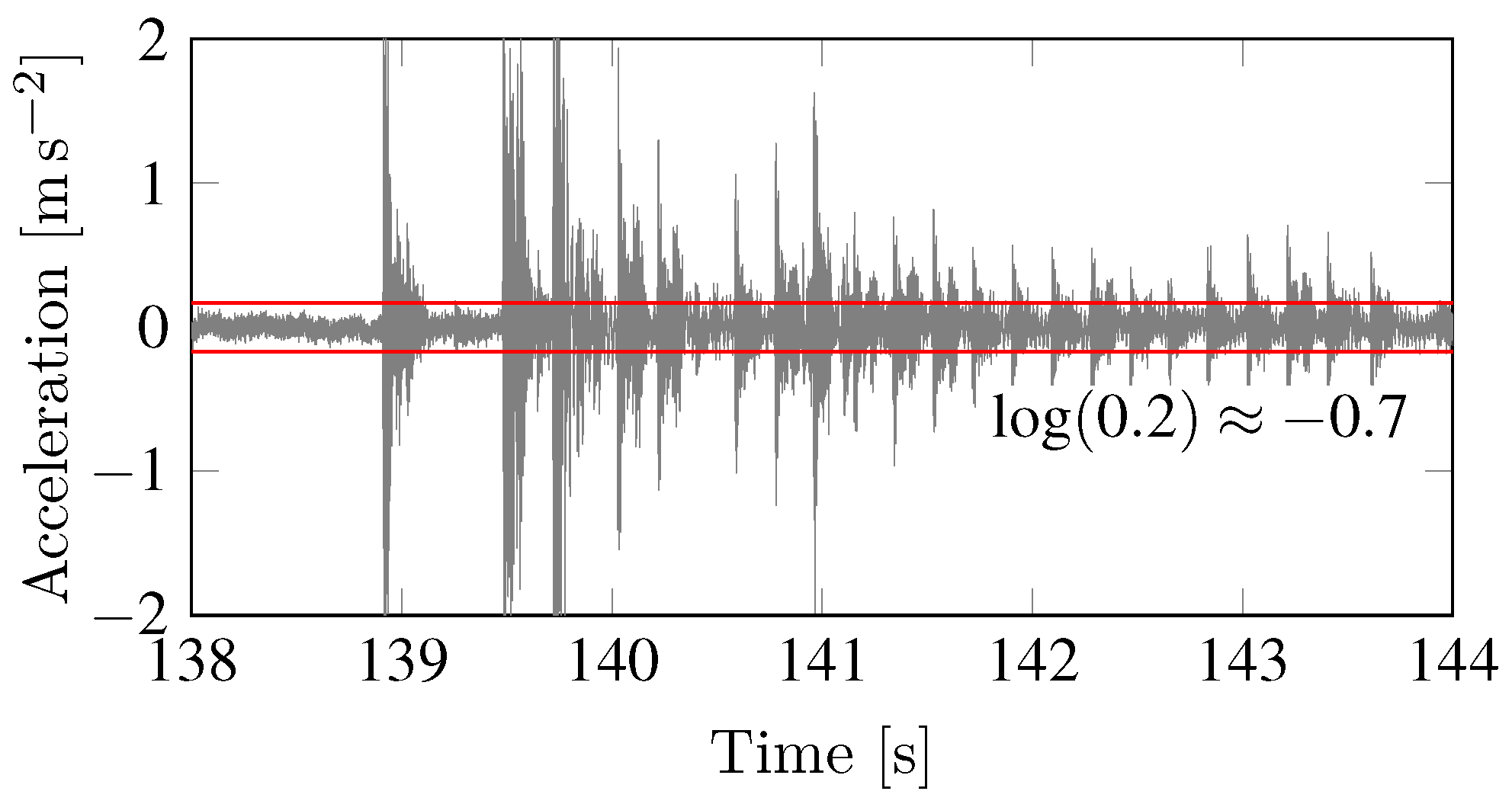
Relation between N and the signal energy emission $E_s$: the energy that is carried in the signal is also related to N in a form similar to that of the amplitude A, using $ϵ$ a fitting coefficient analogous to b:

$$N(\ge E_s)\propto {E_s}^{-ϵ}.$$

(2)

The calculation of $ϵ$ is analogous to the one described for b in case (a). It is also described in Figure 3a. Because the emitted AE signal energy is proportional to the squared maximum amplitude ($E_s\propto A^2$), it is apparent that the expected interval for b [1.0, 1.5] translates to [0.5, 0.75] for $ϵ$, as discussed in [2] and shown by numerical simulation in [21]. One can also compute the energy emission from the area under the signal envelope, as also indicated in Figure 3b. This approach, referred to here as the RILEM method, was proposed in [13,22]. Finally, it is also possible to calculate energy emission from the Root Mean Square of the signal.

(c)

Relation between N and the characteristic signal frequency $f_s$: this parameter was introduced by the same research team involved in this work as a reliable indicator for avalanches during a damage process [23]. This newly introduced coefficient c is also obtained by analogous means to those that are given for Equations (1) and (2), but focusing on the frequency distribution of the AE signals, i.e.,:

$$N(\ge f_s)\propto {f_s}^{-c}$$

(3)

where N is the cumulative number of signals with frequencies greater or equal to $f_s$. The value of c can be similarly calculated to that used for b, as indicated in Figure 3c: it is the slope line of the signals distribution during the damage process as a function of the frequency that characterizes the signals. As in the case of the b-value for amplitudes, the c-value indicates changes in the damage process and the imminence of collapse by keeping track of the acquired AE signals’ frequencies. For instance, if the number of events with lower characteristic frequencies increases as compared to the higher ones, a change in the damage process has occurred.

Still, regarding Figure 3c, note that there are two ways to calculate the characteristic frequency $f_s$ of the AE signal. The first is taking the ratio between the number of cycles np and the signal time interval ($t_f-t_i$), as proposed by the RILEM [22] and referred to here as RILEM frequency. An alternative definition is by determining the spectral distribution of the AE signal and taking the frequency with the highest peak, i.e., the FFT method.

(d)

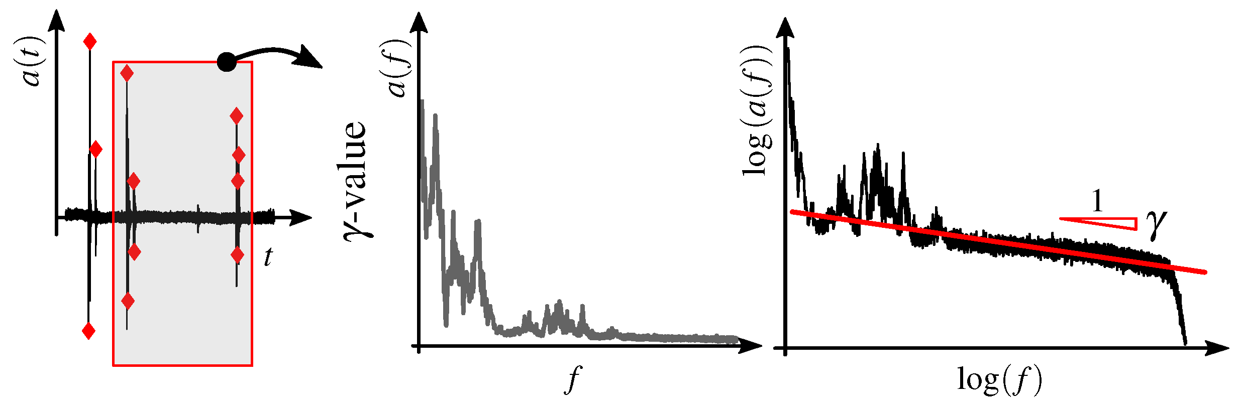
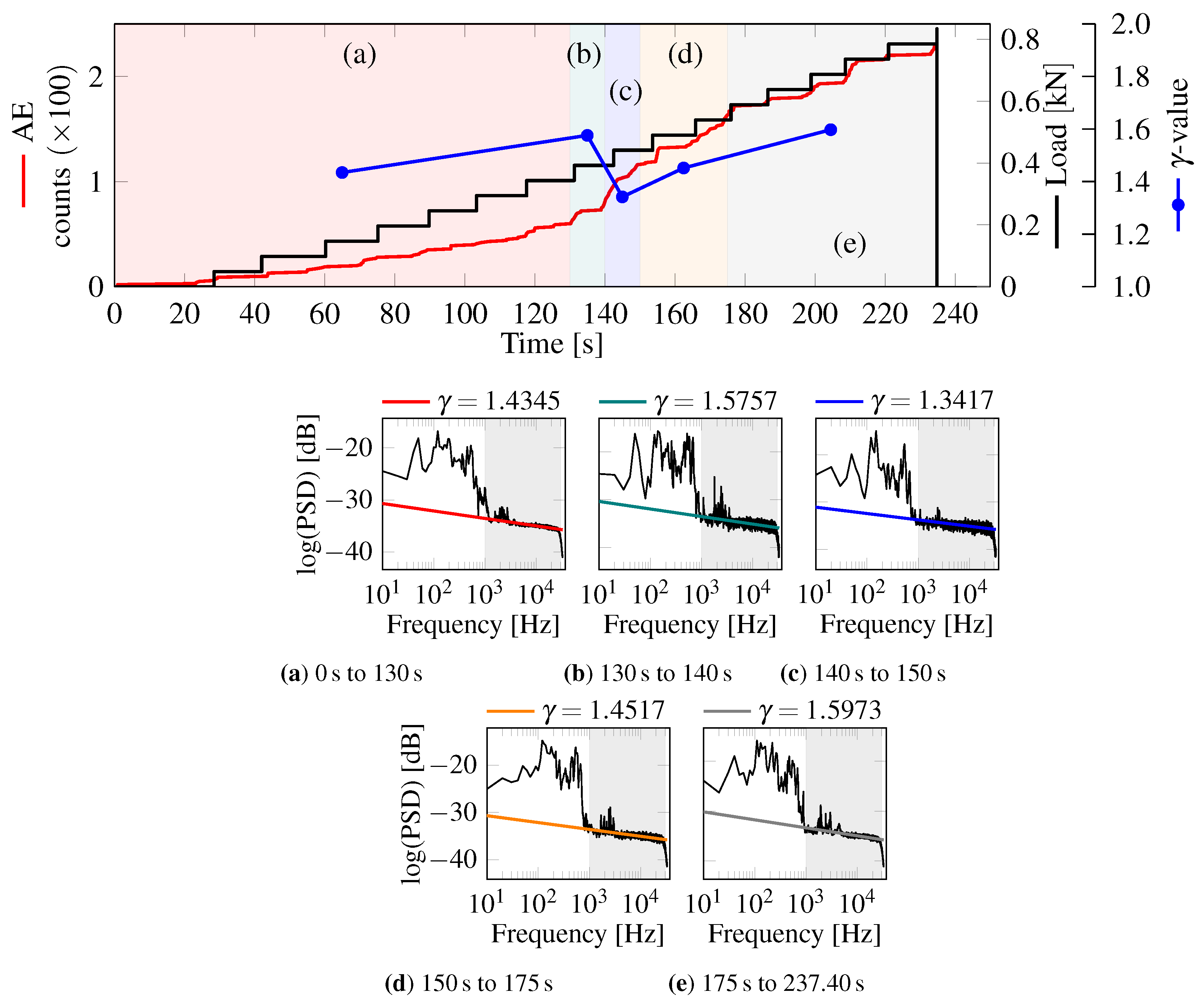
Frequency fluctuations during the damage process: a well-known measure of energy fluctuations in AE signals relies on their dependence on signal frequency, as described by the spectral density function (SDF), as mentioned by [24]. The first observations regarding this dependence are reported by [25], who coined the term $1/f$-noise or Flicker Noise when studying the noise effects in electronic circuits. According to [26], the dependence of noise energy distribution with respect to frequency is given by:

$$E\left(f\right)=a1/f^{\gamma },$$

(4)

where $E\left(f\right)$ is the energy emission, f is the signal frequency, while $\gamma$ and a are the scalar fitting coefficients. Taking the logarithm of both sides in Equation (4), the best fitting line leads to a linear law, where gamma is the angular coefficient. Its calculation is schematically described in Figure 4.

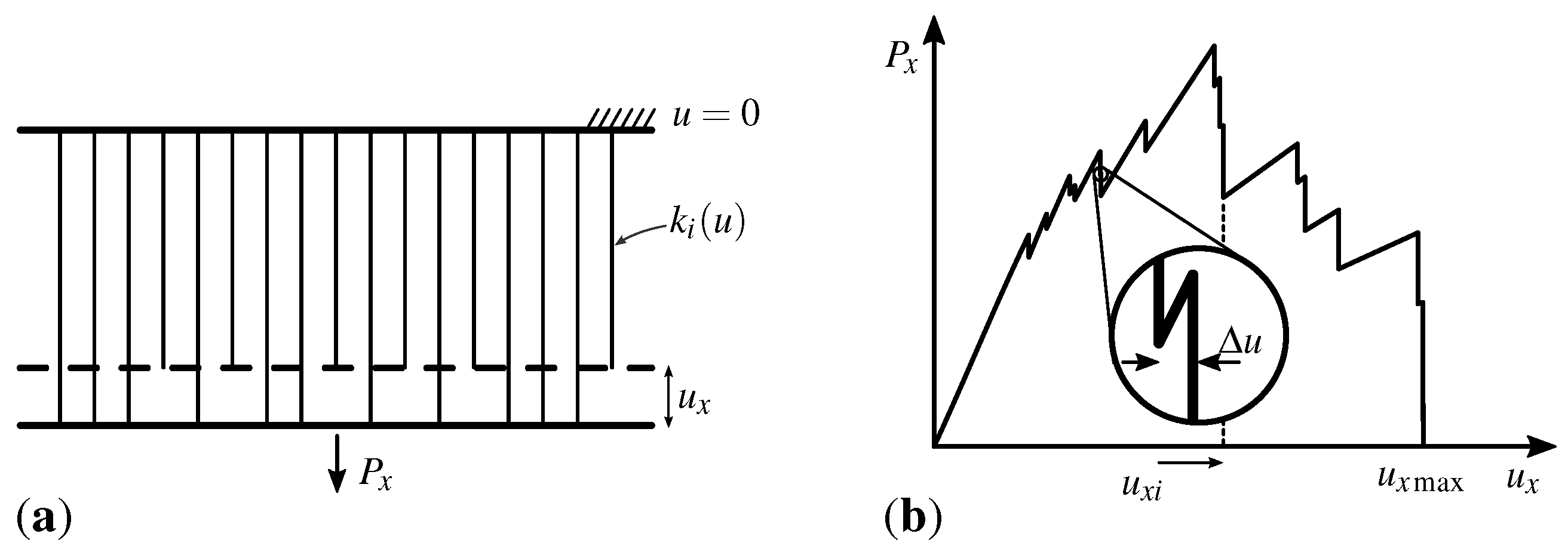
This type of fluctuation is widely observed in many different scientific fields, such as geology [27], finances [28], bioengineering [29], and even music [30,31], as observed in [32] and many other works. Moreover, the distributions described in Equation (4) is also observed to hold for frequencies ranging from fractions of hertz (in seismology) to gigahertz (microelectronics), which clearly illustrates the fractal character of this distribution and the phenomena to which it applies [32]. In the specific case of Acoustic Emission applications, the study of damage in historic buildings by [33] is an interesting example, where the exponent changes in the imminence of (either local or global) instabilities that are associated with structural collapse.

Notice that the global parameters (b, $ϵ$, c, or $\gamma$ values) do not depend on the counts’ number N in itself, but on the statistic distribution of magnitude and frequency for each count. For instance, b and $ϵ$ tend to higher values if most of the counts are of low magnitude. As the proportion of high-amplitude counts increase, there is a decrease of these parameters. Similarly, decreases in c or $\gamma$ coefficients indicate that events of all scales participate in the signal, thus causing a wide frequency range to be excited. This agrees with Wilson [6]: all of the scales participate in the system response when the critical regime is near.

2.2. Bundle Model

Peirce (1926) [34] initially proposed the Bundle model to investigate the strength of cotton cloth, whereas Daniels [10] established its statistical foundations in 1945. Many other works also have used this model in the study of fracture of fiber-reinforced composite, with [35,36] as recent examples. The use of the Bundle Model also appears in the study of snow avalanches and landslides, as in Lehmann and Or (2012) [37] and Cohen et al. (2011) [38].

To the authors’ knowledge, the most relevant application of this method is the one by Sornette (1989) [39], which uses it as a tool to represent the behavior of solids undergoing damage processes. A comprehensive discussion of the Bundle Model and its applications is presented in the book by Hansen et al. (2015) [11]. Its simplest version is the Equal Load Shared Bundle Model (ELS Bundle Model), which comprises a set of parallel fibers (Figure 5a) with both ends fixed to a rigid frame. Each fiber is assumed to have elastic behavior until reaching its respective failure strength, which is given by a known statistical distribution. Figure 5b presents the typical load vs prescribed displacement for this setup. In the classical paper by [15], it is shown that, when a continuously increasing displacement is prescribed to the set of fibers (i.e., the set is continuously stretched by infinitesimal increments), the distribution of number of broken bars is given by an exponential function with a universal exponent of $-2.5$, regardless of the specific distribution of failure strength in the fibers.

The ELS Bundle Model also predicts two forms of distributions that deviate from the aforementioned universal one, as shown in Figure 6 [11]. The first deviation takes place when the prescribed displacement is continuously increased only to a value $u_{xi}<u_{max}$, i.e., the loading process is interrupted before the critical displacement for complete failure is reached. In this case, since the available data do not reflect the entire failure process, the model’s predictions deviate from the universal distribution, as shown in Figure 6a. The second form occurs when the prescribed displacement occurs in discrete steps. Now, each step is large enough to cause failure of several fibers at once, causing the prediction curve to draw away from the ideal straight line at the top left of the graph, as shown in Figure 6b.

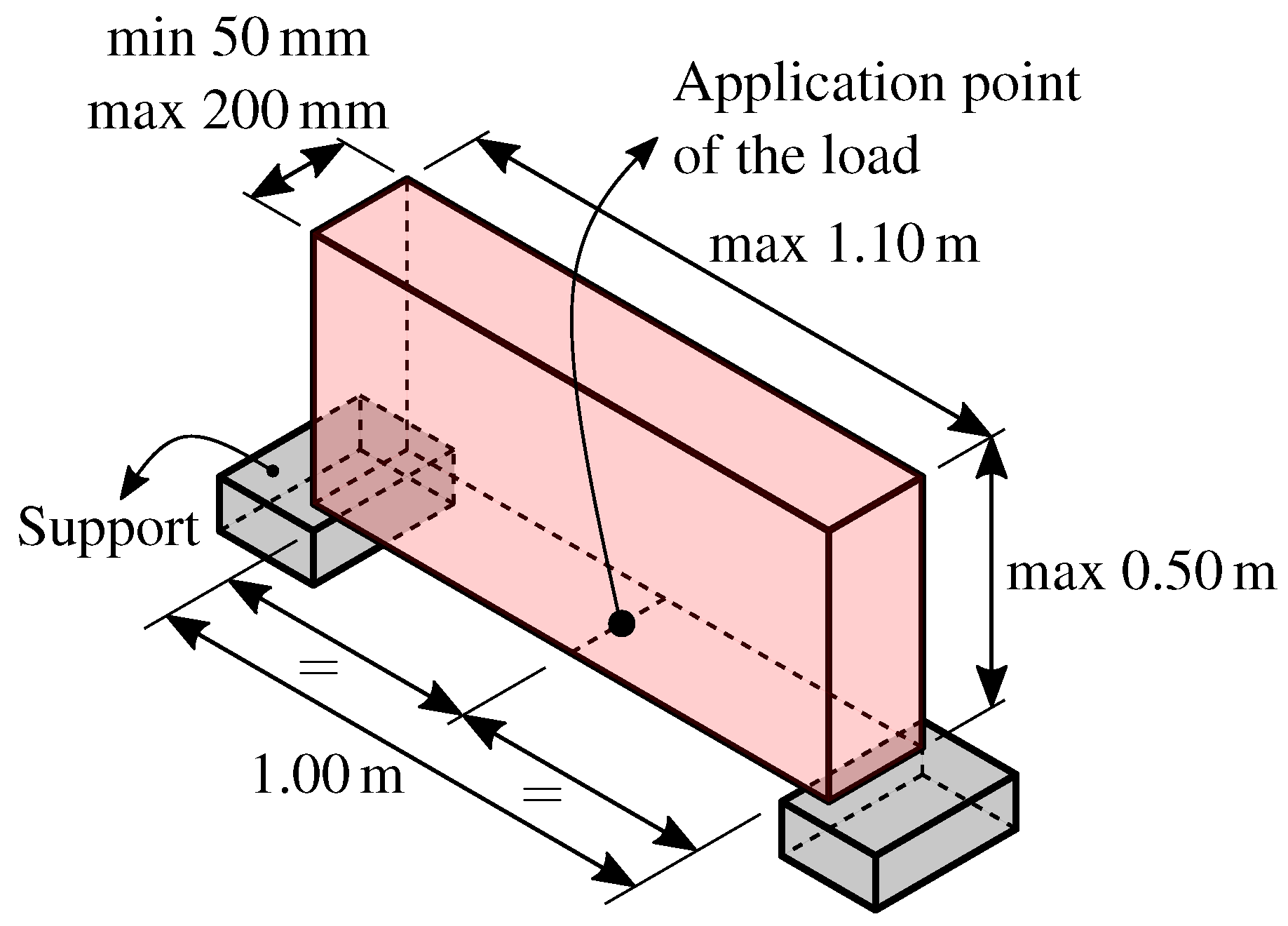
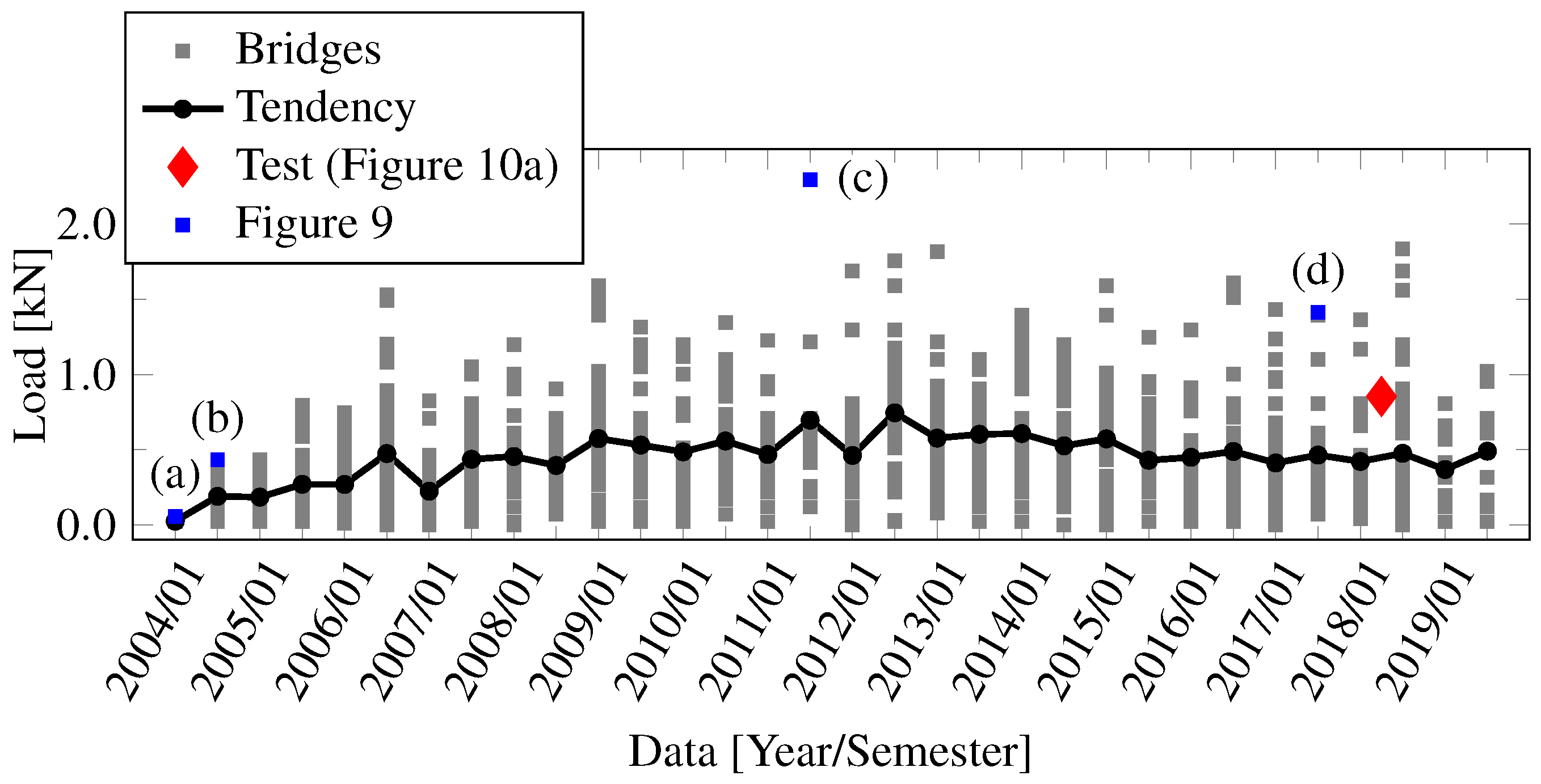
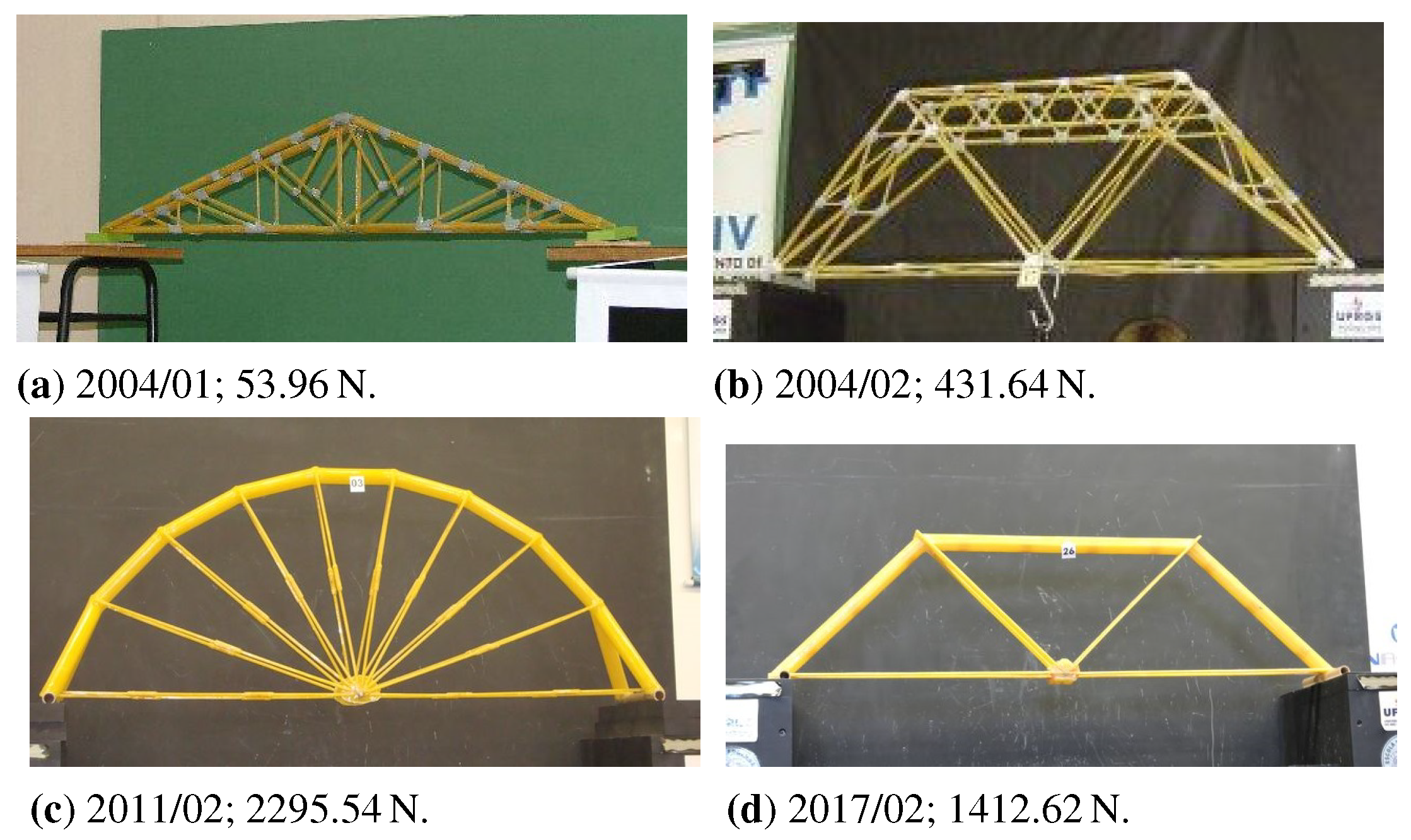
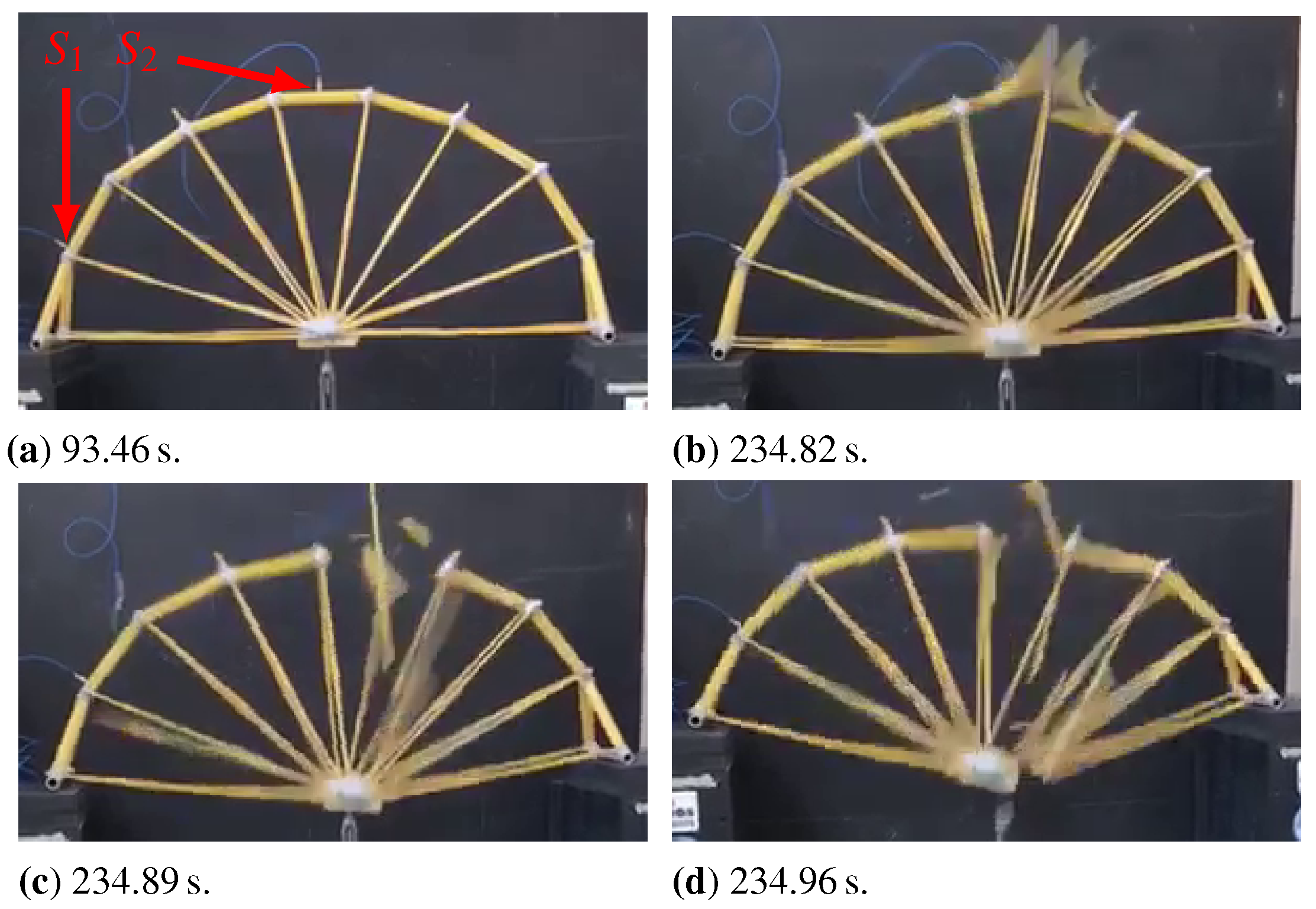
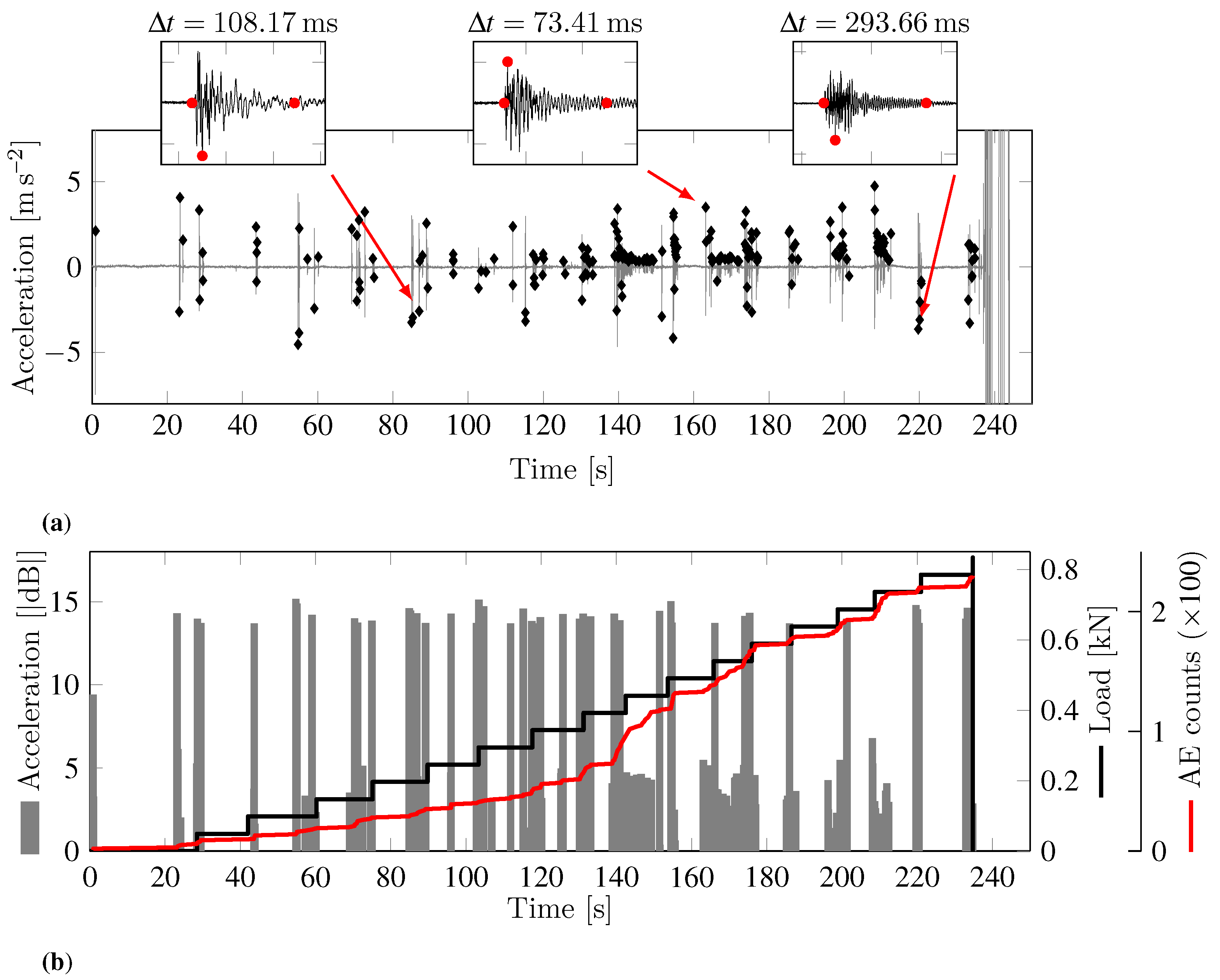
3. Application: The Bridge Model Analysis

The technique was applied to a small-scale bridge model made from spaghetti sticks, built by undergraduate students taking part in a contest, in order to illustrate the effectiveness of the global parameters’ evolution obtained from an AE analysis method as predictors of structure collapse. The idea of spaghetti bridge contests was initially proposed in the Okanagan College in 1980 [40], to motivate the students in the basic concepts of building actual structures. Nowadays, similar initiatives occur in several educational institutions around the world. The structure that was analyzed here was built for the contest at the Engineering School of Federal University of Rio Grande do Sul (UFRGS), which occurs twice a year since 2004. Participation in the context is mandatory for Civil Engineering students, but it is also open to students from all other Engineering programs. This bridge model complies with all guidelines for the contest (geometric restrictions, mass limits, load application, etc.), described in detail in [41,42], and its main geometric parameters appear in Figure 7.

The collapse loads for all bridges evaluated in the contest are informed in Figure 8, with four winning designs being highlighted in the same figure and depicted in Figure 9. It is noticed that the average collapse load increases for the first six years, tending to an approximately constant value after that. This is due to the increased tendency of most contestants to adopt the topology that is depicted in Figure 9c, which is theoretically optimal for stiffness [43].

Figure 10 depicts the spaghetti bridge used in the AE test, undergoing its load test during the contest, and its corresponding collapse load is also highlighted (in red) in Figure 8. This bridge was $1.08$ $\mathrm{m}$ long, $0.15$ $\mathrm{m}$ wide and $0.45$ $\mathrm{m}$ high, with $1.401$ $\mathrm{k}\mathrm{g}$ of mass. Load was increasingly applied manually to its center line, with increments in 10 $\mathrm{s}$ intervals until collapse occurred at $t=235\mathrm{s}$, with $784.8$ $\mathrm{N}$. Two accelerometers [44] were installed on the spots that are marked as $S_1$ and $S_2$ in Figure 10a, for acquiring the AE signals. The sensors were located at the bridge arc, in the regions most expected to present AE events: $S_1$ near one of the bridge supports and $S_2$ at mid-length, where the loads were applied. The AE analysis uses the signals from $S_2$, with $S_1$ as a secondary reference to confirm the identification of AE events. The sensors are piezoelectric accelerometers, with frequency measurement in lineal range from 5$\mathrm{k}$$\mathrm{Hz}$–60$\mathrm{k}$$\mathrm{Hz}$. Their signal was acquired through a data acquisition module Brüel & Kjær^® PULSE^™ 3035, at a sampling rate of $65.54$ $\mathrm{k}$$\mathrm{Hz}$. A Nyquist-type filter with a cutoff frequency of 30 $\mathrm{k}$$\mathrm{Hz}$ was used in order to reduce noise and to avoid aliasing.

4. Results

Throughout the incremental loading test, 230 signals were detected by the AE sensors. The overall result is shown in Figure 11a, which also depicts a few typical signals for individual events. These results are also summarized in Figure 10b, in terms of amplitude peak for each signal and their cumulative number in relation to the load.

The results show that signals occur nearly at the same time as the load is increased, indicating that signal distribution explicitly depends on the loading pattern. Additionally, for $t<140\mathrm{s}$, the signal count grows at an approximately constant rate. When $t\cong 140\mathrm{s}$, there is a sharp increase in the number of signals. Finally, for $t>140\mathrm{s}$, signal numbers grow once again at a nearly constant rate, but at a faster pace than that of the previous one. This agrees with the general behavior that is expected from AE-based analysis methods, but stronger confirmation through test repetition remains to be sought. This task will be performed in the continuation of the present research.

4.1. Evolution of Coefficients b, $ϵ$, c

The coefficients were calculated by separating the data set into packs of 25 events, with five-event overlaps between successive packs. Figure 12 presents the coefficients evolution, accompanied by the cumulative number of signals. The figure detail shows that the avalanche at $t\cong 140\mathrm{s}$ in Figure 11 matches sudden coefficient changes, especially b and $ϵ$, with higher variations of the latter when energy calculation uses RMS values. Moreover, the sharp variation in c occurs before the avalanche, which evidences this coefficient’s usefulness as a precursor to the regime change.

4.2. Frequency Fluctuations during the Damage Process

The AE data set was divided into five intervals to evaluate frequency fluctuations, as shown in Figure 13. For each interval, the results from computing the Power Spectral Density (PSD) were plotted in the logarithmic scale, with a linear fit being applied to the region where the frequency distribution approximates a straight line in the bi-log dominium, i.e., in the range from ${10}^3$ to ${10}^4$$$. The angular coefficient for the resulting fitting line is the parameter $\gamma$ that is used to evaluate frequency fluctuation. Frequencies that are below 1 $\mathrm{k}$$\mathrm{Hz}$ cannot be reliably traced to the damage process because of interference with the structure’s natural vibration modes. The marked attenuation for frequencies that are above 30 $\mathrm{k}$$\mathrm{Hz}$ is due to the anti-alias filtering embedded in the signals’ electronic conditioning apparatus.

Still, in Figure 13, the variation of $\gamma$ is compared to load distribution and the cumulative number of events. The decrement of $\gamma$ (and also of $ϵ$, as already shown in Figure 12), means that a wide band of frequencies is activated at each event, which agrees with the conclusions by Wilson [6] regarding unstable physical phenomena.

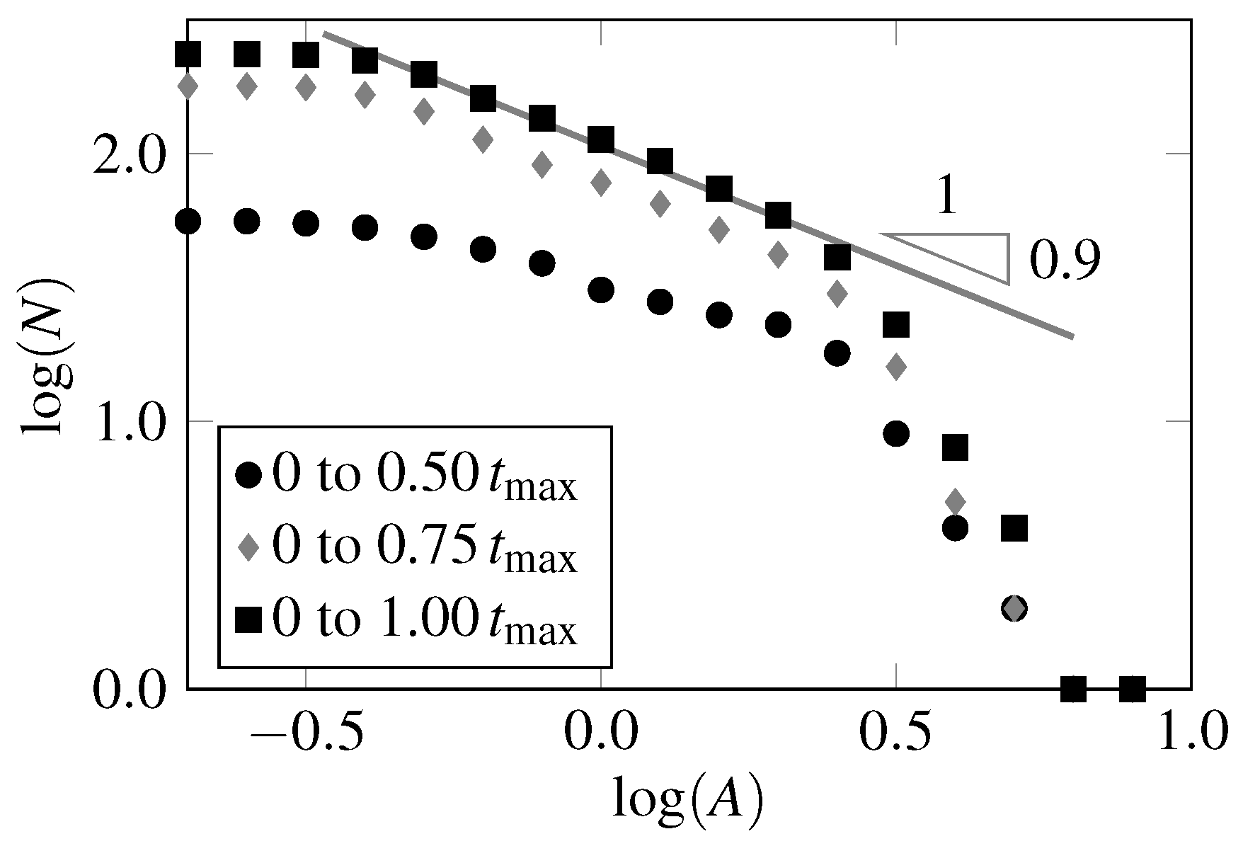
4.3. Comparison with the Bundle Model

Three histograms were computed to compare the AE-test results with the Bundle Model predictions: with the first 50% of observed signals, with the first 75% of signals, and with all signals. Figure 14 depicts the corresponding results. This information is complemented by Figure 15, which illustrates a typical acceleration pattern being observed throughout the tests. Because of measurement noise, a threshold $log\left(0.2\right)=-0.7$ is used for computing the AE-signals. In Figure 14, this implies the nearly horizontal distribution that was obtained for small amplitudes: as small avalanches are undistinguished from measurement noise, the counting of AE-signals remains constant.

Comparing the results in Figure 14 to the theoretical predictions that are given by the Bundle Model in Figure 6a,b, it is possible to observe that:

• The experimental results agree with the general shape predicted by the model, with a central part tending to a linear curve in the bi-log graph. This evidences that the damage process tends to occur according to an exponential function, but its characteristic exponent is different. The data are also consistent with the theoretically expected deviations towards both magnitude extremes.
• Reducing the sample size for drawing the distribution does not affect AE-events distribution only at the magnitude extremes: when only the first 50% of the data are used, the intermediate linear range reduces in amplitude, and the angular coefficient is also affected.
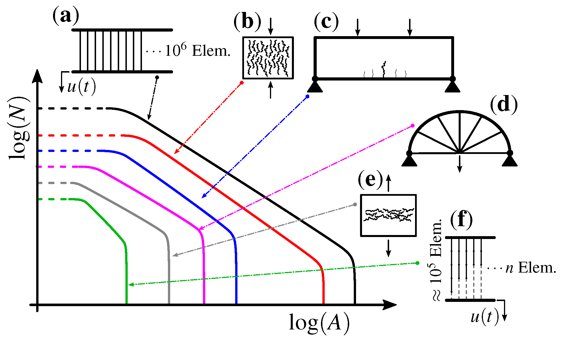
• The results that are presented here suggest that the damage process occurs according to a general pattern that is similar to the one predicted by the Bundle Model. However, this tendency suffers in varying degrees from the effects of measurement noise, the structure’s external geometry, the boundary conditions applied to it, and the internal organization of the system’s elements. The influence that is exerted by these factors is illustrated schematically in Figure 16. The two extreme cases correspond to the predictions given by the Bundle Model when all fibers are aligned in parallel (a) or almost entirely in series (f), whereas cases (b)–(e) represent several combinations of geometry and externally applied loads, which appear as intermediate arrangements within the context of the model. Thus, the spaghetti bridge configuration studied here is closer to the quasi-serial Bundle Model (case (f)), which is more prone to localization effects than the other cases. Finally, all profiles tend to a “platea” for small-amplitude events due to the need to apply a threshold value for negating measurement noise effects.

The following three examples reinforce the hypothesis presented in item (3):

(a)

In seismology [45,46] state that seismic events may result in any intermediate form between the extreme-case histograms depending on several characteristics of the region where the event occurs.

(b)

The behavior that is noted by [45] is also observed in the seismic behavior in the region of Angra dos Reis, Brazil, as evidenced by the corresponding histogram of seismic events shown in Figure 17.

(c)

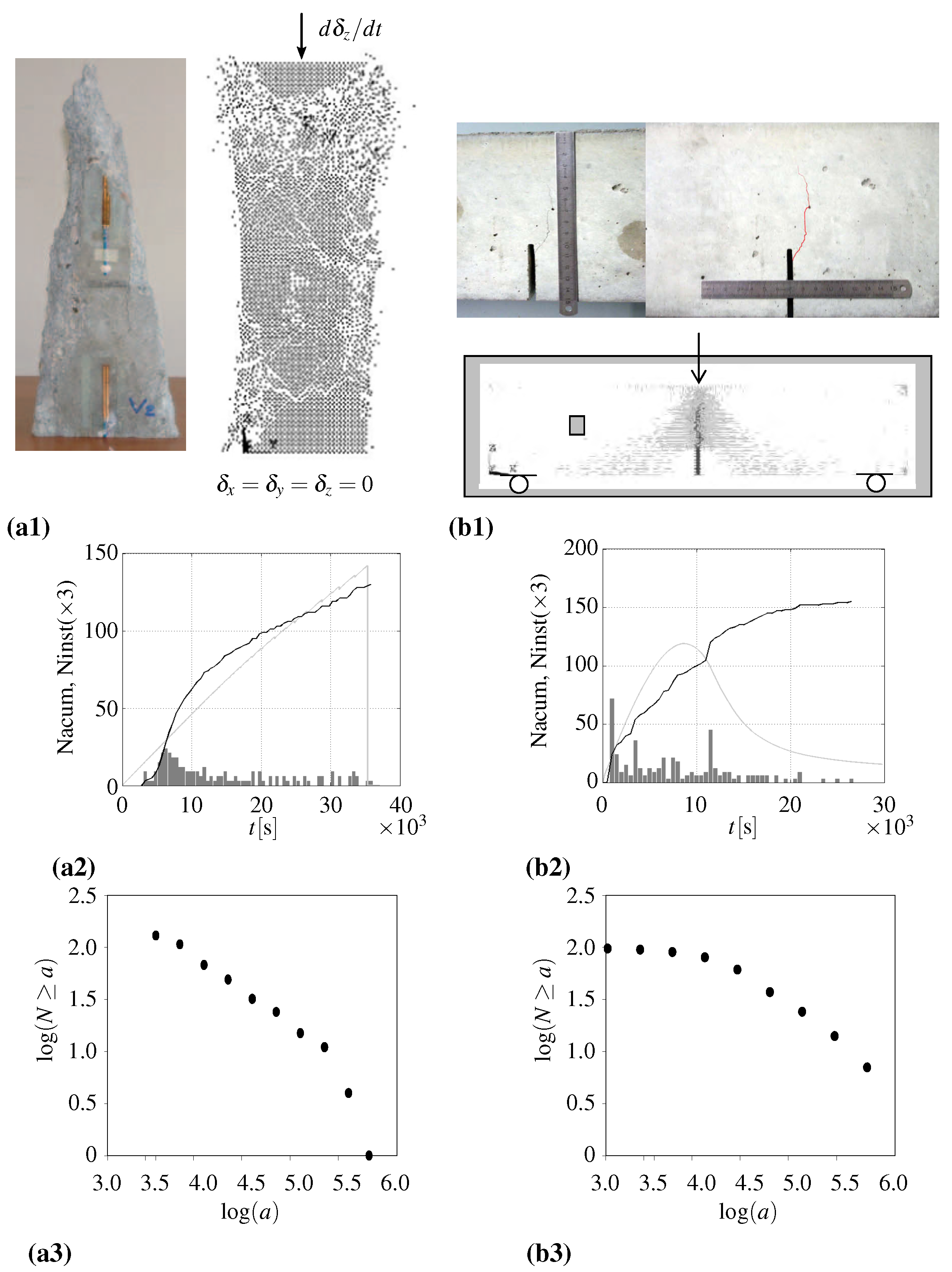
In [47], a comparative analysis is made between a prismatic specimen under uniaxial compression and a pre-fissured beam under flexion on three points. Both of the structures were made from concrete, and the comparison was carried out by both numeric and experimental means. The results are summarized in Figure 18, making it clear that geometry and boundary conditions significantly influence structural behavior. For instance, the histogram for the beam tends to horizontal for small magnitudes, because new ruptures tend to occur at the extremities of the pre-fissures, favoring the localization of avalanches and connection between events. As for the prismatic specimen, ruptures are equally likely to appear at every part of its structure in the initial phases, with localization only occurring for advanced stages of the damage process.

These three examples illustrate the possibilities of characterizing the damage process on different scales, from laboratory samples to seismic events. Other application examples also include in-situ large civil structures, such as in [48].

5. Conclusions

In this work, acoustic emission (AE) data were collected from a load test that was applied to a small-scale spaghetti bridge model, where the load increased until the structure collapsed. Four different parameters (b, $ϵ$, c, and $\gamma$) were computed from the AE data, and their usefulness in identifying damage progression was evaluated. The main conclusions from such a procedure are:

• The evolution of the coefficients b, $ϵ$, and c through time are suitable measures of the local instability that are associated with changes in the AE regime, with c (related with the event frequency distribution) being the most sensitive of the three.
• Computing $ϵ$ from the RMS-value of the AE signal yields improved sensitivity when compared to the traditional RILEM method.
• Analysis of frequency changes (variations in c and $\gamma$ coefficients) are useful not only for considering the isolated AE signals, but also the complete information collected by the AE sensors. In particular, the $\gamma$ coefficient presented a sharp reduction shortly before the localized damage became evident during the load test, which reinforces this coefficient’s usefulness as a failure predictor.
• The minimum values for coefficients c and $\gamma$ are consistent with the observations by Wilson [6] on the tendency of all phenomenon scales to participate when an instability occurs.
• When compared to the Bundle Model’s theoretical predictions, the experimental results presented here highlight the influence of boundary conditions, geometry, and internal organization on the collapse pattern of structures.

As a continuation of the present research, a Ph.D. thesis is ongoing at the Mechanical Postgraduate Program of Federal University of Rio Grande do Sul (PROMEC/UFRGS). The thesis work will include the study of AE signals from additional bridge models, such as the one used here, as well as other bridge geometries complying with the same contest’s guidelines, such as the limits for length and weight.

References

1. Krajcinovic, D. Damage Mechanics; North-Holland series. In Applied Mathematic and Mechanics; Elsevier: New York, NY, USA; Amsterdam, The Netherlands, 1996; ISBN 978-0-444-82349-6. [Google Scholar]
2. Biswas, S.; Ray, P.; Chakrabarti, B.K. Statistical Physics of Fracture, Breakdown, and Earthquake: Effects of Disorder and Heterogeneity; John Wiley & Sons: Weinheim, Germany, 2015; ISBN 978-3-527-41219-8. [Google Scholar]
3. Gao, H. A Theory of Local Limiting Speed in Dynamic Fracture. J. Mech. Phys. Solids 1996, 44, 1453–1474. [Google Scholar] [CrossRef]
4. Richter, C.F. Elementary Seismology; W. H. Freeman and Company and Bailey Bros. & Swinfen Ltd.: London, UK, 1958; Volume 2. [Google Scholar]
5. Turcotte, D.L.; Newman, W.I.; Shcherbakov, R. Micro and Macroscopic Models of Rock Fracture. Geophys. J. Int. 2003, 152, 718–728. [Google Scholar] [CrossRef] [Green Version]
6. Wilson, K.G. Problems in Physics with Many Scales of Length. Sci. Am. 1979, 241, 158–179. [Google Scholar] [CrossRef]
7. Rosser, J.B. The Rise and Fall of Catastrophe Theory Applications in Economics: Was the Baby Thrown Out with the Bathwater. J. Econ. Dyn. Control 2007, 31, 3255–3280. [Google Scholar] [CrossRef]
8. Hansen, H.F.; Hansen, A. A Monte Carlo Model for Networks Between Professionals and Society. Phys. Stat. Mech. Appl. 2006, 377, 698–708. [Google Scholar] [CrossRef]
9. Tainter, J.A. The Collapse of Complex Societies; New Studies in Archaeology; Cambridge University Press: Cambridge, UK, 1988; ISBN 978-0-521-38673-9. [Google Scholar]
10. Daniels, H.E. The Statistical Theory of the Strength of Bundles of Threads. Proc. R. Soc. Lond. A 1945, 183, 405–435. [Google Scholar] [CrossRef] [Green Version]
11. Hansen, A.; Hemmer, P.C.; Pradhan, S. The Fiber Bundle Model: Modeling Failure in Materials; Statistical Physics of Fracture and Breakdown; Wiley-VCH Verlag GmbH & Co. KGaA: Weinheim, Germany, 2015; ISBN 978-3-527-41214-3. [Google Scholar]
12. Riazi, A.; Karmo, D.; Shikh Ibrahim, M.A.; Amadou, S. Estimating the weight and the failure load of a spaghetti bridge: A deep learning approach. J. Exp. Theor. Artif. Intell. 2020, 32, 875–884. [Google Scholar] [CrossRef]
13. Acoustic Emission Testing; Grosse, C.; Ohtsu, M. (Eds.) Springer: Berlin/Heidelberg, Germany, 2008; ISBN 978-3-540-69895-1. [Google Scholar]
14. Carpinteri, A.; Lacidogna, G.; Corrado, M.; Di Battista, E. Cracking and Crackling in Concrete-Like Materials: A Dynamic Energy Balance. Eng. Fract. Mech. 2016, 155, 130–144. [Google Scholar] [CrossRef]
15. Hemmer, P.C.; Hansen, A. The Distribution of Simultaneous Fiber Failures in Fiber Bundles. J. Appl. Mech. 1992, 59, 909–914. [Google Scholar] [CrossRef]
16. Shiotani, T.; Fujii, K.; Aoki, T.; Amou, K. Evaluation of Progressive Failure Using AE Sources and Improved b-value on Slope Model Tests. In Proceedings of the Progress in Acoustic Emission Vii: Proceedings of the 12th International Acoustic Emission Symposium, Sapporo, Japan, 17–20 October 1994; pp. 529–534. [Google Scholar]
17. Aki, K. Scaling Law of Seismic Spectrum. J. Geophys. Res. 1967, 72, 1217–1231. [Google Scholar] [CrossRef]
18. Carpinteri, A.; Lacidogna, G.; Puzzi, S. From Criticality to Final Collapse: Evolution of the “b-Value” from 1.5 to 1.0. Chaos Solitons Fractals 2009, 41, 843–853. [Google Scholar] [CrossRef]
19. Carpinteri, A.; Lacidogna, G.; Niccolini, G. Fractal Analysis of Damage Detected in Concrete Structural Elements Under Loading. Chaos Solitons Fractals 2009, 42, 2047–2056. [Google Scholar] [CrossRef]
20. Han, Q.; Wang, L.; Xu, J.; Carpinteri, A.; Lacidogna, G. A Robust Method to Estimate the b-Value of the Magnitude-Frequency Distribution of Earthquakes. Chaos Solitons Fractals 2015, 81, 103–110. [Google Scholar] [CrossRef]
21. Iturrioz, I.; Lacidogna, G.; Carpinteri, A. Acoustic Emission Detection in Concrete Specimens: Experimental Analysis and Lattice Model Simulations. Int. J. Damage Mech. 2014, 23, 327–358. [Google Scholar] [CrossRef]
22. Ohtsu, M. RILEM Technical Committee (Masayasu Ohtsu) Recommendation of RILEM TC 212-ACD: Acoustic Emission and Related NDE Techniques for Crack Detection and Damage Evaluation in Concrete*: Test Method for Classification of Active Cracks in Concrete Structures by Acoustic Emission. Mater. Struct. 2010, 43, 1187–1189. [Google Scholar] [CrossRef] [Green Version]
23. Friedrich, L.; Colpo, A.; Maggi, A.; Becker, T.; Lacidogna, G.; Iturrioz, I. Damage process in glass fiber reinforced polymer specimens using acoustic emission technique with low frequency acquisition. Compos. Struct. 2021, 256, 113105. [Google Scholar] [CrossRef]
24. Kogan, S.M. Low-Frequency Current Noise with a 1/f Spectrum in Solids. Sov. Phys. Usp. 1985, 28, 170–195. [Google Scholar] [CrossRef]
25. Johnson, J.B. The Schottky Effect in Low Frequency Circuits. Phys. Rev. 1925, 26, 71–85. [Google Scholar] [CrossRef]
26. Milotti, E. 1/f Noise: A Pedagogical Review. arxiv 2002, arXiv:physics/0204033. [Google Scholar]
27. Lovejoy, S.; Schertzer, D. Scaling and Multifractal Fields in the Solid Earth and Topography. Nonlin. Process. Geophys. 2007, 14, 465–502. [Google Scholar] [CrossRef] [Green Version]
28. Kononovicius, A.; Ruseckas, J. Nonlinear GARCH model and 1/f noise. Phys. Stat. Mech. Appl. 2015, 427, 74–81. [Google Scholar] [CrossRef] [Green Version]
29. Dave, S.; Brothers, T.A.; Swaab, T.Y. 1/f Neural Noise and Electrophysiological Indices of Contextual Prediction in Aging. Brain Res. 2018, 1691, 34–43. [Google Scholar] [CrossRef] [PubMed]
30. Pease, A.; Mahmoodi, K.; West, B.J. Complexity measures of music. Chaos Solitons Fractals 2018, 108, 82–86. [Google Scholar] [CrossRef]
31. Voss, R.F.; Clarke, J. 1/f Noise in Music and Speech. Nature 1975, 258, 317–318. [Google Scholar] [CrossRef]
32. Mandelbrot, B.B. Fractals: Form, Chance, and Dimension; Freeman: San Francisco, CA, USA, 1977; ISBN 978-0-7167-0473-7. [Google Scholar]
33. Carpinteri, A.; Lacidogna, G.; Accornero, F. Fluctuations of 1/f Noise in Damaging Structures Analyzed by Acoustic Emission. Appl. Sci. 2018, 8, 1685. [Google Scholar] [CrossRef] [Green Version]
34. Peirce, F.T. Tensile tests for cotton yarns: “The weakest link” theorems on the strength of long and of composite specimens. J. Textile Inst. 1926, 17, 355–368. [Google Scholar]
35. Raischel, F.; Kun, F.; Herrmann, H.J. Fiber Bundle Models for Composite Materials. In Proceedings of the Conference on Damage in Composite Materials 2006, Stuttgart, Germany, 18–19 September 2006. [Google Scholar]
36. Boufass, S.; Hader, A.; Tanasehte, M.; Sbiaai, H.; Achik, I.; Boughaleb, Y. Modelling of composite materials energy by fiber bundle model. Eur. Phys. J. Appl. Phys. 2020, 92, 10401. [Google Scholar] [CrossRef]
37. Lehmann, P.; Or, D. Hydromechanical triggering of landslides: From progressive local failures to mass release: Hydromechanical Landslide Triggering. Water Resour. Res. 2012, 48, 535. [Google Scholar] [CrossRef]
38. Cohen, D.; Schwarz, M.; Or, D. An analytical fiber bundle model for pullout mechanics of root bundles. J. Geophys. Res. 2011, 116, F03010. [Google Scholar] [CrossRef] [Green Version]
39. Sornette, D. Elasticity and failure of a set of elements loaded in parallel. J. Phys. A Math. Gen. 1989, 22, L243. [Google Scholar] [CrossRef]
40. Okanagan College, Spaghetti Bridge Building Contest. Available online: https://www.okanagan.bc.ca/spaghetti-bridge (accessed on 20 February 2021).
41. Segovia González, L.A.; Morsch, I.B.; Masuero, J.R. Didactic Games in Engineering Teaching—Case: Spaghetti Bridges Design and Building Contest. In Proceedings of the 18th International Congress of Mechanical Engineering (COBEM 2005), Ouro Preto, MG, Brazil, 6–11 November 2005. [Google Scholar]
42. Competição De Pontes De Espaguete. Webmaster: Segovia González, L.A. Available online: https://www.ufrgs.br/espaguete/regulamento.html (accessed on 20 February 2021).
43. DTU Mechanical Engineering; DTU Compute TopOpt. Available online: https://www.topopt.mek.dtu.dk/ (accessed on 20 February 2021).
44. PCB Piezotronics, Inc. Model 352A60. High frequency, ceramic shear ICP®accel., 10 mV/g, 5 to 60kHz Installation and Operating Manual, 2nd ed.; PCB Group Inc.: Depew, NY, USA, 2008. [Google Scholar]
45. Bommer, J.; Stafford, P. Seismic Hazard And Earthquake Actions. In Seismic Design of Buildings to Eurocode 8; CRC Press: Boca Raton, FL, USA, 2016; pp. 7–40. [Google Scholar]
46. Riera, J.D.; Iturrioz, I. Performance of the Gutenberg-Richter Law in Numerical and Laboratory Experiments; IASMiRT: San Francisco, CA, USA, 2013. [Google Scholar]
47. Riera, J.D.; Iturrioz, I. Considerations on the Diffuse Seismicity Assumption and Validity of the G-R Law in Stable Continental Regions (SCR). Rev. Sul. Eng. Est. 2015, 12, 7–25. [Google Scholar] [CrossRef] [Green Version]
48. Carpinteri, A.; Lacidogna, G.; Invernizzi, S.; Accornero, F. The Sacred Mountain of Varallo in Italy: Seismic Risk Assessment by Acoustic Emission and Structural Numerical Models. Sci. World J. 2013, 2013. [Google Scholar] [CrossRef] [PubMed] [Green Version]
Figure 1. Basic setup for acquiring AE signals, with two AE sensors. Although both signals refer to the same event, they differ according to their positions along the structure.
Applsci 11 02718 g001
Figure 2. Typical AE signal with its parameters of interest.
Applsci 11 02718 g002
Figure 3. Precursors from AE tests, (a) obtaining b from Equation (1); (b) calculation of ϵ from Equation (2); and, (c) determining c from Equation (3).
Applsci 11 02718 g003
Figure 4. Relation between the power density spectrum and the frequency content, with calculation of the γ parameter.
Applsci 11 02718 g004
Figure 5. The Bundle Model. (a) Parallel bar model where a prescribed displacement u x is applied and the reaction P x is measured, (b) evolution of the load during the damage process in typical Bundle Model.
Applsci 11 02718 g005
Figure 6. The avalanches distribution in the Bundle Model, defining avalanche as the number of bars that break simultaneously. (a) When the prescribed displacement is continuously increased, but the test is stopped before complete failure (i.e., u x i < u x max ). (b) When u x is applied in discrete steps with amplitude δ u .
Applsci 11 02718 g006
Figure 7. Geometric restrictions for the University of Rio Grande do Sul (UFRGS) Spaghetti Bridge contest (adapted from [42]).
Applsci 11 02718 g007
Figure 8. Evolution of collapse loads for the UFRGS Spaghetti Bridge contestants, data from [42].
Applsci 11 02718 g008
Figure 9. A few winning designs for the UFRGS Spaghetti Bridge contest, data from [42].
Applsci 11 02718 g009
Figure 10. Damage progress over time for the studied Spaghetti Bridge.
Applsci 11 02718 g010
Figure 11. (a) Acoustic emission (AE) data acquired during the loading test, with illustrating signals from individual signals. (b) Load applied to the bridge with corresponding signal counts.
Applsci 11 02718 g011
Figure 12. Time evolution of value-b, value- ϵ and value-c.
Applsci 11 02718 g012
Figure 13. Evolution of γ throughout the AE test.
Applsci 11 02718 g013
Figure 14. N ( A ) —histograms from the AE— test results, taking into account 50%, 75%, and 100% of observed events.
Applsci 11 02718 g014
Figure 15. The acceleration pattern typically acquired during the tests, with the amplitude threshold that defined actual AE-signals.
Applsci 11 02718 g015
Figure 16. Frequency distribution of some measure of avalanches magnitudes in different structural typologies.
Applsci 11 02718 g016
Figure 17. (a) Distribution of epicenters of seismic events with M w 1.5 , recorded from 1959 to 2013 within a 1200 k m 2 area in South-Eastern Brazilian Stable Continental Regions (SCR). The red point shows the site of the Angra dos Reis NPP (CNAAA). (b) Relation between log ( n / N ) for the region during the same period [47].
Applsci 11 02718 g017
Figure 18. AE simulation results on concrete structures. (a) prism under uniaxial compression, (b) pre-fissured beam. (1) Results in terms of final configurations. (2) load vs time response (light-gray line), accumulated number of AE signals (dark line), and instantaneous distribution of events (histogram bars) (3) Accumulated number of signals vs. their magnitudes in bilogarithmic scale [46].
Applsci 11 02718 g018
Publisher’s Note: MDPI stays neutral with regard to jurisdictional claims in published maps and institutional affiliations.