Article

Global Solar Radiation Transfer and Its Loss in the Atmosphere

LAGEO, Institute of Atmospheric Physics, Chinese Academy of Sciences, Beijing 100029, China
*
Author to whom correspondence should be addressed.
Appl. Sci. 2021, 11(6), 2651; https://doi.org/10.3390/app11062651
Submission received: 11 January 2021 / Revised: 26 February 2021 / Accepted: 11 March 2021 / Published: 16 March 2021

Abstract

:
Based on the analysis of solar radiation and meteorological parameters measured at a subtropical forest in China during 2013–2016, a new empirical model of global solar irradiance has been developed. It can calculate global solar irradiance at the ground and at the top of the atmosphere (TOA); both are in agreement with the observations. This model is used to calculate the extinction of global solar irradiance in the atmosphere and the contributions from absorbing and scattering substances. The loss of global solar irradiance is dominated by absorbing and absorbing substances. The results show clear seasonal and interannual variations during the observation period. Sensitivity analysis indicates that global solar irradiance is more sensitive to changes in scattering, quantified by the S/G factor (S and G are diffuse and global solar radiation, respectively), than to changes in absorption. The relationships between the extinction factor (AF) of G and S/G and between the AF and the aerosol optical depth (AOD) are determined and used to estimate S/G and the AOD from the measured AF. This empirical model is applied to calculate the albedos at the TOA and the ground. This empirical model is useful to study global solar radiation and the energy–atmosphere interactions.

1. Introduction

Solar radiation in the atmosphere interacts with molecules and particles. It provides energy that drives the movement of air, convection, and advection. Solar radiation heats the atmosphere directly due to absorption by gases and aerosol particles and indirectly due to the conversion of solar radiation absorbed at the surface to long-wave outgoing radiation. This leads to the warming of the surface and the vertical and horizontal motion of the atmosphere. Therefore, it is important to study the transfer of solar radiation in the atmosphere and its extinction due to absorption and scattering by molecules and aerosol particles, in relation to their concentrations and meteorological variables, and thus understand the mechanisms in atmospheric physics and chemistry affecting climate and climate change and Earth’s energy budget [1,2,3,4,5,6,7,8].
Radiative transfer models (e.g., LOWTRAN and MODTRAN) are rigorous and sophisticated, and widely used for various applications, but require a large number of atmospheric parameters as input (e.g., gases, aerosols, and clouds), as well as assumptions and parameterizations. Therefore, less detailed empirical models are developed that require fewer input parameters obtained easily at ground stations. Many empirical models have been developed for estimating global, direct, and diffuse solar radiation at the ground [9,10,11,12,13,14,15,16,17,18], based on statistical relationships between radiation and parameters such as air temperature, relative humidity, atmospheric pressure, precipitable water, sunshine duration, visibility, altitude, latitude, clouds, atmospheric transmittance, and aerosol optical depth. A number of spectral and broadband models, such as Bird, REST, sSOLIS, MRM5, SMARTS, and others [9,10,11,12,13,14,15,16,17,18], are based on the mathematical representation of physical atmospheric processes (major extinction processes due to O3, water vapor, aerosol, NO2, etc.) and have good performance worldwide. These empirical models are formulated in linear, quadratic, cubic, logarithmic, exponential, power, and rational forms. Most of them were developed to estimate solar radiation at the surface for the study of solar radiation and the relation to climate, solar energy use, and site selection for solar photovoltaic plants [19]. However, it is not enough to study solar radiation only at the ground. Until now, it has not been reported that an empirical model can calculate global solar radiation at the top of the atmosphere (TOA), implying it is a challenging task. Moreover, using variables as less as possible to calculate global solar radiation is an effective method for saving computing cost. To better understand the atmospheric movement, energy budget, regional climate, and solar radiation at the surface and at the TOA, the extinction of solar radiation in the atmosphere due to absorption and scattering needs to be investigated. There is also a need to study the reflection and/or the albedo at the TOA and at the surface and the effect of solar radiation on climate change.
The objectives and main novelties of this study are to develop a new empirical model of global solar radiation based on the analysis of high-quality observational data under optimal atmospheric conditions and to further study (1) global solar radiation (hourly, daily, monthly, yearly) near the surface and at the TOA; (2) the extinction of global solar radiation in the atmosphere, associated with the total atmospheric absorbing and scattering substances (in the atmospheric column); (3) the albedo at the TOA and at the surface; and (4) relationships between both absorption and scattering and meteorological variables (temperature, relative humidity, and water vapor pressure). The achievement of these objectives is expected to improve our understanding of the basic processes and mechanisms associated with atmospheric radiation and its effect on regional climate and climate change. To achieve these objectives, four years of observations of solar radiation and meteorological parameters at a subtropical site in the south of China were analyzed, as described in Section 2.1. Observational data were used to develop an empirical model for global solar radiation, as described in Section 2.2. The model is applied to address the above objectives 1–3, and the results are compared with those from four other sites, in the north of China, in Section 3 and Section 4. The mechanisms underlying the production of OH radicals associated with water and water vapor in the UV and visible regions are discussed and emphasized.

2. Data and Methodology

2.1. Observations and Data Selection

Solar radiation and meteorological parameters were measured at the Qianyanzhou subtropical Pinus plantation, Taihe County, Jiangxi Province (26°44′48″ N, 115°04′13″ E, elevation 110.8 m), China, from 22 May 2013 to 31 December 2016. The solar radiation system consisted of three spectral radiation sensors (in the wavelength range of 270–3200, 400–3200, and 700–3200 nm, respectively, model TBQ-4–1) and a direct beam radiation sensor (270–3200 nm, model TBS). These radiation sensors were made by the 322 Institute of Jinzhou, China. All measurements were measured every second, including broadband global horizontal irradiance (GHI, referred to as G, 270–3200 nm) and direct normal irradiance (DNI, referred to as D, 270–3200 nm); UV and visible (VIS) irradiances were derived from the difference over 400–3200 nm, 700–3200 nm from 270–3200 nm, respectively; and near-infrared (NIR) irradiance was obtained from the measurement of 270–3200 nm. All sensors were installed on the roof of a building. Diffuse horizontal irradiance (DHI, in this paper referred to as S) was derived from the difference G- D × cos(Z), where Z is the solar zenith angle (in degrees). The yearly non-stability of the global solar radiation sensor is <±2%, the temperature dependence is 0.05% per degree, and the cosine response error is ≤±3% for a solar zenith angle of <70°. The annual non-stability of the solar direct radiation sensor is <±1% per year, its tracking accuracy is <±1°/24 h, and the ambient temperature range is <±45 °C. All solar radiation sensors were cleaned every morning before sunrise and, when necessary, during the daytime, e.g., after rain. All sensors were calibrated before this campaign and calibrated regularly (1 or 2 years) using Eppley radiometers (Model PSP) with WG 295 and WG 395 filters, respectively. The solar radiation system and the sensor calibration are described in detail in [20]. Global and direct radiation sensors were calibrated using a reference instrument that is traceable to the Chinese national radiometric reference [20]. The desiccant of all sensors was replaced when the color of the silica gel drying agent changed to pink. Meteorological conditions near the surface were measured using a HOBO weather station (Model H21, Onset Company, Bourne, MA, USA). Temperature, humidity, water vapor, and cloudiness (N, from 0, cloud free, to 1, overcast) were recorded.
In total, 19,014 hourly radiation data items (global, direct, UV, VIS, NIR) passed quality control criteria, together with meteorological variables (temperature, humidity, water vapor), and were used in the analysis from the measurements at Qianyanzhou Station between 1 January 2013 and 31 December 2016, i.e., hourly radiation (global without direct normal radiation), and meteorological data during 1 January–22 May 2013 were obtained from the Qianyanzhou Experimental Station of the Chinese Academy of Sciences (CAS); thereafter, measurements were continued by the Institute of Atmospheric Physics (IAP). The 19,014 hourly observational data items were used for daily and monthly averages in later analysis.
To ensure that only good-quality solar radiation data were used to compute the daily and monthly values in this study, data measured early in the morning and in the late afternoon (i.e., within 1 h from sunrise and sunset) were excluded because of the low solar elevation angle resulting in large cosine errors. In addition, extreme values of irradiance (G, S, D) and the S/G ratio (dimensionless) were excluded because they could be due to events such as heavy rain, dense haze, or dew, and water droplets on the windows of the radiation sensors could cause large observational errors. Values for global and direct solar radiation larger than extraterrestrial radiation were not observed. This data quality corresponds to that using the observed solar radiation data in the range of 0–1.2 times the extraterrestrial radiation by Bilbao et al. [21].

2.2. Model Formulation

Global solar radiation at the ground is determined by the position of the sun and the extinction by atmospheric gases, liquids, and particles (GLPs). The principle of energy balance in the UV and VIS regions (290–400 and 400–700 nm, respectively) has been applied to data obtained from 4 sites in the North of China [20,22]. For the further application of the same method to the observations at the Qianyanzhou subtropical site in the short-wavelength region (270–3200 nm), two key processes associated with global solar radiation transfer in the atmosphere are considered:
1.
The absorption term: absorption and use of global solar radiation by GLPs, including:
(a)
GLPs at wavelengths in the 290–400 nm region, when they participate in chemical and photochemical reactions (CPRs), with emphasis on volatile organic compounds (VOCs) through OH radicals and H2O
(b)
GLPs at wavelengths in the 400–700 nm region, when they participate in CPRs through OH radicals and H2O
(c)
H2O and other GLPs at wavelengths in the near-infrared (NIR) region (700–3200 nm)
A detailed introduction to OH production mechanisms at wavelengths in the UV and visible regions is given in [22,23,24,25,26,27] and the references in these papers. The fraction of global solar radiation absorbed by water vapor in the wavelength region of 0.70–2.85 μm is expressed as S’ = 0.17 (mW)0.30 [28]; the total water vapor content in the atmospheric column (cm), W = 0.02E × 30 [22]; and E is the average water vapor pressure (hPa) at the ground. If only water vapor is considered and the atmosphere is plane-parallel, the solar radiation on the horizontal surface can be described as
I0 cos Z − ΔS’= I0e−kWm × cos(Z)
e−kWm=1 − ΔS’/Io
where I0 = 1.94 cal min−1 cm−2 (=1367 W m−2) is the solar constant, k is the average absorption coefficient of water vapor in 0.70–2.85 μm, and m is the optical air mass in the middle of each hour. The absorption term at the horizontal plane is expressed as ekWm × cos(Z).
2.
The scattering term: Scattering of solar radiation by GLPs in the atmosphere is assumed to vary exponentially with S/G, i.e., e−S/G, where S/G is a normalized parameter that objectively represents the total scattering by atmospheric GLPs in the atmospheric column, including molecules, particles, clouds, haze, and water vapor [22].
The hourly global solar irradiance under all-sky conditions was calculated by an empirical model:
G cal   =   A 1 e kWm   ×   cos ( Z )   +   A 2 e S / G obs +   A 0
where the subscripts cal and obs refer to calculated and observed hourly values of G and S and are expressed in MJ m−2. Coefficients A1 and A2 (MJ m−2) represent the modulating roles of the individual absorption and scattering terms in Gcal at the TOA, and A0 (MJ m−2) indicates the reflected irradiation at the TOA. A1 and A2 indicate the solar irradiation at the TOA corresponding to the absorption and scattering terms, respectively. In other words, the solar radiation is absorbed and scattered by the atmospheric GLPs, and these processes are described by A1, A2, and A0 at the TOA and absorption and scattering terms in the atmosphere, respectively. The sum of A1, A2, and A0 is the total solar irradiation at the TOA. It is also easily calculated using the solar constant and the Earth–sun distance and is used to evaluate empirical model performance. The contributions of the absorption and diffuse terms (i.e., A1, A2) to G under realistic atmospheric conditions were quantified by fitting the observed G and absorption and diffuse terms (Equation (3)).

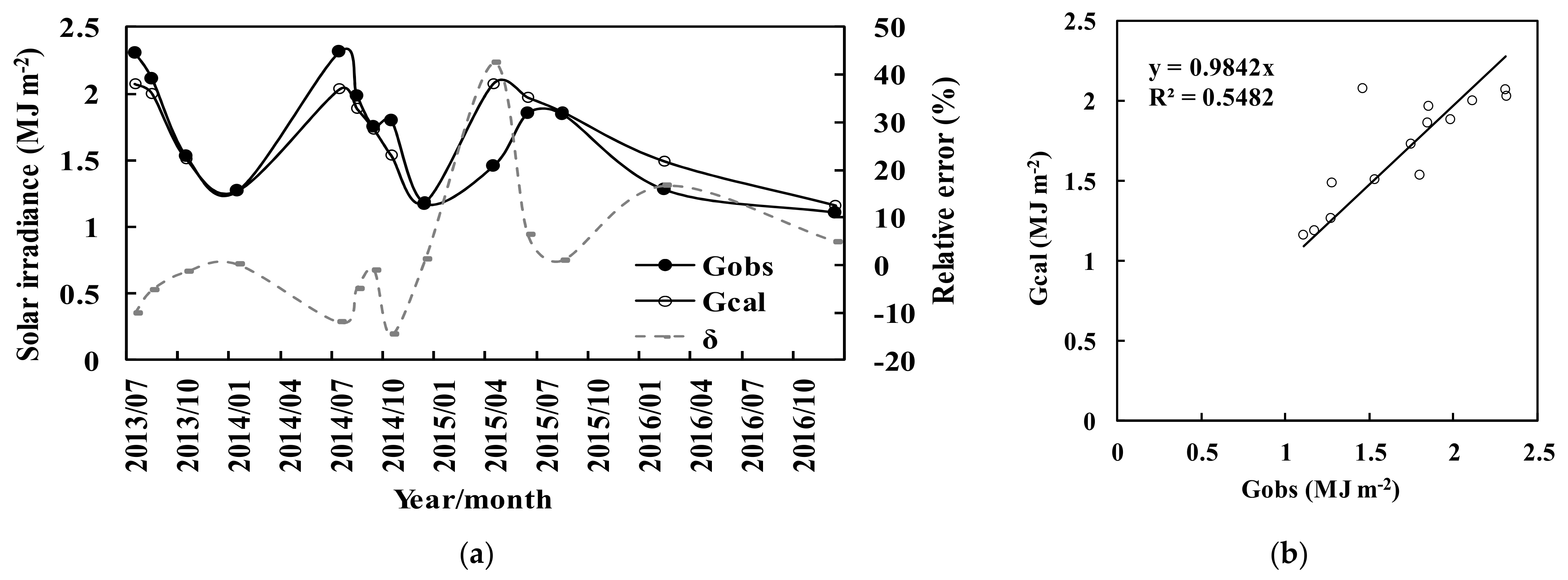
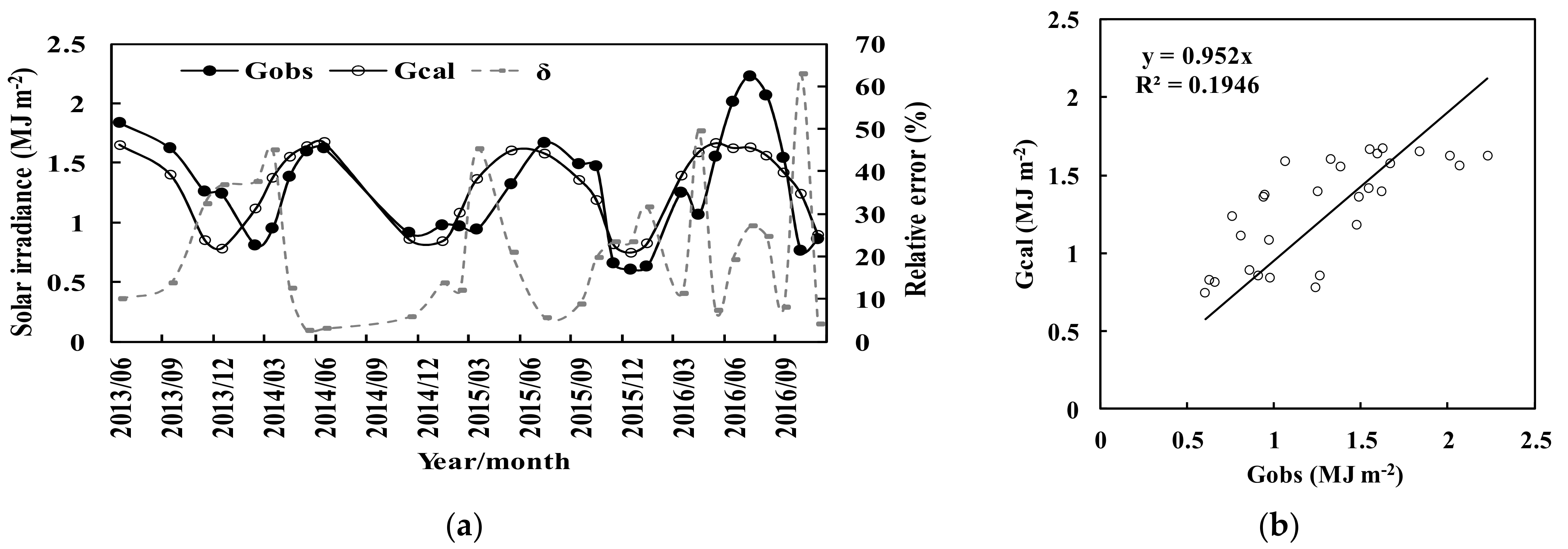
2.3. Determination and Evaluation of Model Coefficients for the Qianyanzhou Subtropical Site

To develop a reliable and optimal empirical model, i.e., the model coefficients Ai, only high-quality data were selected following the criteria described in Section 2.1, together with stricter criteria: (1) observations during early morning and late evening were excluded in order to decrease the influence of cosine errors of radiation sensors when Z was larger than 70° (i.e., solar radiation data at 9:00–16:00 local time were used), and (2) data with S/G of ≥0.80 and N of >0.80. Hourly averaged solar irradiance and meteorological variables (e.g., E) were calculated for each hour from 9:00 to 16:00, and these hourly averages were used, in turn, to calculate daily averages. Then, the corresponding monthly mean values were obtained from the daily averages. This resulted in 14 months of high-quality data (n = 14), corresponding to 397 daily and 2779 hourly data sets used for model development. To further reduce the random errors in the measurements and model development, monthly mean data were used in the development of the empirical model (Equation (3)), instead of hourly data.
The coefficients Ai in Equation (3) were determined using a multi-parameter fit. The results are presented in Table 1, i.e., the coefficients (A1, A2, A0) in Equation (3) as well as the coefficient of determination (R2) and the mean absolute value of the relative error (δavg) between calculated and measured G. The normalized mean-square error (NMSE), the mean absolute deviation (MAD, in exposure units, MJ m−2, and in percentage of the mean experimental value, %), and the root-mean-square error (RMSE, in exposure units and in percentage of the mean experimental value) are also included in Table 1. The calculated and observed solar irradiances and their relative errors (δ) are presented in Figure 1a as time series, and the calculated solar irradiances were evaluated versus the observed values in the scatterplot in Figure 1b. The slope of the linear regression of Gcal on Gobs (forced through zero) was 0.98, with a coefficient of determination R2 of 0.55 (different from the R2 in Table 1, because different equations were used, i.e., linear regression and Equation (3)). The data in Figure 1b show that the calculated G is in agreement with the observed values under all-sky conditions. The albedo at the TOA during 2013–2016 was 17.49%, which was estimated using |A0|/(A1 + A2 + |A0|).
The multi-parameter statistical analysis showed a strong correlation between G and the absorption term e−kWm × cos(Z) (at the confidence level α = 0.001), whereas the correlation between G and the scattering term e S / G obs (α = 0.001) was weak, i.e., absorption had a stronger influence on the global solar irradiance G than scattering. In addition, the correlation between e−kWm × cos(Z) and e S / G obs (α = 0.001) was not strong, i.e., the absorbing and scattering terms were independent, indicating that the absorption term can describe total absorption caused by all GLPs, independent of the scattering term, and vice versa. The value of the RMSE (Table 1) (e.g., 0.23 for S/G < 0.80) was in good agreement with the average value of 0.22 calculated using 7 empirical models with better performance out of 105 models [17], indicating reliable performance using the empirical model.
To investigate solar radiation under atmospheric conditions with S/G ≥ 0.80, e.g., under heavy fog and cloud cover conditions, N > 9/10, the relevant monthly observational data (n = 29) were analyzed using the same method as above, and an equation was determined similar to Equation (3). The main results are shown in Table 1 and Figure 2a,b. This situation may represent severe smog or heavy air pollution in other sites, so it is necessary to investigate solar radiation, its transfer, and its distribution in the atmosphere.
In general, the estimated G under these conditions correlated with that obtained directly from the observations but with larger uncertainties, i.e., larger δavg, δmax, MAD, and RMSE. It is noted that the uncertainties for various broadband solar radiation models are within 20% [14].
The albedo at the TOA under conditions with S/G > 0.80 in 2013 to 2016 was 24.48%, i.e., larger than that (21.19%) under conditions when S/G < 0.80, indicating that higher concentrations of atmospheric components (S/G) resulted in larger reflection at the TOA. Furthermore, such higher concentrations led to an increase in the extinction of G at the surface by 24.23% (the monthly mean values of G for S/G < 0.80 and S/G ≥ 0.80 were 1.70 and 1.29 MJ m−2, respectively).

3. Results

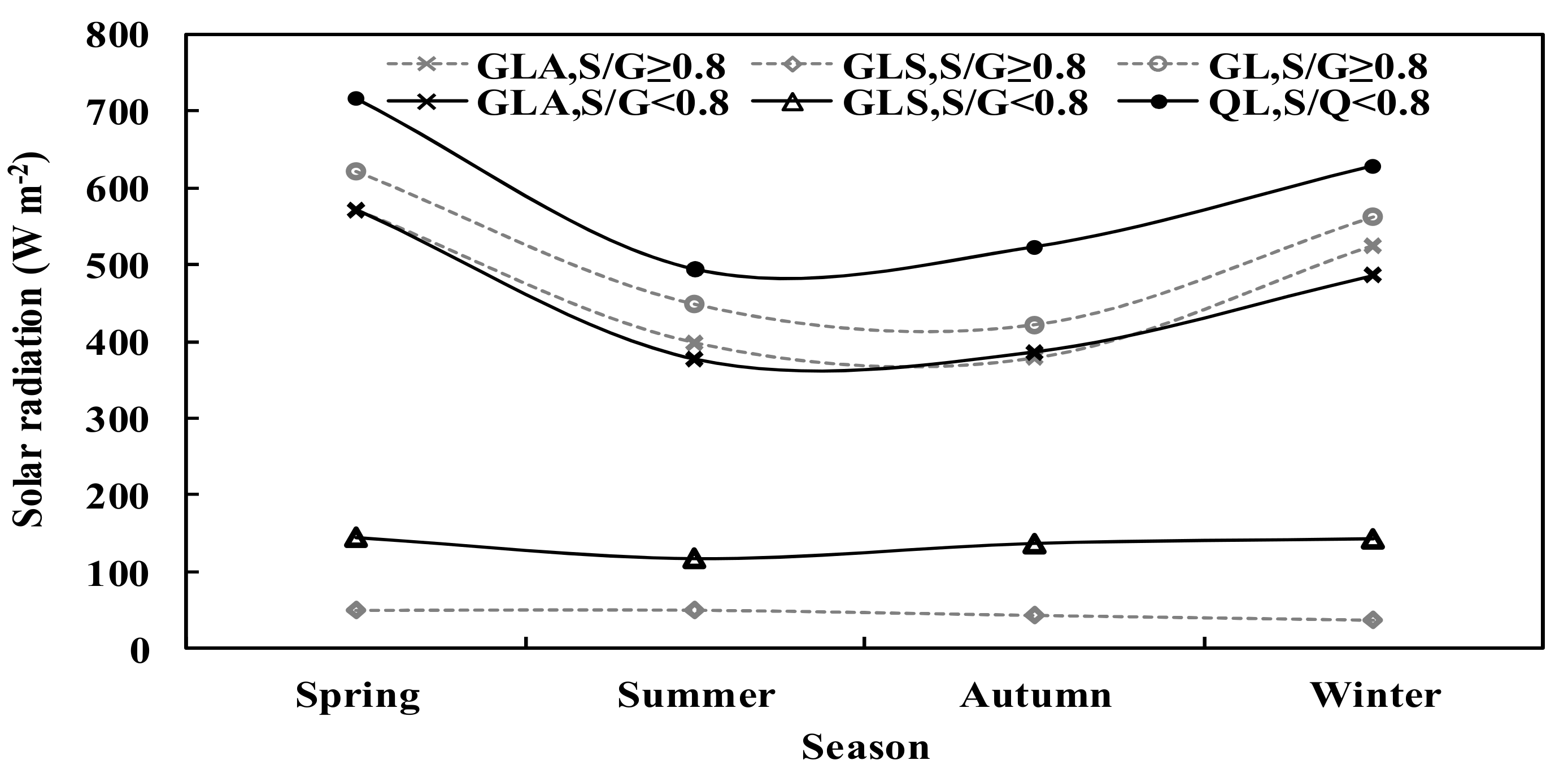
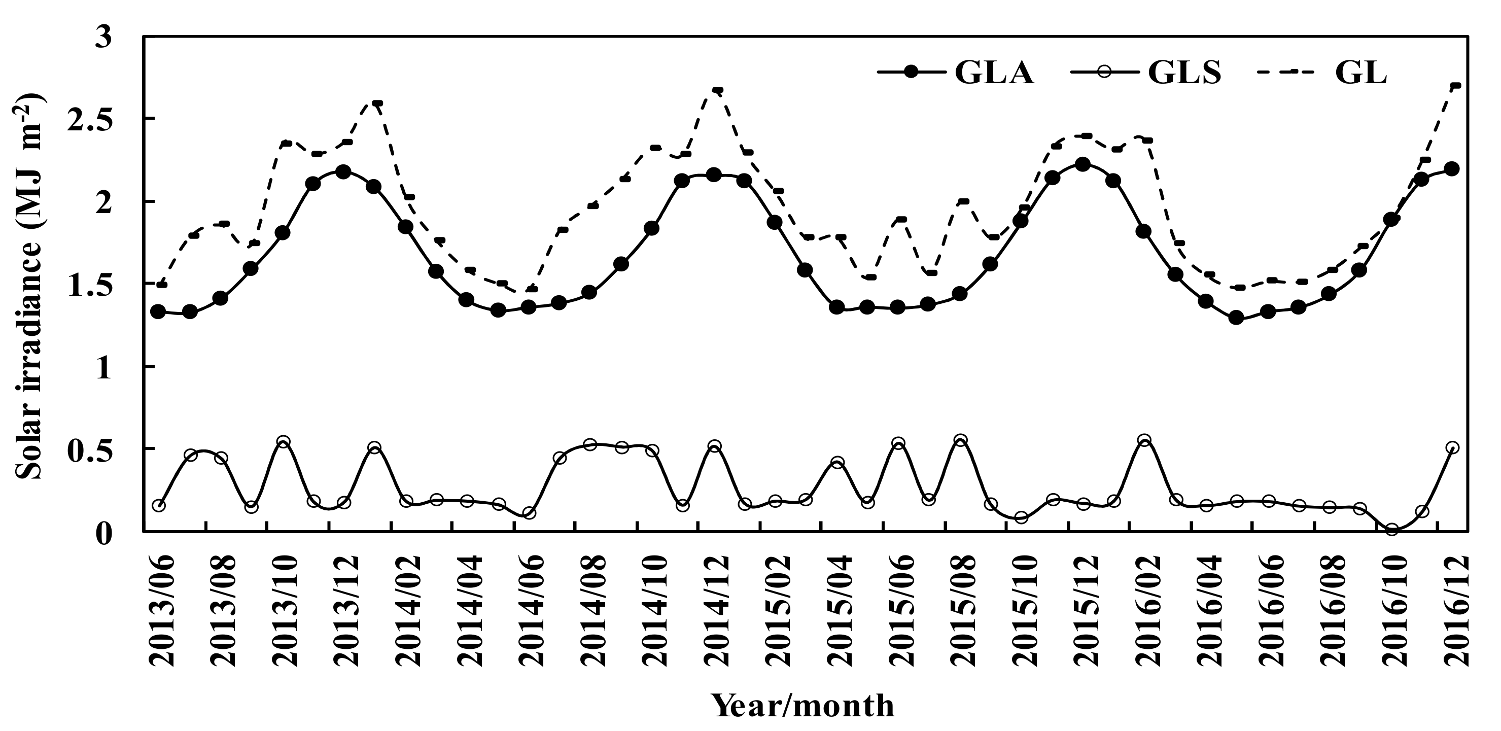
3.1. Seasonal Variation in Global Solar Irradiance Losses Due to GLP Extinction

Monthly losses of global solar irradiance attenuated by absorbing and scattering GLPs were calculated using the absorbing and scattering terms in Equation (3), further referred to as GLA (=A1(1 − e−kWm × cos(Z)) and GLS (=A2(1 − e S / G obs )), respectively. Based on the monthly values, seasonal mean losses averaged over the period 2013–2016 were determined for both S/G < 0.80 and S/G ≥ 0.80. The annual mean values of monthly water vapor and S/G were also calculated for these two atmospheric situations. The results are presented in Table 2 and Table 3 and in Figure 3.
GLA clearly varied with the seasons (e.g., higher in spring and lower in summer), for both atmospheric conditions (S/G < 0.80 and S/G ≥ 0.80). In contrast, GLS had a similar value in all seasons, although the values for S/G < 0.80 were somewhat higher in spring and winter and the values for S/G ≥ 0.80 were somewhat higher in spring and summer. Because GLA was much larger than GLS, the seasonal variation in GL was determined by that of GLA, i.e., absorbing processes and absorbing GLPs.
Comparison of the annual averages for both situations in Table 4 and Table 5 showed that for S/G ≥ 0.80, the annual GLA was only a little larger than for S/G < 0.80; in contrast, the annual GLS was a factor of 3 smaller. Hence the annual GL was somewhat lower for S/G ≥ 0.80 than for S/G < 0.80. The difference in annual loss was largely influenced by the scattering, i.e., the larger scattering loss was caused regional scattering aerosols in a relatively clean atmosphere than a polluted atmosphere. These differences were associated with a large increase in the annual atmospheric GLPs (S/G, 27.89%) and a slight decrease in water vapor (−10.79%), and the corresponding scattering and absorbing loss rates were 66.67% and 1.81%, respectively. The mechanisms underlying these differences were revealed in the sensitivity test (Section 3.4).
For situations with both S/G < 0.80 and S/G ≥ 0.80, GLA was much larger than GLS, but the relative contributions of GLA and GLS to GL were similar in each season. In other words, the extinction of global solar radiation over the Qianyanzhou subtropical forest region was mostly dominated by absorbing substances in four seasons, especially in high GLP loads.

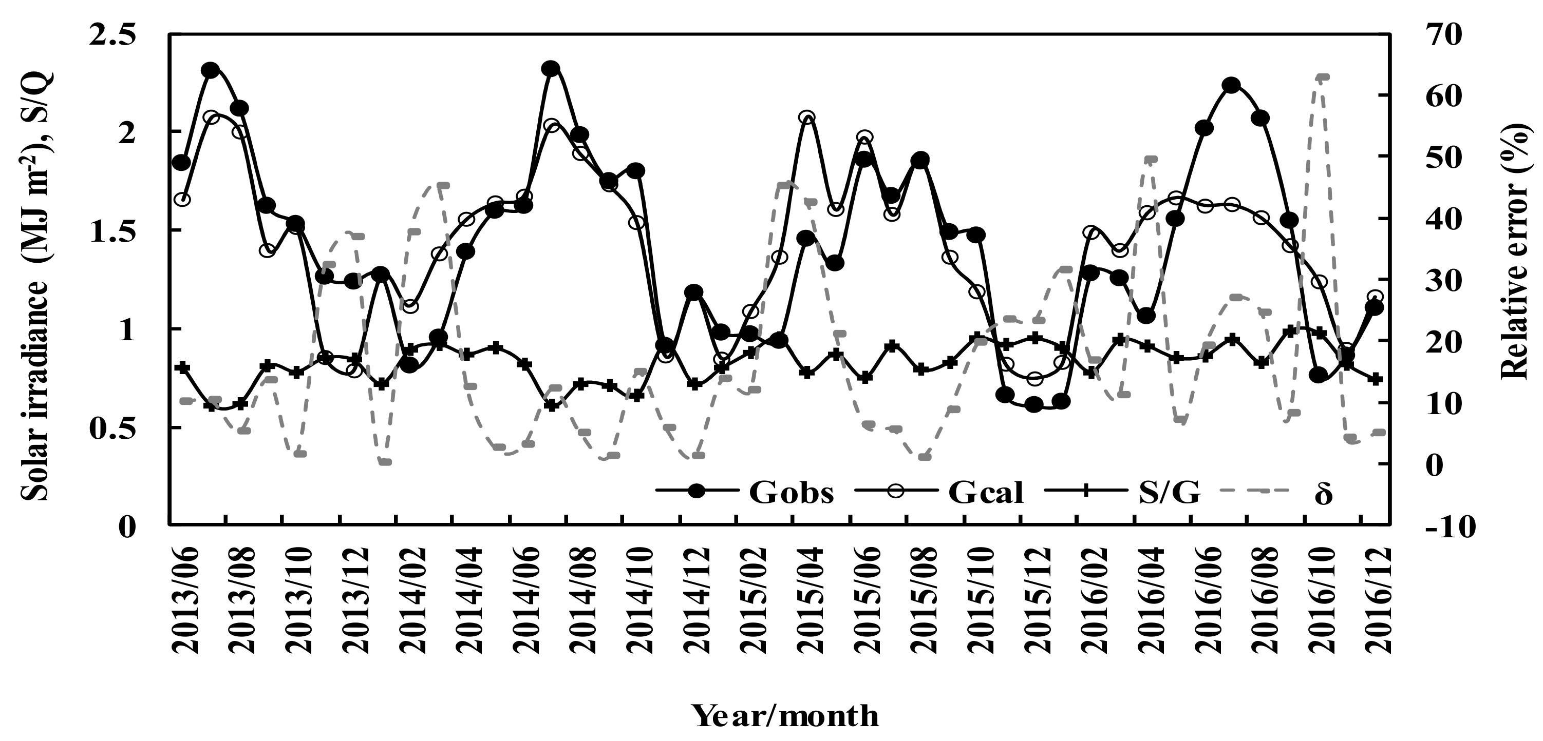
3.2. Variations in Global Solar Irradiance and Their Losses in the Atmosphere

Combining the above monthly observational data (n = 43) and corresponding calculated values for situations with S/G < 0.80 and S/G ≥ 0.80, time series of monthly mean global solar radiation and their losses in the atmosphere were obtained. The results are presented in Figure 4 and Figure 5. Figure 4 shows the time series of calculated and observed monthly means of global solar irradiances and their relative errors, and S/G from June 2013 to December 2016. The estimated and observed global solar irradiances under all-sky conditions were in good agreement, although larger relative errors appeared in situations with high S/G. This may be due to enhanced observational and calculation errors under these conditions. The observed and calculated time series showed an overall decrease of −3.62% per year and −2.58% per year, respectively. The increase in atmospheric substances (i.e., S/G) is one of the main reasons for the decrease in global solar irradiance, in good agreement with the earlier observation that “increasing aerosol loading is responsible for the observed reduced global solar radiation” [29] (Yang et al., 2019). The decrease in global solar irradiance led to a solar dimming in this subtropical region in China. Yang et al. [29] also showed a similar decrease in global solar radiation under all-sky conditions in Jiangxi Province during 2008–2016. Sogacheva et al. [30] showed that the aerosol optical depth (AOD) decreased over Southeast China in 2011–2017, and the difference between the AOD and S/G may be due to the difference in space and time match. It should be mentioned that the solar radiation sensors were calibrated before this study and daily maintenance was carried out during 2013–2016 (Section 2.1).
Monthly mean losses of the global solar irradiance during June 2013 to December 2016 were calculated, and the results are presented in Figure 5. The losses due to absorption, GLA, which dominate the total loss GL, as mentioned above, showed clear seasonal variations, higher in winter and lower in summer, corresponding to the higher water vapor pressure (together with higher other GLPs, NOx, SO2, O3, particulate matter (PM), etc.) [31] in winter and lower water vapor pressure in summer (Table 2 and Table 3), whereas there was no apparent seasonal variation in GLS, where most peaks appeared during June to October and in winter. During June 2013 to December 2016, GLA increased slightly, by 0.01% per year, associated with the increase in water vapor pressure by 0.50% per year (our measurement). This implies an increase in absorbing GLPs, including absorbing aerosols in the UV, VIS, and NIR regions, e.g., gases, secondary organic aerosols (SOA) produced from photochemical reactions of biogenic volatile organic compounds (BVOCs) through OH radicals [20,22,25,32,33,34,35,36,37]. GLS decreased by 9.71% per year, associated with the increase in S/G by 6.08% per year. GL decreased by 1.72% per year. The increase in S/G (Figure 4) indicated the increase in atmospheric GLP concentrations, resulting in a decrease in G at the ground and an increase in reflection at the TOA. This is deduced from the higher albedo of 25.48% for S/G ≥ 0.80 as compared to the albedo of 21.19% for S/G < 0.80. Following a method similar to that used in the empirical model development, the re-analysis of the monthly data for each year showed that the albedos from 2013 to 2016 were 19.50%, 22.41%, 23.64%, and 24.43%, respectively. These values correspond well with the annual values for S/G of 0.76, 0.79, 0.86, and 0.88, respectively.

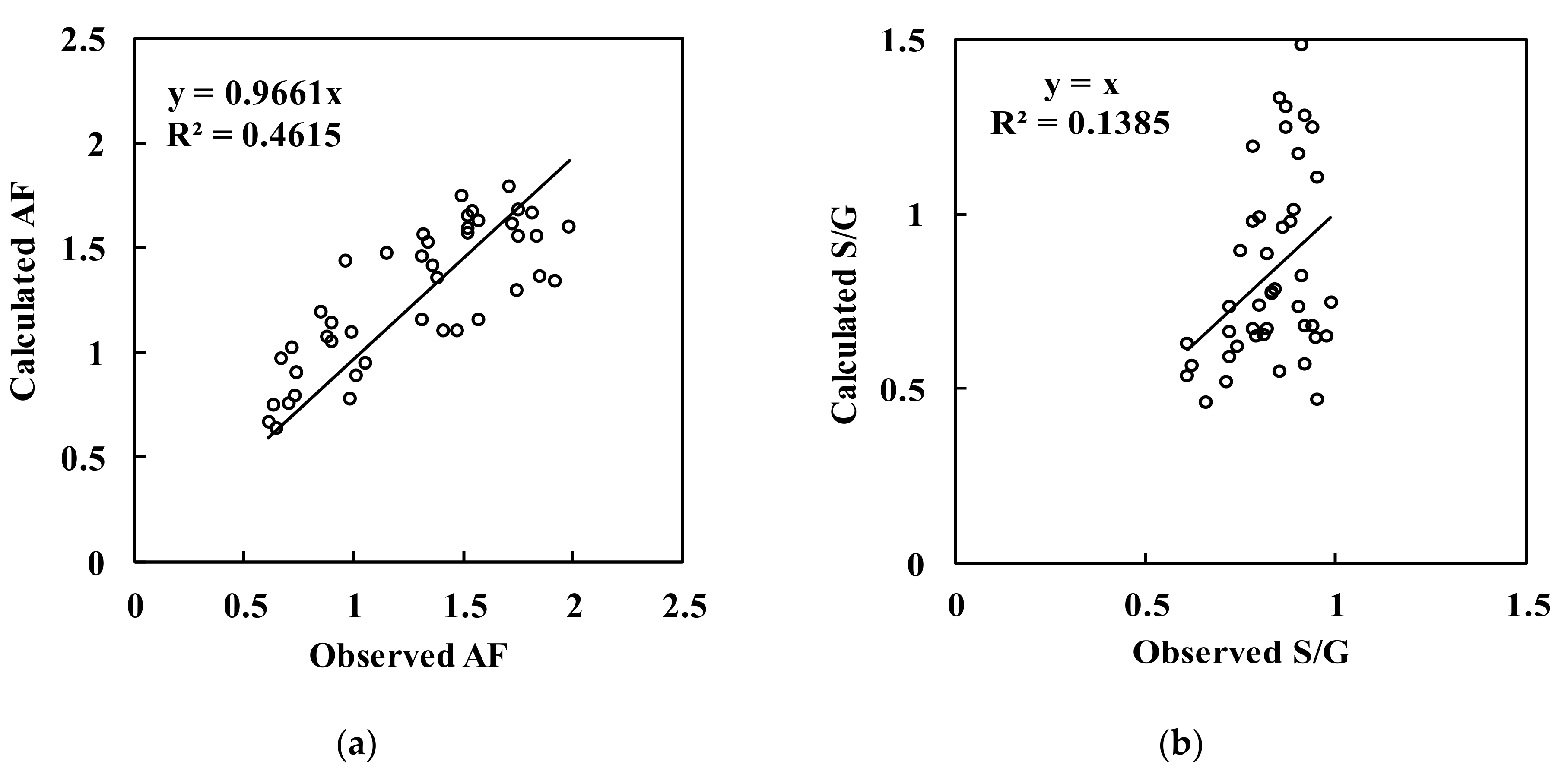
3.3. Extinction Factor and Related Estimation of Solar Radiation

Considering that direct global solar radiation is observed at a limited number of sites in China, a method is proposed to calculate S/G. The method is based on the evaluation of an extinction factor (AF), which is formulated as follows:
AF = (1 − (Gi/cos(Z)-GDmax))/(GDmax/GMmax)/(GMmax/GYmax)/(GYmax/G4Ymax)
where Gi is the observed global solar irradiance G for each hour i; GDmax, GMmax, and GYmax are the maxima of G for each day, month, and year, respectively; and G4Ymax is the maximum of G during four years (2013–2016).
The AF contains information about the extinction of solar radiation due to both absorbing GLPs (expressed as water vapor pressure, E) and scattering GLPs (expressed as scattering factor, S/G) in the atmosphere. Therefore, relationships between the AF and water vapor pressure and S/G were investigated. To fully understand the performance of Equation (4) and the AF under two atmospheric conditions, S/G < 0.80, which is the most representative, and S/G ≥ 0.80, with high concentrations of GLPs, all data observed during 2013–2016 were used.
Multiple regression analysis provided the following relationship between the AF and water vapor pressure and S/G (n = 43, all monthly data):
AF = 0.04 × E + 1.00 × (S/G) − 0.41
The calculated and observed AFs compared favorably, as shown in Figure 6a; the statistical metrics were R = 0.801, α= 0.001, δavg = 16.71%, and δmax = 40.81%. Monthly data in May 2013 were not used in the analysis, because the observations started on 22 May 2013. Then, S/G was calculated by application of Equation (5), with the AF calculated from Equation (4) (δavg = 23.63%, δmax = 63.04%), and the scatter plot of the calculated versus the observed values for S/G is presented in Figure 6b. Using these new estimates of S/G, the global solar radiation at the ground and the loss in the atmosphere were estimated for S/G < 0.80 and S/G ≥ 0.80 situations. Note that Equation (5) and the equations in Figure 6 for the AF and S/G are not the same. Equation (5) was used to estimate the AF and S/G and their relative biases (e.g., δavg, δmax), which subsequently were compared to the observed values in Figure 6.
A detailed summary of the results obtained using the AF to calculate annual mean losses is provided in Table 4. For comparison, annual mean losses calculated using the observed S/G values (e.g., observed S to observed G) are given in Table 5. Comparison of the data in Table 4 and Table 5 showed that the results from using the AF method were close to those using observed S/G values from observations of S and G. In general, the seasonal and annual mean losses (GLA, GLS, GL) calculated using the AF method were close to those using observed S/G values for both S/G < 0.80 and S/G ≥ 0.80. In addition, GLA, GLS, and GL varied in seasonal and annual patterns similar to those using observed S/G values.
We thus conclude that for cases when solar direct radiation measurements or the S/G factor are not available, the losses of global solar radiation can be estimated using the AF method. In addition, an empirical model of global solar radiation using the AF instead of S/G is suggested (Table 4, Table 5 and Table 6). AF values can easily be obtained from routine measurements of hourly global solar irradiance (Equation (4)).
Table 6 provides a detailed comparison of the averages over all months in 3 years of global solar irradiance, absorbing and scattering irradiances, and related parameters, calculated using S/G obtained using the AF method and that obtained from observations of S and G. The results showed that most corresponding calculated solar radiation parameters were similar. So, the AF-based S/G method can be used for estimation of global solar irradiance at the ground.

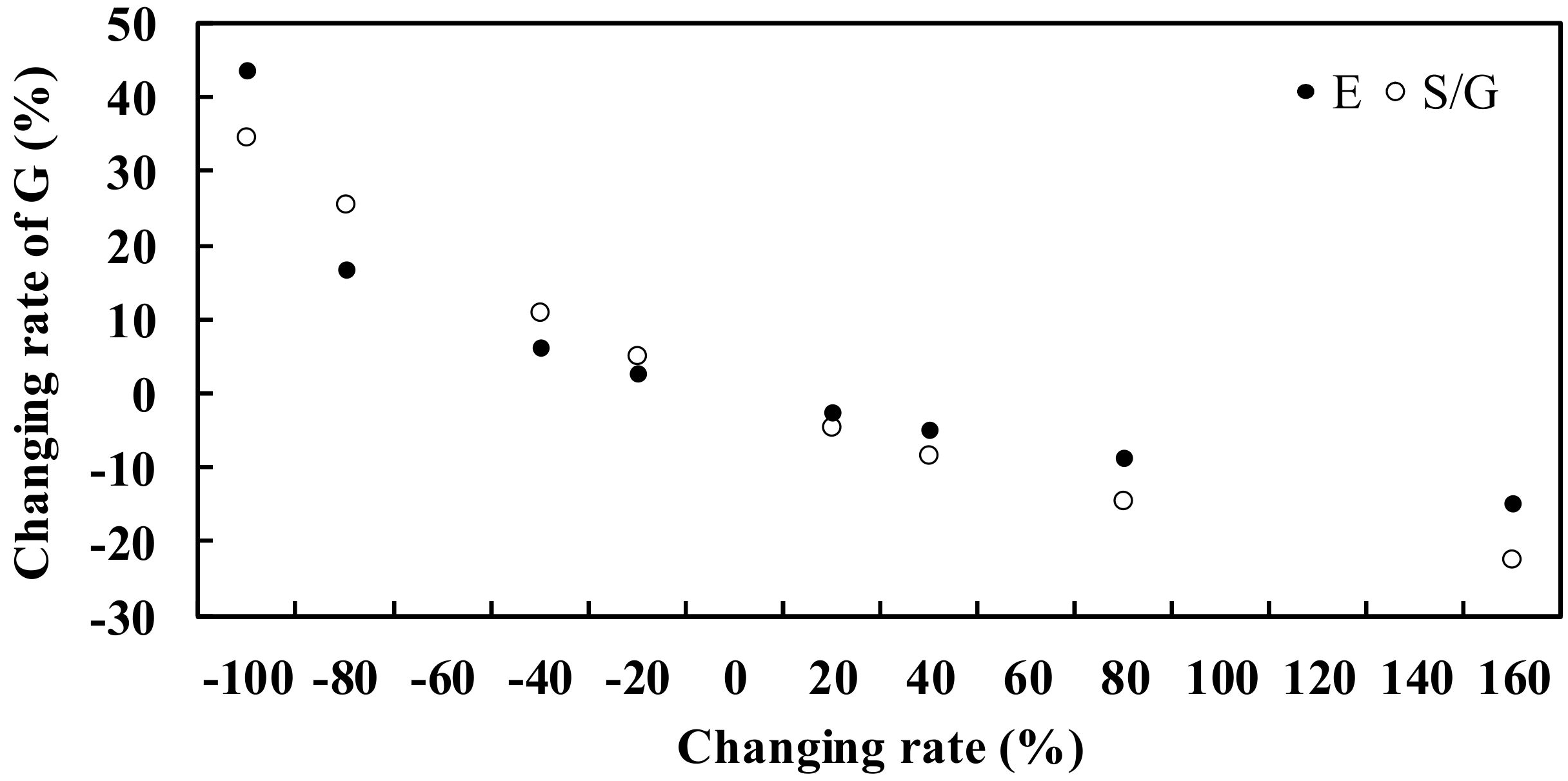
3.4. Sensitivity Test

The response of global solar irradiance to changes in total column absorbing or scattering substances (represented by E and S/G, respectively), i.e., the response of global solar irradiance to a change in one factor, while keeping other factors fixed, was studied using Equation (3). The atmospheric conditions of S/G < 0.80 were selected for this test. The results are presented in Figure 7 and Table 7.
The hourly global solar irradiance at the ground decreased/increased with the increase/decrease in water vapor pressure, indicating that increasing concentrations of highly absorbing GLPs (e.g., NOx, SO2, O3, BVOCs, SOA, OC) result in increased loss of solar irradiance and thus lower irradiance at the ground. Similarly, global solar irradiance decreased/increased with an increase/decrease in atmospheric GLPs (S/G used as an indicator), implying that the increase in strongly scattering GLPs leads to more loss of global solar irradiance in the atmosphere. Global solar irradiance was more sensitive to changes in the scattering factor than in the absorbing factor in this subtropical Pinus forest, reflecting that changes in scattering GLPs, e.g., aerosols produced from BVOC oxidation with NOx and O3, have a larger effect on global solar radiation at the ground than changes in absorbing GLPs, for the same changing rates of E and S/G. It implies that the changes in aerosols and clouds result in stronger effects on the surface global solar radiation than absorbing GLPs. The responses of global solar radiation to changes in both E and S/G were negative and nonlinear (Figure 7, Table 7).

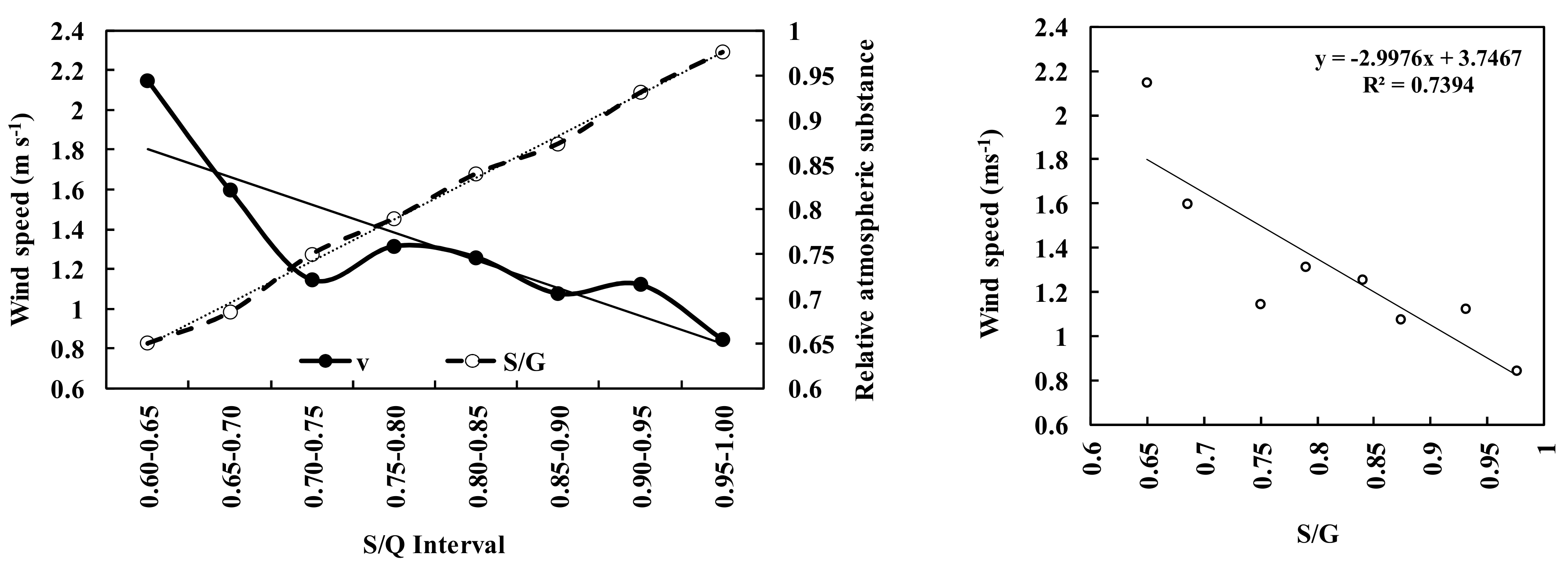
3.5. Correlations between Some Parameters and Related Mechanisms

To better understand interactions between different energy components and the atmospheric states (e.g., T, E, S/G) as well as atmospheric movement (e.g., wind speed), the correlations between any two monthly parameters and/or terms were analyzed. The monthly mean parameters include the absorbing term (e−kWm × cos(Z), AT) and the scattering term (ST) in Equation (3), air temperature (T), relative humidity, water vapor pressure, S/G, wind speed (v), and the square of the wind speed (v2). The results are shown in Table 8. To investigate the mechanisms clearly, a little cleaner atmospheric conditions, i.e., S/G < 0.75, were also considered in the analysis. G is an important driving factor in controlling the changes in the atmosphere (e.g., high correlations for T, then E, and S/G). ST is beneficial for the horizontal movement of the atmosphere than AT. These regularities were revealed evidently under S/G > 0.75 conditions.

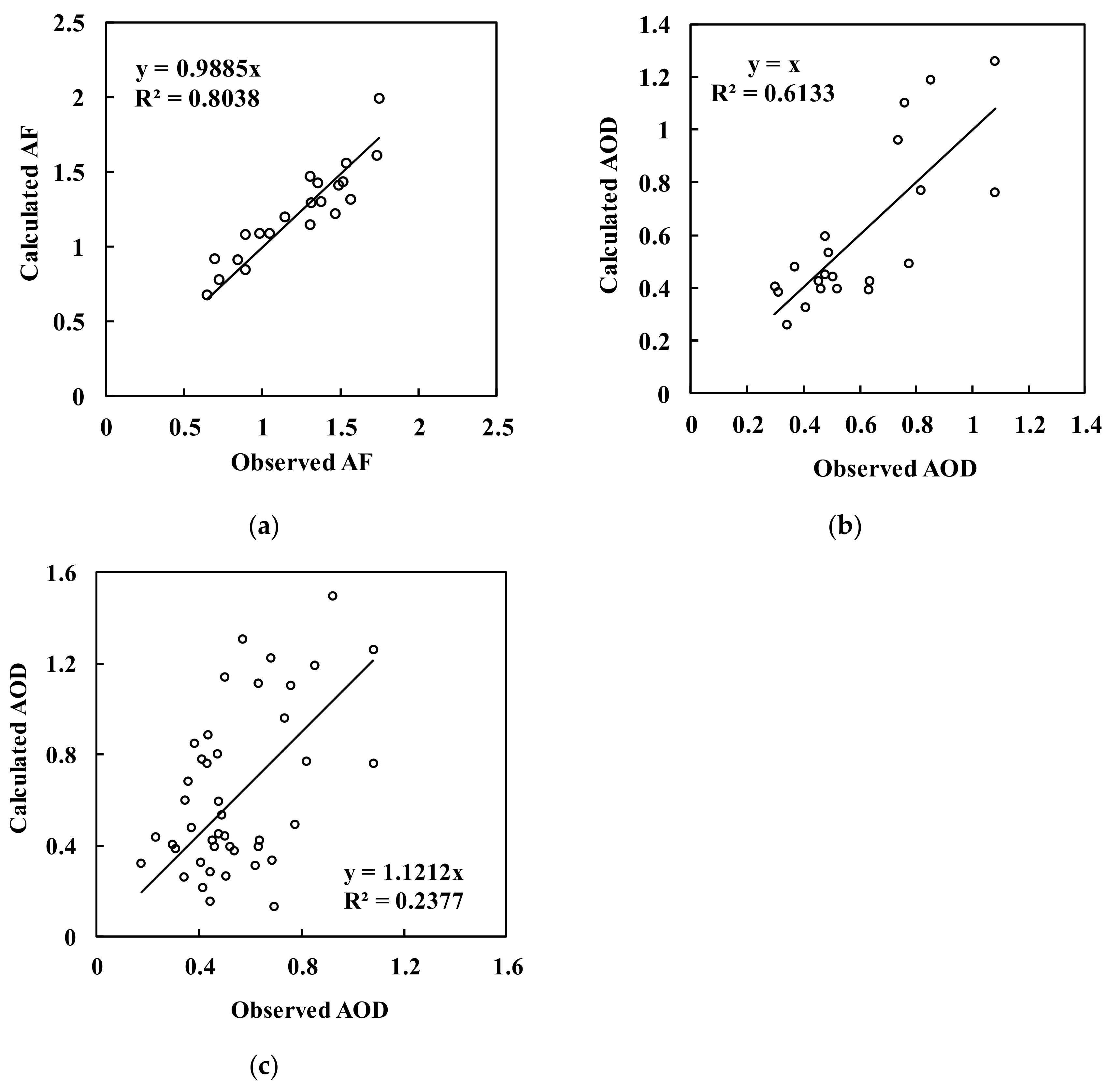
3.6. Estimation of Aerosol Optical Depth (AOD)

The aerosol optical depth (AOD) is an important parameter for understanding aerosols and their interactions with solar radiation, so it is desirable to obtain the AOD using global solar radiation. The monthly AOD from January 2013 until December 2016 was derived from the Moderate Resolution Imaging Spectroradiometer (MODIS) [38] aboard NASA (National Aeronautics and Space Administration)’s Terra satellite. Terra is flying in a near-polar sun-synchronous circular orbit since December 1999 and provides daily near-global coverage. The daily AOD Dark Target (DT) and Deep Blue (DB) merged L2 (10 × 10 km2 resolution) product (MOD04) was used to obtain AOD monthly aggregates. The DB algorithm [39] was originally developed for use over bright surfaces (e.g., over deserts, arid and semi-arid areas) where the DT algorithm [40] cannot be used reliably. DB was further developed for retrieving aerosol information over all land types [41]. An overview of the MODIS algorithm is presented in Levy et al. [42], and the most recent MODIS AOD data set is C6.1, which for China was validated by Sogacheva et al. [30]. For each location considered in the current manuscript, MODIS/Terra AOD C6.1 data were averaged over a radius of 50 km around the measurement site.
The results described in Section 3.3, i.e., the strong relation between the AF and E and S/G, suggested that in this relation, S/G could be replaced by the AOD as a proxy for scattering GLPs (n = 43, all monthly data, α = 0.001):
AF = B1 × E+ B2 × AOD+ B0
Similar to the calculation of S/G from the AF using Equation (5), the AOD was also calculated using Equation (6), independently (situation A).
To improve this relationship and decrease the estimation errors of the AF and/or the AOD, data with relative errors <50% were reanalyzed and a new equation was determined (n = 21, α = 0.001, situation B). Finally, monthly AOD values during January 2013–December 2016 were estimated using this new equation (n = 43, situation C). The main results for all three situations are summarized in Table 9. The mean relative errors for both the AF and the AOD are given for using the AOD to estimate the AF, or vice versa, using the AF to estimate the AOD. To better understand the basic characteristics of the atmosphere and solar irradiance, monthly mean values of the AOD from MODIS, global solar irradiance, and S/G under different situations are also shown in Table 9. The data in Table 9 show that both situations A and B are suitable for estimating the AOD, with situation B being somewhat better (e.g., δavgis smaller). This result shows that data quality is more important than data number in determining the internal regularity associated with atmospheric variables and processes, especially in developing an empirical model that captures and represents most regularities in the realistic atmosphere (e.g., n = 14 for developing the empirical model). As an example, scatter plots of the calculated vs. observed AF and AOD for situation B (Figure 8) show their good relationships.
These results show that it is feasible to obtain the AOD by using global radiation and meteorological parameters (i.e., AF and E). Compared to the calculation of S/G, the larger estimation error of the AOD (e.g., for situations A and C) was mainly caused by the limited number of AOD observations during each day (only one overpass per day) or month and the AOD retrieval error [42]. In summary, the relationships between the AF and S/G and between the AF and the AOD can be used to estimate S/G and the AOD.

4. Discussions

4.1. Empirical Model and Estimation of Global Solar Irradiance

Based on the analysis of representative radiation data measured in the natural laboratory, an empirical model of global solar radiation was developed. It describes the energy relationships between global solar irradiance and its absorbing and scattering components. The empirical model uses the ground observed water vapor amount (E) and the diffuse and global solar radiation (i.e., S/G) to express the absorbing and scattering substances, respectively, then, to estimate global radiation at the ground and at the TOA. If the observed S and G are not used in the empirical model (considering they are measured and need not be simulated), S/G can be replaced by other scattering factors (AF, AOD, etc.) based on the results in Section 3.3 and Section 3.6, and more studies are needed. However, the S/G factor can represent the scattering substances and their scattering roles objectively under all-sky conditions, and no assumptions are needed, i.e., it is a reliable parameter than the AF, the AOD, and others, and is suggested to be used so as to estimate global radiation and its components at the ground and at the TOA and their losses in the atmosphere accurately.
The performance of the empirical model, Equation (3), was evaluated by comparison with the solar constant, i.e., using the ratio of A1 + A2 + |A0| to the solar constant at the TOA. This ratio was 1.20 and 1.07 for S/G < 0.80 (n = 14) and S/G ≥ 0.80 (n = 29), respectively. When observational data with S/G larger than 0.70 was removed and reanalyzed, a similar empirical model was also determined and the above ratio decreased to 1.11 (n = 4, averaged S/G = 0.63). Generally, the simulation of G is reliable and improves in a cleaner atmosphere, and more data are helpful to investigate the model performance (e.g., n = 29).
Its usage is to calculate global radiation at the ground and at the TOA, as well as the loss in the atmosphere, associating with the absorbing and scattering GLPs, separately. Therefore, the interactions/mechanisms between absorbing and scattering global radiation and absorbing and scattering GLPs and meteorological variables (air temperature, water vapor, wind speed, humidity, etc.) can be investigated (e.g., Section 3.5) at present and in future studies. The albedos at the TOA and the ground can also be estimated using the empirical model (Section 4.5). If long-term observation data (>10 or 20 years) are available, an extensive study and understanding of the role of solar radiation in the atmospheric movement, regional climate, and climate change would be achieved. It should be emphasized that E and S/G represent the total absorbing and scattering GLPs in the entire atmospheric column.
The novelty of this study was to investigate the mechanisms between different energy components and the related parameters (temperature, wind speed, water vapor, S/G, etc.) and to study the albedos at the TOA and the ground for deeply understanding the solar radiation–atmosphere relations. The empirical model is an application of the empirical models previously developed for UV and visible wavelength bands under clear and all-sky conditions in North China [22,25].
Global solar radiation transfers in the atmosphere, where it is attenuated by two processes, absorption and scattering, which are independent of each other (Section 2.1 and Section 2.3). For GLPs, absorption of solar radiation influences the internal energy of the atmospheric molecules, which, in turn, affects air temperature and horizontal and vertical movements of the atmosphere (e.g., Table 8). In more detail, an increase in GLPs in the atmosphere leads to an increases in the local air temperature, together with absorbing energy (Table 8) at the level where these GLPs occur, and a decrease in global solar radiation at the surface and thus a decrease in the surface temperature. These two effects may result in a temperature inversion in the boundary layer. The more GLPs are produced through chemical and photochemical processes, the stronger and more stable is the temperature inversion. The mechanism of “absorption of solar radiation affects air temperature and the vertical movement of the atmosphere” has many potential applications, e.g., the increased air temperature and the decreased precipitation in Beijing and North China [43,44] and the decreasing wind speed in North China [45] during recent decades, with the increase in GLPs, including the AOD, HCHO (formaldehyde) vertical column density, AVOC (anthropogenic volatile organic compounds)and BVOC emissions, etc. [20,31], the direct radiative forcing [46], and large-scale circulations and the hydrological cycle, namely observed temperature and precipitation changes in China and India [47]. The weak convective activity and the accumulated GLPs (including air pollutants) result in a stable atmosphere, which remains so until a strong weather system arrives, which induces transport.
This point is further illustrated in Figure 9, where time series of the monthly mean wind speed and the monthly mean values of S/G observed at this site are presented for the period from June 2013 to December 2016. Figure 9 shows the contrasting behavior of S/G (increasing) and wind speed (decreasing) with overall fluctuations for the same month but with opposed signs. In addition, Figure 10 shows the monthly wind speed and the monthly atmospheric substance for the S/G interval at 0.05 ranging from 0.60 to 1.00. These observations support earlier observations referred to above: that smaller wind speed is associated with the accumulation of atmospheric substances and a larger S/G. Similarly, the negative correlations between S/G and v and between S/G and v2 also support the observations (Table 8). The much cleaner the atmosphere is (e.g., less S/G), the more evidently this mechanism is displayed.
The positive correlations between the absorbing energy (AT) and air temperature, between the scattering energy (ST) and v, and between the ST and v2, imply that absorbing and scattering energies used by GLPs may play different roles in the atmosphere and its movement.
Global solar radiation arriving at the surface and its losses in absorbing and scattering energy had clear seasonal and interannual variations in this subtropical site, as well as UV and visible radiation in North China [20,22]. Therefore, it is essential to thoroughly study its transfer and loss in the atmosphere, including the interactions and mechanisms between solar radiation energy and GLPs.
Global solar irradiance at the surface showed a decreasing tendency during 2013 to 2016, which is mainly caused by the increase in S/G and reflection at the TOA (Section 3.1), i.e., the change in atmospheric substances (e.g., emissions of all GLPs, all kinds of GLP products from VOC oxidation, clouds, etc.) gives rise to the variation in global solar radiation at the ground. It is observed that BVOC emissions increase during biomass burning and florescence and contribute to local cloud formation [36]. The cloudiness increased in JiangXi Province during 2001 to 2015 [48], corresponding to the increase in GLPs in the Qianyanzhou region to some extent. The increase in clouds and S/G indicates that the oxidation products of VOCs, mainly biogenic VOCs (BVOCs, e.g., isoprene, monoterpenes) at this subtropical plantation, contribute to the formation of cloud condensation nuclei (CCN) and regional clouds [33,35,49,50,51]. In other words, lots of GLPs consume (and/or transfer) UV and visible energy directly and/or indirectly through OH radials, including organic and inorganic compounds, such as O3, NO2, SO2, VOCs (especially more reactive and thousands of BVOCs), peroxides, acids, nitrates, organic aerosols (including SOA), and fine particles such as black carbon (BC) [20,31,32,52,53,54]. So, VOCs and their oxidation products, and the total GLPs are suggested to be considered in calculating and evaluating global solar radiation and its variation; though VOC concentrations are very low in the atmosphere, the accumulation of their total energy in direct absorption and indirect use should not be neglected [22,25]. Thus, it is also suggested to study long-term variations in total absorbing and scattering GLPs to explain regional dimming and brightening, apart from the factors that are commonly studied, such as aerosols, clouds, and wind speed [55,56].

4.2. Extinction Factor and the AOD

The relationships between the AF, E, and S/G and between the AF, E and the AOD, and the estimation of S/G and the AOD from the AF suggest the value of adding measurements of solar direct radiation at radiation sites in China and elsewhere in the world. These measurements will contribute to improving our understanding of radiation transfer and energy use in the atmosphere, as well as the mechanisms underlying regional climate and climate change.
The functions AF = f(E, S/G) and AF = f(E, AOD) are useful and better to estimate the AF with small relative errors than to estimate S/G or the AOD. The S/G derived from AF = f(E, S/G) is also suitable for the calculation of the attenuation of global solar radiation by scattering GLPs. The relative errors of S/G estimates were larger than those of AF estimates. For sites without direct solar radiation and AOD measurements, the equations AF = f (E, S/G) and AF = f (E, AOD) could be used as methods to estimate the historical S/G or AOD over China and other sites in the world for understanding aerosol variations in the long history of the past, when additional measurements of S/G or the AOD are carried out from now on. Studies of the radiation-derived AOD in China, e.g., Qiu and Xu et al. [57,58], show the potential of creating long time series, and the results compare favorably with independent reference AOD measurements from AERONET.

4.3. Relative Contributions of Absorbing and Scattering Terms

The contribution (RLA) of absorption (GLA) to the total loss of global solar irradiance GL was more important than that (RLS) of scattering (GLS) in the short-wavelength region, meaning that the absorbing substances in GLP phases attenuate more global solar radiation than the scattering substances at the subtropical Pinus forest, i.e., atmospheric GLPs exhibit more absorbing features. In other words, scattering GLPs play less important roles in attenuation. The annual ratios (RLA and RLS) are 35.3% and 67.7%, respectively, in the UV region (290–400 nm) and 4.7% and 95.3%, respectively, in the visible region (400–700 nm) in North China during 2004–2006. The UV radiation with higher frequency excites more GLP substances (e.g., O3, OH radials, H2O, NO2, SO2, VOCs, SOA) to take part in CPRs; thus, more energy is consumed in the UV band (35.30%) than in the visible band (4.70%) by GLPs [20,22]. Therefore, atmospheric GLPs show different characteristics on absorbing and scattering in UV, VIS, and G regions, where one, absorbing or scattering, is dominant and strongly depends on the wavelength and site type. So, the absorbing term and scattering term can describe each absorbing and scattering process very well in the above regions.
This implies that the total absorbing and scattering energy associated with all GLP constituents, no matter what sizes they have (e.g., molecules, H2O, particles), can be separated into and calculated by absorbing and scattering, respectively. The absorbing term expresses absorbing energy through different mechanisms in UV, VIS, and NIR regions (Section 4.4), whereas S/G contains the total scattering from all-size constituents (such as Raleigh and Mie scattering) in the whole atmosphere in different regions. In other words, when Equation (3) is applied in a specific wavelength region (e.g., UV, VIS, short wavelength), the realistic and independent roles of the two terms are determined by analyzing observational data. Taking another example, by application of Equation (3) to the UV region for the study of UV from January to December 1990 at Xianghe, 70 km from Beijing (China) [20], the monthly UV in the atmosphere under clear-sky conditions (N ≤2) was calculated for contributions from three factors (O3, water vapor pressure, and scattering) or two factors (water vapor and scattering). Here, the O3 term is introduced by e−k′1O3m, where k 1 [(3.30 ± 0.07) × 105 (Pa cm)−1] is the mean absorption coefficient of O3 in the wavelength range of 290.2–400.0 nm and O3 is the column-integrated concentration (Du). The monthly averages of O3 and absorbing terms were calculated using this new equation: their summations (O3 + absorbing terms) showed similar variations with the absorbing term calculated by Equation (3), and their relative bias was 6.5% (ranged from 1.7% to 17.0%). The new simulated monthly UV agreed with the measured UV, and its relative bias was 1.8% (0.1–2.7%). This equation was used to calculate the monthly UV in 1990 (N ≤ 2): when considering three terms (O3, absorbing term, and scattering term), the relative biases were 3.68% for the average and 12.39% for the maximum; when considering two terms (absorbing and scattering terms), the relative errors were 4.09% for the average and 10.68% for the maximum. The albedo values at the TOA were 16.9% and 16.8% for using three- and two-term equations, respectively. Then, monthly mean UV losses caused by O3 and absorbing terms using a three-term equation and by the absorbing term using a two-term equation were close, and their averages were 0.54 and 0.57 MJ m−2, respectively. Similarly, monthly mean UV losses caused by the scattering using three- and two-term equations were close: 0.26 and 0.23 MJ m−2, respectively. The annual averages of UV and tropospheric column NO2 showed similar variations at four sites in North China, and their correlation coefficient was 0.89, indicating that NO2 is a main UV absorber and giving an important hint that NO2 participates in OH and H2O photochemistry in the UV region [20]. The above results show that (1) the absorbing term can represent the role of O3, if O3 is not explicitly displayed in the equation, and (2) the absorbing term in the two-term equation can well express UV direct absorption and indirect use by all kinds of atmospheric GLPs, including the absorption of O3. This mechanism is further applied in the UV region, when other atmospheric constituents (e.g., NO2, VOCs) are not displayed in the equation, and also applied to the visible region based on the similar OH radical production and its photochemical role (Section 4.4) and the similar features in the UV and visible regions. (3) The scattering term can well describe the scattering roles of GLPs and the multiple reflections between GLPs and Earth’s surface [20].
The scattering factor S/G objectively describes the integrated scattering property of all kinds of substances in the atmosphere, including molecules, aerosols, clouds, rain, and multiple reflections between the surface and the atmosphere. However, cloudiness does not have the same effect as the S/G factor. S/G is a continuous and more accurate parameter than the cloudiness measured by observers, and hourly cloudiness is not available at most meteorological and radiation observation sites. Cloud type, structure, and other parameters (height, shape, position in the sky, etc.) influence the transfer of solar radiation. i.e., cloudiness is not good enough to quantitatively express the interactions/attenuations between the clouds and solar radiation.
In summary, solar energy in different regions plays different roles in energy usage, i.e., absorption and scattering. The total energy associated with all absorbing and scattering constituents is determined and estimated by two independent terms, respectively.

4.4. The Meaning of the Absorbing Term

The absorbing term represents the total absorption and/or use of global solar radiation by all GLPs in the short-wavelength region (including UV, VIS, and NIR). This is briefly explained as follows.
In the UV region, OH radicals are mainly produced by O3 photolysis (O3 + hv→O2 + O(1D), O(1D) + H2O→2OH) and the photolysis of HNO2, HNO3, and H2O2. The OH radical takes part in almost all CPRs. As reactors and catalysts in CPRs, water and water vapor play vital roles in UV consumption, e.g., reacting with SO2, NOx, VOCs, formic acid, aerosols, etc., and are recycled. Some molecules that do not consume UV directly react with OH, and their products may be oxidized in the atmosphere, and the second- and third-generation products may absorb UV radiation. Besides, several studies show that water vapor has absorption in the UV region [26,59]. So, UV energy is absorbed directly by some GLPs, e.g., NO2, SO2, O3, α-dicarbonyl compounds, ketone, benzaldehyde, NOCl, and light-absorbing aerosols, such as black carbon (BC) and organic carbon (OC), and/or consumed by other GLPs (without direct UV absorption) [20,32,53,60,61]. In more detail, wood smoke OC and BC, SOA produced from BVOC oxidation in the presence of NOx, and O3 absorb a comparable amount of UV and visible light [62,63,64,65].
In the visible region, a mechanism of OH radical production by an excited NO2* reaction with water molecules has been reported [24]. OH radical formation is also associated with photolysis of H2O and other GLPs, for example, CH3OOH. The large CH3OOH concentration in the troposphere makes this an important OH source [23]. During the formation of OH and HO2 radicals, there is also use and/or transfer of light energy to chemical energy, similar to the UV region [22]. More studies have reported the absorption, e.g., the pollution cloud absorbs solar radiation (0.53–3.30 μm) rather strongly compared with natural aerosols [66].
In the NIR region, H2O, CO2, CH4, and other GLPs absorb radiation directly and transfer and consume NIR energy directly and indirectly.
Under S/Q < 0.80 conditions, strong positive correlations between monthly UV, VIS, G, and NIR with water vapor pressure (n = 14) were found, and their correlation coefficients were 0.95, 0.93, 0.89, and 0.84, respectively (α = 0.001). The coefficient was the largest for UV, a little smaller for VIS, and the smallest for NIR, revealing an important mechanism that the production of OH radicals is highly related to water vapor—the higher the frequency of solar radiation, the stronger the frequency dependence.
More than 30,000 different BVOCs are thought to be released from vegetation [67]. New particle formation in boreal regions is related to monoterpene emissions and causes an estimated negative radiative forcing of about −0.2 to −0.9 Wm−2 [68]. Additionally, biogenic emissions have a significant negative effective radiative forcing over the southeastern United States [69]. It is emphasized that numerous BVOCs and their solar energy use in aerosol formation through chemical and photochemical reactions play key roles and should be considered in model studies. BVOC emissions increase with warming and might produce both negative and positive feedback on climate warming [70].
Why can all direct absorption and indirect use of solar radiation caused by atmospheric GLPs be expressed by the absorbing term? The formation of OH radicals is highly associated with the photolysis of O3, NO2, and H2O, and OH radicals participate in almost all CPRs (especially through VOCs in three phases) in the UV and visible regions. So, the column water vapor amount and its change can be a surrogate for all absorbing GLPs and their changes in CPRs. The examples of O3 and NO2 in Section 4.3 can be references. S/G is used as a surrogate for total scattering GLPs. Additionally, the absorbing term and scattering term had no strong correlation (R = 0.36 for S/G < 0.80 and R = 0.06 for S/G ≥0.80). Therefore, using the multiple fitting (Equation (3)), energy relationships/roles between G and absorbing and scattering terms were determined, and the contributions of absorbing and scattering due to GLPs to G were distributed to the absorbing term and scattering term, independently.
It is of note that photos transfer in the atmosphere through absorption or diffuse processes interacting with atmospheric GLPs, and the A1 and A2 values are their individual initial irradiance at the TOA without interactions with the GLPs in the atmosphere.
So, over the whole short-wave region, the total solar energy absorption and indirect use by all GLPs during their changes and conversions in gas particles is associated with H2O, OH radicals, and other GLPs (e.g., O3, NOx, SO2, VOCs) [20,22]. These complicated homogeneous and heterogeneous reactions can be simplified as H2O + OH + NOx + SO2 + VOCs + other GLPs + UV + VIS + NIR → new GLPs (O3, PM +...), where PM is particulate matter, including PM2.5, PM10, SOA, and secondary inorganic aerosols [31].
According to the above mechanisms, it is understandable that a strong correlation exists between G and the absorbing term, which represents the total direct absorption and indirect use by all sorts of GLPs in the short-wavelength region, i.e., half of the contribution from the UV and visible regions, as NIR is about half of G.
For instance, the 11-year average cloud radiative effect (all sky to clear sky) on atmospheric solar absorption is about +11 Wm−2, and the clouds enhance atmospheric solar absorption most distinctly at desert-like locations (little occurrence of clouds) [71]. It is concluded that atmospheric GLPs outside the clouds play important roles in solar absorption to some extent. Considering numerous VOCs and VOC-produced SOA, unknown mechanisms of SOA formation, and challenges in calculating their roles in radiative transfer and chemical models, it is an advantage for the empirical method that is developed based on analyzing recent observational data sets under real environmental conditions than pure models developed based on previous known parameters or coefficients, mechanisms that lagged with the real atmospheric conditions.
In view of the strong positive correlation between the absorbing term and temperature, it is suggested to control all kinds of or at least the main GLP emissions and productions (e.g., VOCs, NO2, SO2, O3, BC, SOA) with absorption in the UV, visible, and near-infrared regions, not just common greenhouse gases, such as CO2, CH4, and N2O, so as to reduce global warming. This is similar but complementary to the interaction between greenhouse gases and solar variability, as discussed by Solanki [2]. Newly produced GLPs through CPRs change the atmosphere and albedo at the TOA (Section 3.2). The combined effects of the contributing factors discussed above should be considered in future studies, including VOCs (key bridges in gas–liquid–particle conversions and associated solar energy use), new particle formation from the oxidation of BVOCs and AVOCs, and polluted clouds [72,73,74,75]. Hence, the emissions of AVOCs and artificial BVOCs (e.g., biomass burning, cutting of plants and grasses) should be controlled [31] because they influence the processes of radiative transfer and tropospheric photochemistry, air temperature, and albedos and therefore regional climate and climate change.

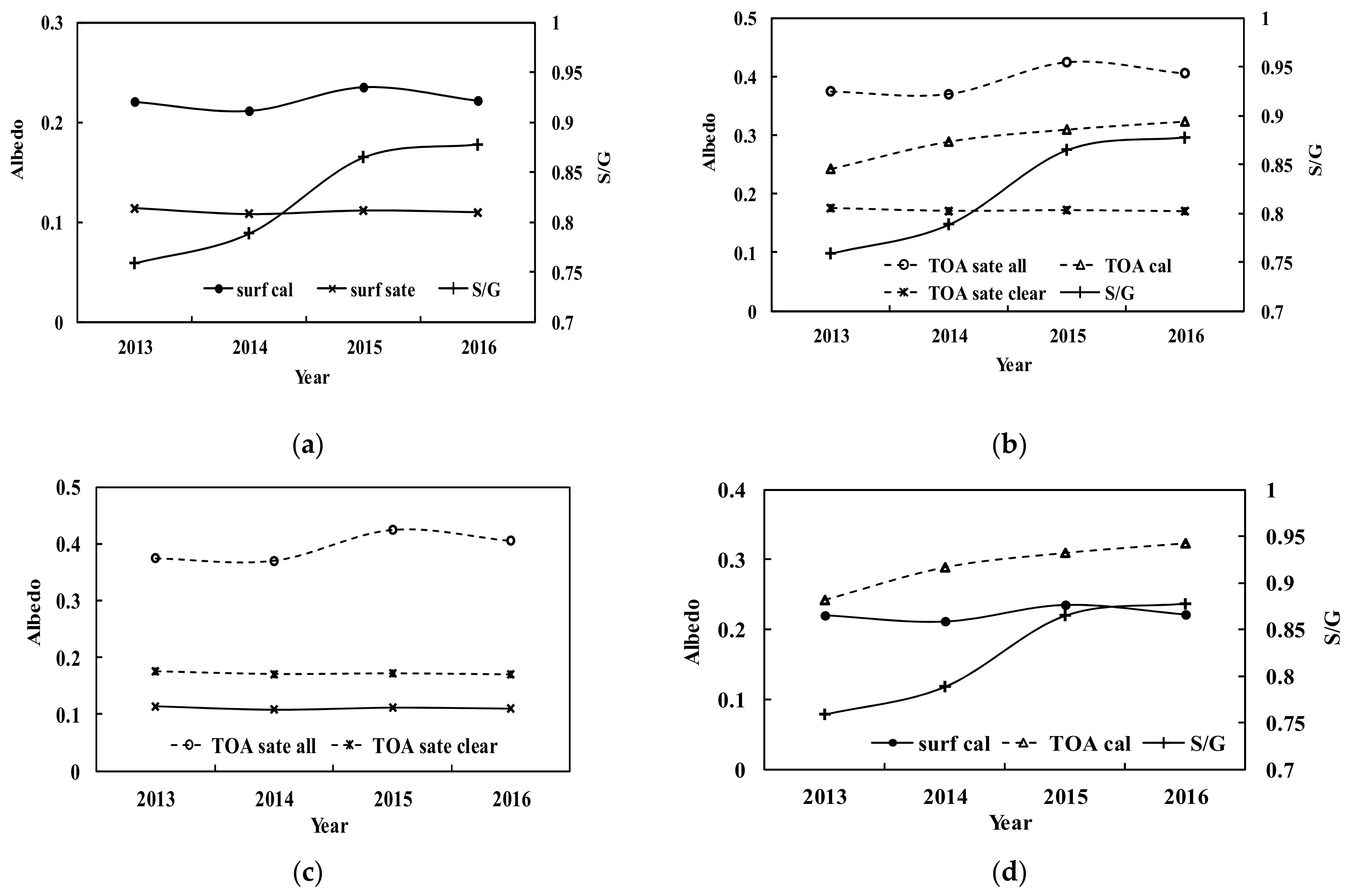
4.5. The Comparison of Albedo

Albedos at the TOA and at the surface are important factors influencing the energy budget, climate, and climate change [76,77,78]. Apart from using the radiative model and parameterization methods, another option is to obtain above two albedos using this empirical model and the ground observations. The absorbing and scattering processes are separated to two terms, giving a further application of the empirical model.
The Clouds and the Earth’s Radiant Energy System (CERES) Energy Balanced and Filled (EBAF) Edition 4.1 [79,80] provides the monthly shortwave flux and incoming solar flux on the TOA for all-sky, clear (for cloud free) sky and clear sky with a resolution of 1° × 1° (https://ceres.larc.nasa.gov/products.php?product=EBAF-Product, accessed on 13 March 2021). The albedos at the TOA from 2013 to 2016 were 24.23%, 28.29%, 30.95% and 32.33%, and calculated by the upward solar irradiance divided by downward solar irradiance using the coefficients from solar radiation empirical model, Equation (3) (Table 1):
albedo at the TOA = A0/(A1+A2)
Similarly, the albedo at the surface was calculated:
albedo at the surface = A0 × Atte/(A1e−kWm × cos(Z) + A2e−S/G)
Atte = 1 − e−S/G
The extinction rate (Atte) of the scattering term was used to estimate the attenuation of the reflection A0 at the surface. Generally, under all sky conditions, the satellite-retrieved albedo at the TOA from the monthly satellite-retrieved radiances and albedos at the TOA and at the surface calculated using Equations (7) and (8) showed similar year to year variations and an increase during 2013 to 2016 (Figure 11). The satellite-retrieved albedos (0.39) were larger than those calculated at the TOA (0.29), with relative bias of 26.07% and absolute error of 0.10 for the 4-year average. Under all skies, the calculated albedos at the TOA were larger than those at the surface, corresponding to the satellite-retrieved albedos, due to more reflected solar radiation arriving at the TOA. During four years, the satellite retrieved and the calculated albedos at the TOA increased by 4.09% and 11.73% per year, respectively, associating with the increase of S/G by 6.08% per year. Similarly, the albedos at the TOA under clear sky conditions (Figure 11a) were compared, and the satellite albedo was 0.17, a little less than the calculated value of 0.21, with a relative bias of 23.02% and an absolute error of 0.04 for the 4-year average. This is smaller than the error of the albedo retrieved by MODIS data in the shortwave band of 85.9% [81]. It should be mentioned that the albedo for cloudy conditions (N ≤ 0.80 and S/G < 0.80) is larger than in clear sky conditions. So, a better agreement was obtained for clear skies than all skies. The differences in calculated and satellite obtained albedos are due to the match-up in time and space, different wavebands (e.g., 0.27–3.20 μm vs 0.3–5.0 μm for the ground and satellite sensors, respectively), as well as the observational errors of solar radiation at the ground and on the satellite. The increase of atmospheric GLPs (S/G) caused the increase of albedo at the TOA under all skies (Figure 11a).
The satellite measured albedos were smaller than those calculated at the surface by about 50.03% (absolute difference = 0.11). Both the satellite measured and the calculated albedos at the surface decreased at 0.80% per year during this 4-year study. It may be caused by the increase of atmospheric GLPs (e.g., S/G) (Figure 11b). During four years, the satellite measured albedo at the TOA was larger than the surface albedo by 0.28, and the calculated albedo at the TOA was large than the surface albedo by 0.07. The large differences for satellite retrieved and calculated albedo were associated with high S/G (Figure 11c,d).
The albedo can be calculated using the empirical model (Equations (7) and (8)), and radiative transfer models [78] that require more atmospheric inputs, including aerosol, cloud and water properties [82], but not using the current empirical models mentioned in the introduction, i.e., progress has been made for the empirical model.
The decrease of global solar radiation at the ground is associated with energy losses: (1) absorption and scattering caused by GLP changes, including aerosols, clouds, gases, water vapor, and (2) the increase of reflection at the TOA. All these factors contribute the solar dimming and/or brightening and are suggested to be considered together, not only the individual aerosols, air pollutants [83,84] and clouds.
The yearly mean global irradiance retrieved from satellite data and that measured at the surface were in good agreement. The ratio between the satellite-retrieved and surface-measured values ranged from 0.91 to 1.09, with an average of 0.97. During four years, both the albedos at the TOA and the surface showed similar characteristics, e.g., higher at the TOA and lower at the surface, and varied in a similar way. In addition, with the increase of S/G, the albedo at the TOA increased, and the albedo at the surface decreased (Figure 11). Thus, the empirical model provided reasonable estimations of albedo at the TOA and the surface.
In short, the integrated studies on surface and satellite measured solar radiation, its extinction in the atmosphere, albedos at the surface and the TOA, as well as the interactions between all kinds of GLPs and solar radiation are suggested for a thorough understanding of radiative transfer in the whole atmosphere, regional dimming or brightening, energy balance [85], and climate and climate change. This kind of empirical model is suggested to be developed and used to study solar radiation and associated issues at other sites.

4.6. Seasonal Losses of Global Solar Irradiance Due to GLP Extinction

In summer and autumn (Section 3.1), RLS was much larger for low and high GLPs (S/G < 0.80 and S/G ≥ 0.80) than other seasons, implying the strong aerosol scattering contributed by SOA that produced form the oxidation of BVOCs. As this subtropical Pinus forest is a large BVOC emission source, and their emissions are higher in summer and autumn [36].
Seasonal RLA was larger by 12.21–16.20% in high GLPs (S/G ≥ 0.80) than that in low GLPs (S/G < 0.80) for all seasons (Table 2 and Table 3), the corresponding annual RLA was 90.98% and 76.77%, this was mainly due to numerous absorbing GLPs accumulated in high GLP loadings. These absorbing GLPs include BVOCs, NOx, SO2, O3, OC, etc. The NO2 and NOx concentrations were 3.12 and 5.15 ppb in September in 2014, O3 concentration ranged from 49.8 to 110.9 ppb in July–November 2014 [36]. Similarly, 35–47% of the light absorption contributed by biogenic particles during the wet-to-dry/wet season in the Amazon Basin is reported by Guyon et al. [86].
In four seasons, both GLS and RLS were larger by a factor of 2–4 at low GLP loads than that in high GLP loads, e.g., the averaged GLS was 135.50 (117.21–144.62) Wm−2 for S/G < 0.80 and 45.06 (37.02–50.06) Wm−2 for S/G ≥ 0.80, revealing that the relative small sized aerosols contribute much larger scattering at low aerosol loadings than that in high aerosol loadings. It should be emphasized that the small sized aerosols are produced from BVOC photochemical reactions under relatively low S/G and high light levels. With more and more GLP accumulations in the atmosphere in S/G ≥ 0.80 from S/G < 0.80, the contribution of light extinction dropped to 9.02% (6.59–11.18%) for GLP scattering and enhanced to 90.98% (88.82–93.41%) for GLP absorption, together with the large drop of loss in scattering and enhancement in absorbing to 468.42 Wm−2 from 455.22 Wm−2, indicating that the increases of GLP sizes by moisture-absorbing, aerosol coagulation processes with the increase of relative humidity to 78.47% (72.10–80.99%) form 70.23%, so, the extinction of global solar radiation was dominated by the absorbing rather than the scattering. More attention should be paid to GLPs, especially BVOCs and biogenic aerosols, as well as their radiation extinction. BVOC concentrations are much lower than NOx, SO2, O3, but, they take part in CPRs, absorb and/or utilize solar radiation that varies with atmospheric conditions. Therefore, the absorption and scattering caused by GLPs thorough OH, BVOCs and biological aerosols should be taken into account in radiative transfer and chemical models [86] at the forests and other regions, which is based on the observations, the large contributions of SOA in organic aerosols (~70%) in North China [87,88] and the increase of land greening in China recently and in the future [89]. In general, empirical models show lower performance for cloudy and overcast skies than clear skies [9,10,11,12,13,14,15,16,17,18,19,90], indicating that the high GLP loads (e.g., aerosols, clouds) and types are main reasons [90], the GLP amount and composition changes result in the changes in absorbing and scattering features, and their losses in the atmosphere (Section 3.1, Section 3.2, Section 3.3, Section 3.4, Section 3.5 and Section 3.6). It is still a challenge to improve the simulation of solar radiation in cloudy and overcast skies, i.e., accurate representation of the aerosol and a cloud property is needed [90].
The strong negative correlations were −0.95, −0.85 and −0.96 between the seasonal losses in absorbing, scattering and total global radiation with wind speed for S/G < 0.80, respectively, revealing a mechanism that the losses of solar radiation in the atmosphere weaken the atmospheric movement horizontally.

5. Conclusions

Based on the analysis of solar radiation and meteorological variables measured in a subtropical forest in China during 2013 to 2016, a new empirical model of global solar irradiance was developed and applied to calculate global solar radiation at the ground and its loss in the atmosphere due to absorption and scattering. The model can well separate the individual contributions from absorption and scattering, and the results were used to investigate the mechanisms associated with these two types of energy and atmospheric parameters. The calculated and observed global solar irradiances were in good agreement under different atmospheric conditions. The albedos at the TOA during 2013 to 2016 were 21.19% and 25.48%, respectively, for S/G < 0.80 and S/G ≥ 0.80, similar to satellite-derived albedos. Observed and calculated global solar irradiances decreased by −5.55% per year and −3.93% per year, respectively. Equations of the extinction factor (AF) with E and S/G and of the AF with E and the AOD can be used to estimate S/G or the AOD. The AF obtained using only global solar radiation is a useful factor. An empirical model of global solar radiation using the AF is suggested when S/G is not available. The losses of global solar energy caused by absorbing and scattering GLPs show clear seasonal and interannual variations.
There is an evident frequency dependency in correlations between UV, VIS, and NIR with E, revealing a mechanism that atmospheric substances have strong direct absorption and indirect use in UV than in VIS, and G through OH radicals. There was large extinction due to GLP scattering in summer and autumn, which is mainly attributed to the SOA that are produced from BVOC oxidation.
The negative correlations between S/G and v and between S/G and v2 indicate that the accumulation of atmospheric GLPs results in low wind speed and stagnant weather conditions, much loss of global solar radiation by absorbing, and stronger absorbing features of the atmosphere, especially in very high GLP loadings (compare S/G ≥ 0.80 to S/G < 0.80). The losses of solar radiation in absorbing and scattering weaken the horizontal motion of air.
The losses of global solar irradiance caused by total absorbing and scattering substances had evident seasonal and interannual variations during 2013–2016. The loss of global solar irradiance in the atmosphere was dominated by absorbing. In addition, the reflection at the TOA was another loss of global solar radiation. Sensitivity analysis indicates that global solar irradiance is more sensitive to changes in scattering (quantified by S/G) than to changes in absorption (quantified by water vapor pressure), and the responses of global solar irradiance to absorbing and scattering factors were negative and nonlinear. To reduce regional and global warming, it is suggested to control all kinds of GLP emissions and production of secondary air pollutants, not only limited known greenhouse gases. The absorbing and scattering irradiance due to total absorbing and scattering GLPs were calculated at the TOA, in the atmosphere and at the surface, and it is helpful to thoroughly understand the radiative transfer, energy budget, energy–GLP interactions, and energy–atmosphere movements.

Author Contributions

Methodology, investigation, and writing, J.B.; satellite albedo, X.Z. All authors have read and agreed to the published version of the manuscript.

Funding

This research was supported by the Strategic Priority Research Program of the Chinese Academy of Sciences (grant no. XDA19070202), the National Key R&D Program of China (grant no. 2016YFB 0500602), the National Natural Science Foundation of China (grant nos. 41275137 and 41675032), Dragon 4 and 5 projects (ID 32771 and 59013), and the European Union (EU) 7 framework programme MarcoPolo (grant no. 606953).

Institutional Review Board Statement

Not applicable.

Data Availability Statement

Not applicable.

Acknowledgments

The Terra/MODIS monthly AOD was acquired from the Level-1 and Atmosphere Archive & Distribution System (LAADS) Distributed Active Archive Center (DAAC), located in the Goddard Space Flight Center in Greenbelt, Maryland (https://ladsweb.nascom.nasa.gov/, accessed on 13 March 2021). Satellite albedos can be accessed via the website https://ceres.larc.nasa.gov/products.php?product=EBAF-Product (accessed on 13 March 2021) for this research measured at Qianyanzhou Station are published on a Big Earth Data Platform for Three Poles, http://poles.tpdc.ac.cn/zh-hans/ (accessed on 13 March 2021). The authors thank Gerrit de Leeuw and Larisa Sogacheva from the Finnish Meteorological Institute for constructive comments and providing satellite AOD data. The authors thank H.M. Wang, F.T. Yang, Q.K. Li, G.Z. Liu, L. Huang, Y.G. Wang, S.Y. Yin, J.D. Zou, J.Z. Zhang, Y.F. Huang, and G.L. Zhu at Taihe County, Jiangxi Province, and X.W. Wan and Y.M. Wu from the Institute of Atmospheric Physics, Chinese Academy of Sciences (CAS). The authors give special thanks to anonymous reviewers for their beneficial comments. The authors also thank the Qianyanzhou Experimental Station, CAS, for providing meteorological and solar radiation data from January to May 2013.

Conflicts of Interest

The authors declare no conflict of interest.

References

  1. Madronich, S.; Flocke, S. The Role of Solar Radiation in Atmospheric Chemistry. In Environmental Photochemistry, Vol. 2/2L of the Handbook of Environmental Chemistry; Boule, P., Ed.; Springer: Berlin/Heidelberg, Germany, 1999; pp. 1–26. [Google Scholar]
  2. Solanki, S.K. Solar variability and climate change is there a link. Astron. Geophys. 2002, 43, 5.9–5.13. [Google Scholar] [CrossRef] [Green Version]
  3. Elminir, H.K. Relative influence of weather conditions and air pollutants on solar radiation—Part 2: Modification of solar radiation over urban and rural sites. Meteorol. Atmos. Phys. 2007, 96, 257–264. [Google Scholar] [CrossRef]
  4. Trenberth, K.E.; Fasullo, J.T.; Kiehl, J. Earth’s global energy budget. Bull. Am. Meteorol. Soc. 2009, 90, 311–323. [Google Scholar] [CrossRef]
  5. Lean, J.; Rind, D. Climate forcing by changing solar radiation. J. Clim. 2010, 11, 3069–3094. [Google Scholar] [CrossRef]
  6. Andreae, M.O.; Ramanathan, V. Climate’s Dark Forcings. Sciences 2013, 340, 280–281. [Google Scholar] [CrossRef]
  7. Rosenfeld, D.; Sherwood, S.; Wood, R.; Donner, L. Climate Effects of Aerosol-Cloud Interactions. Sciences 2014, 343, 379–380. [Google Scholar] [CrossRef]
  8. Calabrò, E.; Magazù, S. Correlation between Increases of the Annual Global Solar Radiation and the Ground Albedo Solar Radiation due to Desertification—A Possible Factor Contributing to Climatic Change. Climate 2016, 4, 64. [Google Scholar] [CrossRef] [Green Version]
  9. Glower, J.; McGulloch, J.S.G. The empirical relation between solar radiation and hours of sunshine. Q. J. R. Met. Soc. 1958, 84, 172–175. [Google Scholar]
  10. Atwater, M.A.; Ball, J.T. A numerical solar radiation model based on standard meteorological observations. Sol. Energy 1978, 21, 163–170, Erratum in Sol. Energy 1978, 123, 275. [Google Scholar] [CrossRef]
  11. Bird, R.E. A simple solar spectral model for direct-normal and diffuse horizontal irradiance. Sol. Energy 1984, 32, 461–471. [Google Scholar] [CrossRef]
  12. Gueymard, C.A. Critical analysis and performance assessment of clear sky solar irradiance models using theoretical and measured data. Sol. Energy 1993, 51, 121–138. [Google Scholar] [CrossRef]
  13. Gueymard, C.A. Clear-Sky Radiation Models and Aerosol Effects. Sol. Resour. Mapp. 2019, 137–182. [Google Scholar] [CrossRef]
  14. Myers, D.R. Solar radiation modeling and measurements for renewable energy applications data and model quality. Energy 2005, 30, 1517–1531. [Google Scholar] [CrossRef]
  15. Badescu, V.; Gueymard, C.A.; Cheval, S.; Oprea, C.; Baciu, M.; Dumitrescu, A.; Iacobescu, F.; Milos, I.; Rada, C. Accuracy analysis for fifty-four clear-sky solar radiation models using routine hourly global irradiance measurements in Romania. Renew. Energy 2013, 55, 85–103. [Google Scholar] [CrossRef]
  16. Besharat, F.; Dehghan, A.A.; Faghih, A. Empirical models for estimating global solar radiation: A review and case study. Renew. Sustain. Energy Rev. 2013, 21, 798–821. [Google Scholar] [CrossRef]
  17. Bayrakc, H.C.; Demircan, C.; Keceba, A. The development of empirical models for estimating global solar radiation on horizontal surface: A case study. Renew. Sustain. Energy Rev. 2018, 81, 2771–2782. [Google Scholar] [CrossRef]
  18. Antonanzas-Torres, F.; Urraca, R.; Polo, J.; Perpinan-Lamigueiro, O.; Escobar, R. Clear sky solar irradiance models: A review of seventy models. Renew. Sustain. Energy Rev. 2019, 107, 374–387. [Google Scholar] [CrossRef]
  19. Kosmopoulos, P.G.; Kazadzis, S.; Lagouvardos, K.; Kotroni, V.; Bais, A. Solar energy prediction and verification using operational model forecasts and ground-based solar measurements. Energy 2015, 93, 1918–1930. [Google Scholar] [CrossRef]
  20. Bai, J.H. UV extinction in the atmosphere and its spatial variation in North China. Atmos. Environ. 2017, 154, 318–330. [Google Scholar] [CrossRef]
  21. Bilbao, J.; Mateos, D.; De Miguel, A. Analysis and cloudiness influence on UV total irradiation. J. Climatol. 2011, 31, 451–460. [Google Scholar]
  22. Bai, J.H. Photosynthetically active radiation loss in the atmosphere in North China. Atmos. Pollut. Res. 2013, 4, 411–419. [Google Scholar] [CrossRef] [Green Version]
  23. Matthews, J.; Sinha, A.; Francisco, J.S. The importance of weak absorption features in promoting tropospheric radical production. Proc. Natl. Acad. Sci. USA 2005, 102, 7449–7452. [Google Scholar] [CrossRef] [PubMed] [Green Version]
  24. Li, S.P.; Matthews, J.; Sinha, A. Atmospheric hydroxyl radical production from electronically excited NO2 and H2O. Science 2008, 319, 1657–1660. [Google Scholar] [CrossRef]
  25. Bai, J.H. Analysis of ultraviolet radiation in clear skies in Beijing and its affecting factors. Atmos. Environ. 2011, 45, 6930–6937. [Google Scholar] [CrossRef]
  26. Du, J.; Huang, L.; Min, Q.; Zhu, L. The Influence of Water Vapor Absorption in the 290–350 nm Region on Solar Radiance: Laboratory Studies and Model Simulation. Geophys. Res. Lett. 2013, 40, 1–5. [Google Scholar] [CrossRef]
  27. Wilson, E.M.; Wenger, J.C.; Venables, D.S. Upper limits for absorption by water vapor in the near-UV. J. Quant. Spectrosc. Radiat. Transf. 2016, 170, 194–199. [Google Scholar] [CrossRef]
  28. Kondratyev, K.Y.A. Solar Energy; Science Press: Beijing, China, 1962; pp. 123–132. [Google Scholar]
  29. Yang, S.; Wang, X.L.; Wild, M. Causes of Dimming and Brightening in China Inferred from Homogenized Daily Clear-Sky and All-Sky in situ Surface Solar Radiation Records (1958–2016). J. Clim. 2019, 32, 5901–5913. [Google Scholar] [CrossRef]
  30. Sogacheva, L.; de Leeuw, G.; Rodriguez, E.; Kolmonen, P.; Georgoulias, A.K.; Alexandri, G.; Kourtidis, K.; Proestakis, E.; Marinou, E.; Amiridis, V.; et al. Spatial and seasonal variations of aerosols over China from two decades of multi-satellite observations—Part 1: ATSR (1995–2011) and MODIS C6.1 (2000–2017). Atmos. Chem. Phys. 2018, 18, 11389–11407. [Google Scholar] [CrossRef] [Green Version]
  31. Bai, J.; de Leeuw, G.; De Smedt, I.; Theys, N.; Van Roozendael, M.; Sogacheva, L.; Chai, W. Variations and photochemical transformations of atmospheric constituents in North China. Atmos. Environ. 2018, 189, 213–226. [Google Scholar] [CrossRef]
  32. Jacobson, M. Isolating nitrated and aromatic aerosols and nitrated aromatic gases as sources of ultraviolet light absorption. J. Geophys. Res. 1999, 104, 3527–3542. [Google Scholar] [CrossRef]
  33. Claeys, M.; Graham, B.; Vas, G.; Wang, W.; Vermeylen, R.; Pashynska, V.; Cafmeyer, J.; Guyon, P.; Andreae, M.O.; Artaxo, P.; et al. Formation of secondary organic aerosols through photooxidation of isoprene. Science 2004, 303, 1173–1176. [Google Scholar] [CrossRef] [PubMed] [Green Version]
  34. Jonsson, Å.M.; Hallquist, M.; Ljungström, E. Influence of OH Scavenger on the Water Effect on Secondary Organic Aerosol Formation from Ozonolysis of Limonene, Δ3-Carene, and α-Pinene. Environ. Sci. Technol. 2008, 42, 5938–5944. [Google Scholar] [CrossRef]
  35. Carlton, A.G.; Wiedinmyer, C.; Kroll, J.H. A review of secondary organic aerosol (SOA) formation from isoprene. Atmos. Chem. Phys. 2009, 9, 4987–5005. [Google Scholar] [CrossRef] [Green Version]
  36. Bai, J.H.; Guenther, A.; Turnipseed, A.; Duhl, T.; Greenberg, J. Seasonal and interannual variations in whole-ecosystem BVOC emissions from a subtropical plantation in China. Atmos. Environ. 2017, 161, 176–190. [Google Scholar] [CrossRef]
  37. Hansel, A.K.; Ehrenhauser, F.S.; Richards-Henderson, N.K.; Anastasio, C.; Valsaraj, K.T. Aqueous-phase oxidation of green leaf volatiles by hydroxyl radical as a source of SOA: Product identification from methyl jasmonate and methyl salicylate oxidation. Atmos. Environ. 2015, 102, 43–51. [Google Scholar] [CrossRef]
  38. Salomonson, V.V.; Barnes, W.L.; Maymon, P.W.; Montgomery, P.W.; Ostrow, H. MODIS: Advanced facility instrument for studies of the Earth as a system. IEEE Trans. Geosci. Remote Sens. 1989, 27, 145–153. [Google Scholar] [CrossRef]
  39. Hsu, N.C.; Tsay, S.C.; King, M.D.; Herman, J.R. Aerosol properties over bright-reflecting source regions. IEEE Trans. Geosci. Remote Sens. 2004, 42, 557–569. [Google Scholar] [CrossRef]
  40. Remer, L.A.; Kaufman, Y.J.; Tanré, D.; Mattoo, S.; Chu, D.A.; Martins, J.V.; Li, R.R.; Ichoku, C.; Levy, R.C.; Kleidman, R.G.; et al. The MODIS Aerosol Algorithm, Products, and Validation. J. Atmos. Sci. 2005, 62, 947–973. [Google Scholar] [CrossRef] [Green Version]
  41. Sayer, A.M.; Munchak, L.A.; Hsu, N.C.; Levy, R.C.; Bettenhausen, C.; Jeong, M.J. MODIS Collection 6 aerosol products: Comparison between Aqua’s e-Deep Blue, Dark Target, and “merged” data sets, and usage recommendations. J. Geophys. Res. Atmos. 2014, 119, 13965–13989. [Google Scholar] [CrossRef]
  42. Levy, R.C.; Mattoo, S.; Munchak, L.A.; Remer, L.A.; Sayer, A.M.; Patadia, F.; Hsu, N.C. The Collection 6 MODIS aerosol products over land and ocean. Atmos. Meas. Tech. 2013, 6, 2989–3034. [Google Scholar] [CrossRef] [Green Version]
  43. Yang, H. Analysis on climate change feature of Beijing during 1951 to 2006. Beijing Water 2013, 3, 36–40. [Google Scholar]
  44. Zhang, Y.X.; Song, M.; Yang, Y.J. The change characteristic of temperature and precipitation in the North China during 1956 and 2011. J. Anhui Agric. Sci. 2013, 4, 41726–41728. [Google Scholar]
  45. Rong, Y.Q.; Liang, J.Y. Analysis of variation of wind speed over north China. Sci. Meteorol. Sin. 2015, 28, 655–658. [Google Scholar]
  46. Jacobson, M.Z. Strong radiative heating due to the mixing state of black carbon in atmospheric aerosols. Nature 2001, 409, 695–697. [Google Scholar] [CrossRef]
  47. Menon, S.; Hansen, J.; Nazarenko, L.; Luo, Y.F. Climate effects of black carbon aerosols in China and India. Science 2002, 297, 2250–2253. [Google Scholar] [CrossRef] [Green Version]
  48. Ma, Q.R.; You, Q.L.; Cai, M.; Zhou, Y.Q.; Liu, J.J. The cloud variation over China in recent 15 years based on CERES satellite data. J. Arid Meteorol. 2018, 36, 911–920. [Google Scholar]
  49. Ehn, M.; Thornton, J.A.; Kleist, E.; Sipilä, M.; Junninen, H.; Pullinen, I.; Springer, M.; Rubach, F.; Tillmann, R.; Lee, B.; et al. A large source of low-volatility secondary organic aerosol. Nature 2014, 506, 476–479. [Google Scholar] [CrossRef] [PubMed]
  50. McVay, R.C.; Zhang, X.; Aumont, B.; Valorso, R.; Camredon, M.; La, Y.Y.S.; Wennberg, P.O.; Seinfeld, J.H. SOA formation from the photooxidation of α-pinene: Systematic exploration of the simulation of chamber data. Atmos. Chem. Phys. 2016, 16, 2785–2802. [Google Scholar] [CrossRef] [Green Version]
  51. Dunne, E.M.; Gordon, H.; Kürten, A.; Almeida, J.; Duplissy, J.; Williamson, C.; Ortega, I.K.; Pringle, K.J.; Adamov, A.; Baltensperger, U.; et al. Global atmospheric particle formation from CERN CLOUD. Science 2016, 354, 1119–1124. [Google Scholar] [CrossRef] [PubMed] [Green Version]
  52. Atkinson, R. Atmospheric chemistry of VOCs and NOx. Atmos. Environ. 2000, 34, 2063–2101. [Google Scholar] [CrossRef]
  53. Kirchstetter, T.W.; Novakov, T.; Hobbs, P.V. Evidence that the spectral dependence of light absorption by aerosols is affected by organic carbon. J. Geophys. Res. 2004, 109, D21208. [Google Scholar] [CrossRef] [Green Version]
  54. Hoffer, A.; Gelencs’er, A.; Guyon, P.; Kiss, G.; Schmidt, O.; Frank, G.P.; Artaxo, P.; Andreae, M.O. Optical properties of humic-like substances (HULIS) in biomass burning aerosols. Atmos. Chem. Phys. 2006, 6, 3563–3570. [Google Scholar] [CrossRef] [Green Version]
  55. Wild, M.; Gilgen, H.; Roesch, A.; Ohmura, A.; Long, C.; Dutton, E.; Forgan, B.; Kallis, A.; Russak, V.; Tsvetkov, A. From dimming to brightening: Decadal changes in solar radiation at the Earth’s surface. Science 2005, 308, 847–850. [Google Scholar] [CrossRef] [Green Version]
  56. Wang, Y.W.; Yang, Y.H. China’s dimming and brightening: Evidence, causes and hydrological implications. Ann. Geophys. 2014, 32, 1–15. [Google Scholar] [CrossRef] [Green Version]
  57. Qiu, J. A Method to Determine Atmospheric Aerosol Optical Depth Using Total Direct Solar Radiation. J. Atmos. Sci. 1998, 55, 744–757. [Google Scholar] [CrossRef]
  58. Xu, X.; Qiu, J.; Xia, X.; Sun, L.; Min, M. Characteristics of atmospheric aerosol optical depth variation in China during 1993–2012. Atmos. Environ. 2015, 119, 82–94. [Google Scholar] [CrossRef]
  59. Lampel, J.; Pöhler, D.; Polyansky, O.; Kyuberis, A.A.; Zobov, N.F.; Tennyson, J.; Lodi, L.; Frieß, U.; Wang, Y.; Beirle, S.; et al. Detection of water vapour absorption around 363 nm in measured atmospheric absorption spectra and its effect on DOAS evaluations. Atmos. Chem. Phys. 2017, 17, 1271–1295. [Google Scholar] [CrossRef] [Green Version]
  60. Meller, R.; Moortgat, G.K. Temperature dependence of the absorption cross sections of formaldehyde between 223 and 323 K. J. Geophys. Res. 2000, 105, 7089–7101. [Google Scholar] [CrossRef]
  61. Horowitz, A.; Meller, R.; Moortgat, G.K. The UV-VIS absorption cross sections of the α- dicarbonyl compounds: Pyruvic acid, biacetyl and glyoxal. J. Photochem. Photobiol. A Chem. 2001, 146, 19–27. [Google Scholar] [CrossRef]
  62. Adamopoulos, A.D.; Kambezidis, H.D.; Zevgolis, D. Total atmospheric transmittance in the ultraviolet and visible spectra in Athens, Greece. Pure Appl. Geophys. 2005, 162, 409–431. [Google Scholar] [CrossRef]
  63. Kirchstetter, T.W.; Thatcher, T.L. Contribution of organic carbon to wood smoke particulate matter absorption of solar radiation. Atmos. Chem. Phys. 2012, 12, 6067–6072. [Google Scholar] [CrossRef] [Green Version]
  64. Desyaterik, Y.; Sun, Y.; Shen, X.; Lee, T.; Wang, X.; Wang, T.; Collett, J. Speciation of “brown” carbon in cloud water impacted by agricultural biomass burning in Eastern China. J. Geophys. Res. Atmos. 2013, 118, 7389–7399. [Google Scholar] [CrossRef]
  65. Laskin, A.; Laskin, J.; Nizkorodov, S.A. Chemistry of atmospheric brown carbon. Chem. Rev. 2015, 115, 4335–4382. [Google Scholar] [CrossRef] [Green Version]
  66. Deluisi, J.J. Spectral absorption of solar radiation by the denver brown (pollution) cloud. Atmos. Environ. 1977, 11, 829–836. [Google Scholar] [CrossRef]
  67. Harley, P.C. The Roles of Stomatal Conductance and Compound Volatility in Controlling the Emission of Volatile Organic Compounds from Leaves. In Biology, Controls and Models of Tree Volatile Organic Compound Emissions; Niinemets, Ü., Monson, R.K., Eds.; Tree Physiology, 5; Springer: Dordrecht, The Netherlands; New York, NY, USA, 2013; pp. 181–208. [Google Scholar]
  68. Kiendler-Scharr, A.; Wildt, J.; Dal Maso, M.; Hohaus, T.; Kleist, E.; Mentel, T.F.; Tillmann, R.; Uerlings, R.; Schurr, U.; Wahner, A. New particle formation in forests inhibited by isoprene emissions. Nature 2009, 461, 381–384. [Google Scholar] [CrossRef] [Green Version]
  69. Mielonen, T.; Hienola, A.; Kühn, T.; Merikanto, J.; Lipponen, A.; Bergman, T.; Korhonen, H.; Kolmonen, P.; Sogacheva, L.; Ghent, D.; et al. Summertime Aerosol Radiative Effects and Their Dependence on Temperature over the Southeastern USA. Atmosphere 2018, 9, 180. [Google Scholar] [CrossRef] [Green Version]
  70. Penuelas, J.; Llusia, J. BVOCs: Plant defense against climate warming? Trends Plant Sci. 2003, 8, 105–109. [Google Scholar] [CrossRef]
  71. Maria, Z.H.; Folini, D.; Wild, M.; Long, C.N.; Schaepman-Strub, G.; Stephens, G.L. Cloud Effects on Atmospheric Solar Absorption in Light of Most Recent Surface and Satellite Measurements. AIP Conf. Proc. 2017, 1810, 090003. [Google Scholar]
  72. Kulmala, M.; Suni, T.; Lehtinen, K.E.J.; Maso, M.D.; Boy, M.; Reissell, A.; Rannik, U.; Aalto, P.; Keronen, P.; Hakola, H.; et al. A new feedback mechanism linking forests, aerosols, and climate. Atmos. Chem. Phys. 2004, 4, 557–562. [Google Scholar] [CrossRef] [Green Version]
  73. Jokinen, T.; Berndt, T.; Makkonen, R.; Kerminen, V.M.; Junninen, H.; Paasonen, P.; Stratmann, F.; Herrmann, H.; Guenther, A.B.; Worsnop, D.R.; et al. Production of extremely low volatile organic compounds from biogenic emissions Measured yields and atmospheric implications. Proc. Natl. Acad. Sci. USA 2015, 112, 7123–7128. [Google Scholar] [CrossRef] [Green Version]
  74. Dall’Osto, M.; Beddows, D.C.S.; Asmi, A.; Poulain, L.; Hao, L.; Freney, E.; Allan, J.D.; Canagaratna, M.; Crippa, M.; Bianchi, F.; et al. Novel Insights on New Particle Formation Derivedfrom a Pan-European Observing System. Sci. Rep. 2018, 8, 1482. [Google Scholar] [CrossRef] [PubMed] [Green Version]
  75. Chu, B.; Kerminen, V.M.; Bianchi, F.; Yan, C.; Petäjä, T.; Kulmala, M. Atmospheric new particle formation in China. Atmos. Chem. Phys. 2019, 19, 115–138. [Google Scholar] [CrossRef] [Green Version]
  76. Dickinson, R.E. Land surface processes and climate surface albedos and energy balance. Adv. Geophys. 1983, 25, 305–353. [Google Scholar]
  77. Li, Z.Q.; Garand, L. Estimation of Surface Albedo from Surface—A Parameterization for Global Application. J. Geophys. Res. 1994, 99, 8335–8350. [Google Scholar] [CrossRef]
  78. Psiloglou, B.E.; Kambezidis, H.D. Estimation of the ground albedo for the Athens area, Greece. J. Atmos. Sol.-Terr. Phys. 2009, 71, 943–954. [Google Scholar] [CrossRef]
  79. Loeb, N.G.; Doelling, D.R.; Wang, H.; Su, W.; Nguyen, C.; Corbett, J.G.; Liang, L.; Mitrescu, C.; Rose, F.G.; Kato, S. Clouds and the Earth’s Radiant Energy System (CERES) Energy Balanced and Filled (EBAF) Top-of-Atmosphere (TOA) Edition 4.0 Data Product. J. Clim. 2018, 31, 895–918. [Google Scholar] [CrossRef]
  80. Kato, S.; Rose, F.G.; Rutan, D.A.; Thorsen, T.J.; Loeb, N.G.; Doelling, D.R.; Huang, X.; Smith, W.L.; Su, W.; Ham, S.H. Surface Irradiances of Edition 4.0 Clouds and the Earth’s Radiant Energy System (CERES) Energy Balanced and Filled (EBAF) Data Product. J. Clim. 2018, 31, 4501–4527. [Google Scholar] [CrossRef]
  81. Sun, Y.J.; Wang, Z.H.; Qin, Q.M.; Han, G.H.; Ren, H.Z.; Huang, J.F. Retrieval of surface albedo based on GF-4geostationary satellite image data. J. Remote Sens. 2018, 22, 220–233. [Google Scholar]
  82. Valero, F.P.J.; Pope, S.K.; Bush, B.C.; Nguyen, Q.; Marsden, D.; Cess, R.D.; Simpson-Leitner, A.S.; Bucholtz, A.; Udelhofen, P.M. Absorption of solar radiation by the clear and cloudy atmosphere during the Atmospheric Radiation Measurement Enhanced Shortwave Experiments (ARESE) I and II: Observations and models. J. Geophys. Res. 2013, 108, 4016. [Google Scholar] [CrossRef]
  83. Shen, Z.B.; Wang, Y.Q.; Wang, W.H.; Wu, J.Z. The attenuation of solar radiation in the polluted urban atmosphere. Plateau Meteorol. 1982, 1, 74–83. [Google Scholar]
  84. Sweerts, B.; Pfenninger, S.; Yang, S.; Folini, D.; van der Zwaan, B.; Wild, M. Estimation of losses in solar energy production from air pollution in China since 1960 using surface radiation data. Nat. Energy 2019, 4, 657–663. [Google Scholar] [CrossRef]
  85. Von Schuckmann, K.; Palmer, M.D.; Trenberth, K.E.; Cazenave, A.; Chambers, D.; Champollion, N.; Hansen, J.; Josey, S.A.; Loeb, N.; Mathieu, P.-P.; et al. An imperative to monitor Earth’s energy imbalance. Nat. Clim. Chang. 2016, 6, 138–144. [Google Scholar] [CrossRef] [Green Version]
  86. Guyon, P.; Graham, B.; Roberts, G.C.; Mayol-Bracero, O.L.; Maenhaut, W.; Artaxo, P.; Andreae, M.O. Sources of optically active aerosol particles over the Amazon forest. Atmos. Environ. 2004, 38, 1039–1051. [Google Scholar] [CrossRef]
  87. Sun, Y.; Jiang, Q.; Xu, Y.; Ma, Y.; Zhang, Y.; Liu, X.; Li, W.; Wang, F.; Li, J.; Wang, P.; et al. Aerosol characterization over the North China Plain: Haze life cycle and biomass burning impacts in summer. J. Geophys. Res. 2016, 121, 2508–2521. [Google Scholar] [CrossRef] [Green Version]
  88. Xu, W.; Xie, C.; Karnezi, E.; Zhang, Q.; Wang, J.; Pandis, S.N.; Ge, X.; Zhang, J.; An, J.; Wang, Q.; et al. Summertime aerosol volatility measurements in Beijing, China. Atmos. Chem. Phys. 2019, 19, 10205–10216. [Google Scholar] [CrossRef] [Green Version]
  89. Chen, C.; Park, T.; Wang, X.; Piao, S.; Xu, B.; Chaturvedi, R.K.; Fuchs, R.; Brovkin, V.; Ciais, P.; Fensholt, R.; et al. China and India lead in greening of the world through land- use management. Nat. Sustain. 2019, 2, 122–129. [Google Scholar] [CrossRef]
  90. Psiloglou, B.E.; Kambezidis, H.D.; Kaskaoutis, D.G.; Karagiannis, D.; Polo, J.M. Comparison between MRM simulations, CAMS and PVGIS databases with measured solar radiation components at the Methoni station, Greece. Renew. Energy 2020, 146, 1372–1391. [Google Scholar] [CrossRef]
Figure 1. (a) Time series of monthly mean global horizontal solar irradiances: calculated solar irradiances (Gcal, from the model Equation (3)), observed solar irradiances (Gobs), and their relative errors (δ) (S/G < 0.80). (b) Scatter plot of calculated versus observed solar irradiance (Gcal vs. Gobs) (S/G < 0.80). The regression parameters in the legend were obtained for a fit forced through zero.
Applsci 11 02651 g001
Figure 2. (a) Time series of monthly mean calculated and observed global horizontal solar irradiances (Gcal and Gobs) and their relative errors (δ) for atmospheric conditions with S/G ≥ 0.8. (b) Scatter plot of calculated versus observed solar irradiance (Gcal and Gobs) for atmospheric conditions with S/G ≥ 0.80. The regression parameters in the legend were obtained for a fit forced through zero.
Applsci 11 02651 g002
Figure 3. Seasonal mean losses of global solar radiation (W m−2) caused by absorbing and scattering substances (GLA and GLS) and total loss (GL) for S/G < 0.80 and S/G ≥ 0.80.
Applsci 11 02651 g003
Figure 4. Calculated and observed global solar irradiances (Gcal and Gobs) and their relative error (δ), and S/G from June 2013 to December 2016.
Applsci 11 02651 g004
Figure 5. Calculated losses of global solar irradiance during June 2013 to December 2016.
Applsci 11 02651 g005
Figure 6. Scatter plots of calculated vs. observed AF (a) and S/G (b).
Applsci 11 02651 g006
Figure 7. Changing rates of global solar irradiance (%) caused by the changes in one factor (%), while other factors are kept at their original levels for S/G < 0.80.
Applsci 11 02651 g007
Figure 8. Scatter plot of calculated vs. observed AF (a) or aerosol optical depth (AOD) (b) for situation B and AOD (c) for situation C.
Applsci 11 02651 g008
Figure 9. Monthly wind speed and monthly atmospheric substance over the Qianyanzhou subtropical Pinus plantation during the period from June 2013 to December 2016.
Applsci 11 02651 g009
Figure 10. Monthly wind speed and monthly atmospheric substance for the x axis using the S/G interval at 0.05 ranging from 0.60 to 1.00 (left) and their scatter plot (right) during June 2013 to December 2016.
Applsci 11 02651 g010
Figure 11. Annual mean albedos retrieved from satellite data (CERES, denotes as sate) under all and clear sky conditions (all, clear) and albedo calculated using Equations (7)–(9) at the surface and at the TOA (surf, TOA), and annual S/G.
Applsci 11 02651 g011
Table 1. Coefficients and constants for the empirical model of global solar irradiance (Equation (3)), determined using measurements in the Qianyanzhou Pinus forest in 2013–2016, together with statistical metrics, i.e., coefficient of determination (R2), average and maximum of the absolute relative bias (δavg, δmax (%)) normalized mean-square error (NMSE), standard deviations of calculated and observed global solar irradiances (σcal and σobs respectively), and the mean bias error (mean absolute deviation (MAD), in MJ m−2 and %), and the root-mean-square error (RMSE, in MJ m−2 and %). n = 14 for S/G < 0.80, and n = 29 for S/G ≥ 0.80.
S/GA1A2A0R2δavgδmaxNMSEσcalσobsMADRMSE
Range(MJ m−2)(%)(MJ m−2)(%)
S/G < 0.803.891.04−1.040.698.7342.420.020.320.390.158.680.2313.38
S/G ≥ 0.803.890.32−1.070.5421.2662.790.050.320.440.2519.260.3023.57
Table 2. Seasonal mean values of losses of global solar irradiance (MJ m−2) and radiation (W m−2) caused by absorbing and scattering substances (GLA and GLS), total loss (GL = GLA + GLS), and their contributions to total loss (RLA and RLS, %), seasonal mean values of monthly mean water vapor pressure (E, hPa), and S/G for S/G < 0.80 conditions. n is the number of months in each season for which data are available.
SeasonnGLAGLSGLGLAGLSGLRLARLSES/G
(MJ m−2)(W m−2)
Spring42.060.522.58571.65144.62716.2779.7220.289.800.74
Summer11.360.421.78377.00117.21494.2176.2823.7220.500.78
Autumn61.390.491.88386.38137.05523.4373.8626.1433.780.68
Winter31.750.522.26485.85143.11628.9577.2122.7924.370.72
Average 1.640.492.13455.22135.50590.7276.7723.2322.110.73
Table 3. Seasonal mean values of losses of global solar irradiance (MJ m−2) and radiation (W m−2) caused by absorbing and scattering substances (GLA and GLS), total loss (GL = GLA + GLS), and their contributions to total loss (RLA and RLS, %), seasonal mean values of monthly mean water vapor pressure (E, hPa), and S/G for S/G ≥ 0.8 conditions. n is the number of months in each season for which data are available.
SeasonnGLAGLSGLGLAGLSGLRLARLSES/G
(MJ m−2)(W m−2)
Spring62.06 0.18 2.24 571.59 49.87 621.46 91.93 8.07 10.67 0.87
Summer81.43 0.18 1.61 398.38 50.06 448.44 88.82 11.18 21.58 0.90
Autumn61.36 0.16 1.52 378.52 43.28 421.80 89.76 10.25 32.05 0.86
Winter91.89 0.13 2.02 525.19 37.02 562.22 93.41 6.59 21.98 0.90
Average 1.69 0.16 1.85 468.4245.06 513.48 90.989.02 21.57 0.88
Table 4. Annual mean values of losses of global solar irradiance (MJ m−2) and radiation (W m−2) caused by absorbing and scattering substances (GLA and GLS), total loss (GL = GLA + GLS), and their contributions to total loss (RLA and RLS, %) for situations with S/G < 0.80 or S/G ≥ 0.80, respectively. Annual mean values were calculated using the extinction factor (AF) method, as explained in the text.
S/G RangeGLAGLSGLGLAGLSGLRLARLS
(MJ m−2)(W m−2)
S/G < 0.801.660.392.04459.95107.44567.4080.9919.11
S/G ≥ 0.801.690.131.82469.4636.90506.3692.417.59
Table 5. Annual mean values of losses of global solar irradiance (MJ m−2) and radiation (W m−2) caused by absorbing and scattering substances (GLA and GLS), total loss (GL = GLA + GLS), and their contributions to total loss (RLA and RLS, %) for situations with S/G < 0.80 or S/G ≥ 0.80, respectively. Annual mean values were calculated using S/G values from observations of S and G.
S/G RangeGLAGLSGLGLAGLSGLRLARLS
(MJ m−2)(W m−2)
S/G < 0.801.660.502.16459.96139.10599.0576.4223.58
S/G ≥ 0.801.690.161.85469.4644.57514.0391.088.92
Table 6. Averages over all months in 3 years of global solar irradiance (MJ m−2) and radiation (W m−2) at the ground related to absorbing and scattering substances (GA and GS), total (G = GA + GS + A0), and their contributions to the total (RA = GA/(GA + GS) and RS = GS/(GA+ GS), %), and calculated GA, GS, and G by using S/G calculated using the AF method and from observations, for conditions of S/G < 0.80 and S/G ≥ 0.80. Corresponding monthly values of observed global solar irradiance, water vapor pressure (E, hPa), and S/G are also shown.
Methods of Using S/GGobs
MJm−2
GA
MJm−2
GS
MJm−2
G
MJm−2
GA
Wm−2
GS
Wm−2
G
Wm−2
S/G < 0.80 n = 14, S/G1.702.190.541.70609.05150.94471.99
S/G ≥ 0.80 n = 29, S/G1.292.200.161.29611.6844.05357.62
S/G < 0.80 n = 14, AF method1.702.190.661.81609.05182.58503.63
S/G ≥ 0.80 n = 29, AF method1.292.200.191.32611.6851.72365.29
Methods of Using S/GRA
%
RS
%
E
hPa
S/G
S/G < 0.80, n = 14 S/G79.9220.0823.960.71
S/G ≥ 0.80, n = 29 S/G93.166.8421.610.89
S/G < 0.80, n = 14 AF method76.7723.2323.960.71
S/G ≥ 0.80, n = 29 AF method92.008.0021.610.89
Table 7. The response of global solar irradiance to changes in absorbing or scattering factors calculated using Equation (3), e.g., changing rates of global solar irradiance (%) caused by the changes in one factor (%), while other factors are kept at their original levels under S/G < 0.80 conditions.
E (%)
+20+40+80+160−20−40−80−100
−2.48−4.70−8.53−14.692.866.2716.8843.75
S/G (%)
+20+40+80+160−20−40−80−100
−4.41−8.22−14.39−22.505.0910.9625.5934.65
Table 8. Correlation coefficients between monthly mean parameters and/or terms for three S/G conditions during June 2013 to December 2016.
S/G RangenG–TG–EG–S/GG–vG–v2AT–TST–vST–v2S/G–vS/G–v2
S/G < 0.7510+0.95+0.89−0.75+0.68+0.65+0.96+0.54+0.55−0.63−0.63
S/G < 0.8014+0.94+0.89−0.67+0.54+0.54+0.87+0.53+0.52−0.46−0.50
S/G ≥ 0.8029+0.87+0.79−0.55+0.59+0.57+0.80−0.08−0.02−0.57−0.58
Table 9. Correlation coefficients and constants, mean relative errors for the AF and AOD (e.g., AF δavg, AOD δavg, %), mean values of the AOD, global solar irradiance (G, MJ m−2), and S/G for different situations.
SituationnB1B2BoRAF
δavg
AF
δmax
AOD
δavg
AOD
δmax
AODGS/G
A430.0360.6670.1130.83416.2053.3453.49129.370.541.420.83
B210.0340.7540.0450.9149.3130.2323.9645.120.591.360.84
C43 50.86129.510.541.420.83
Publisher’s Note: MDPI stays neutral with regard to jurisdictional claims in published maps and institutional affiliations.

