
Measurement of Thinned Water-Cooled Wall in a Circulating Fluidized Bed Boiler Using Ultrasonic and Magnetic Methods


Abstract
:1. Introduction
2. Materials and Methods
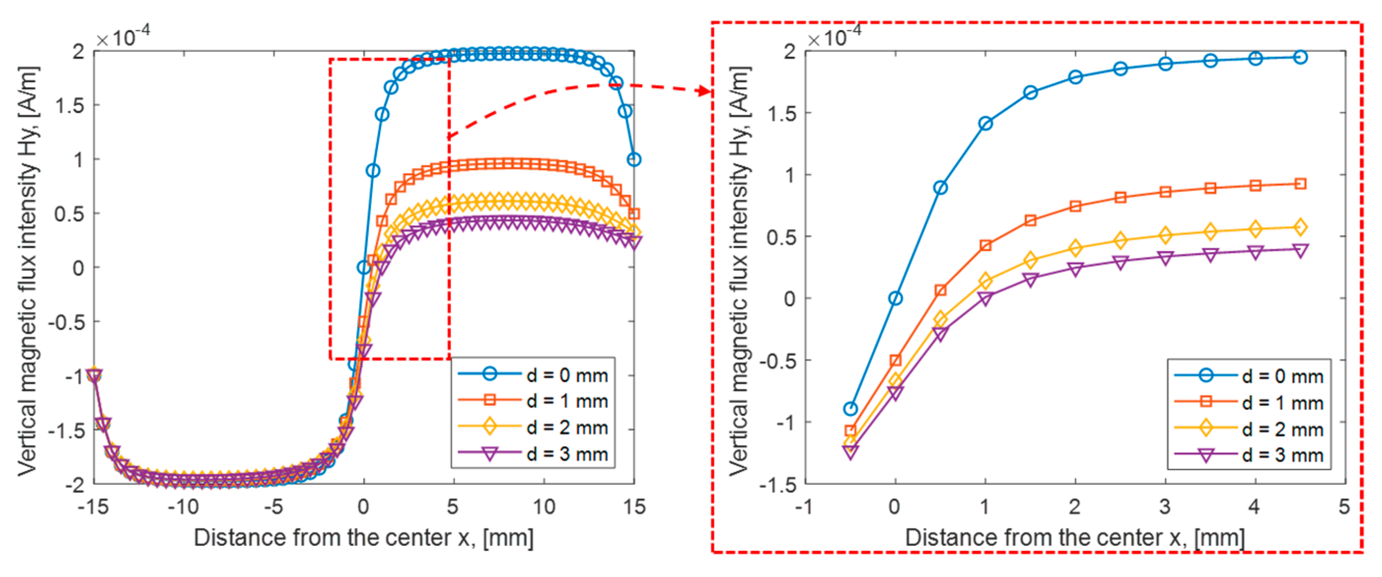
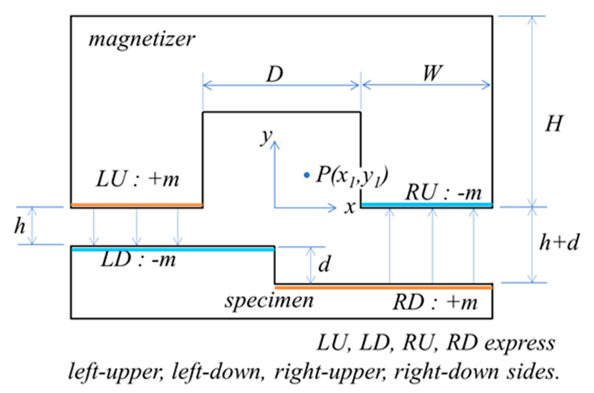
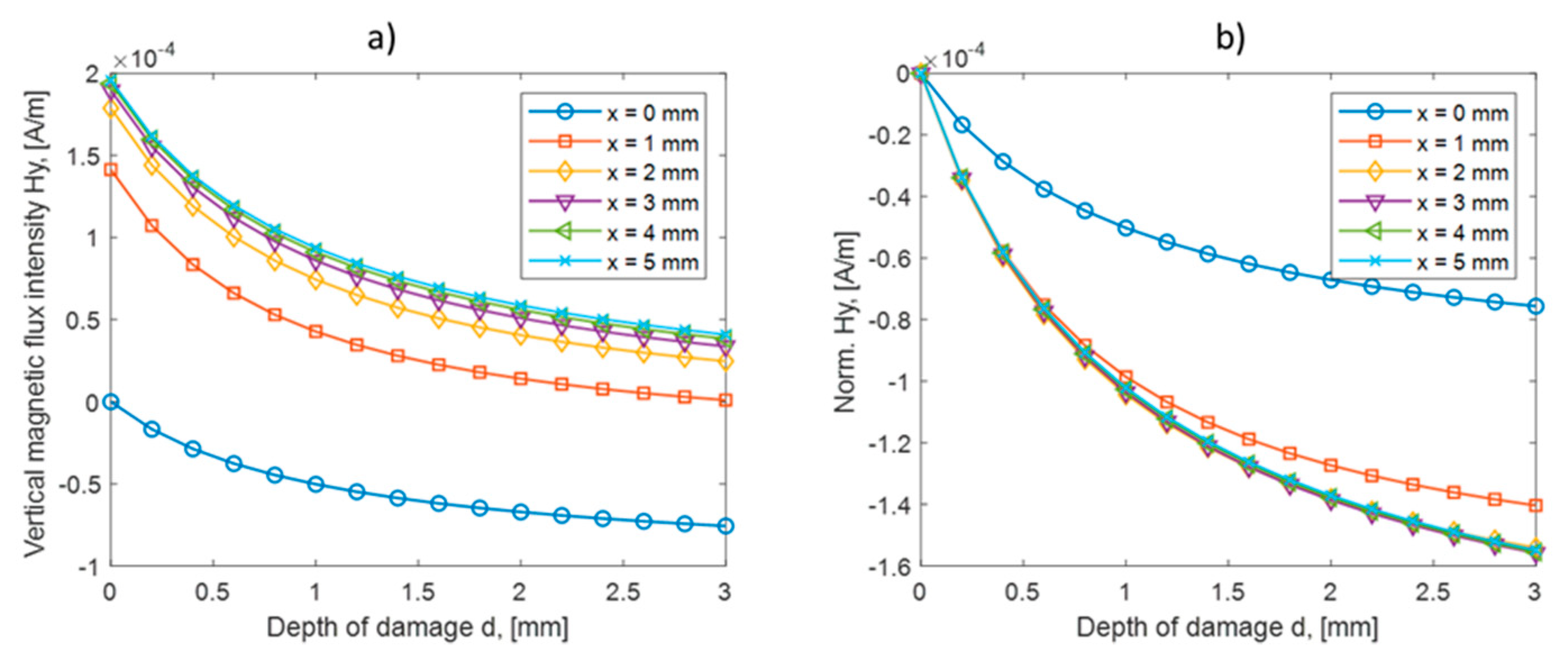
2.1. Measurement of Magnetic Flux Density
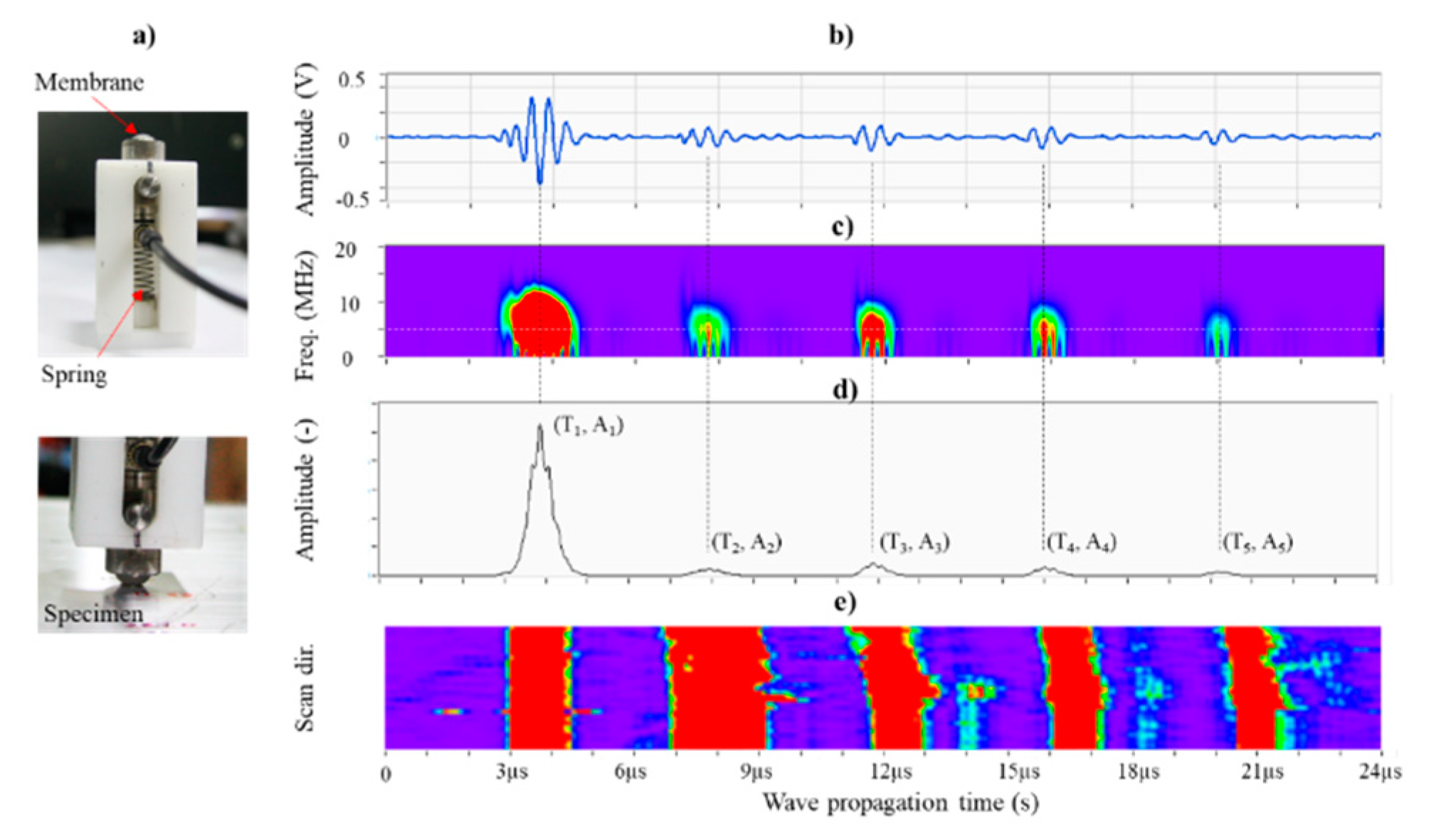
2.2. Flexible Ultrasonic Testing
3. Experiment and Results
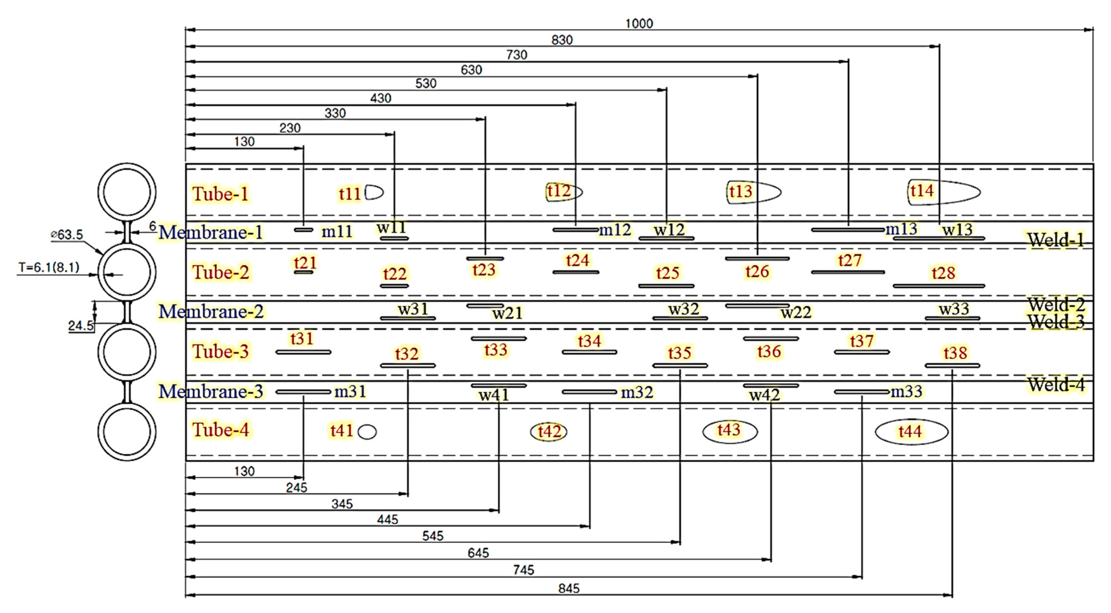
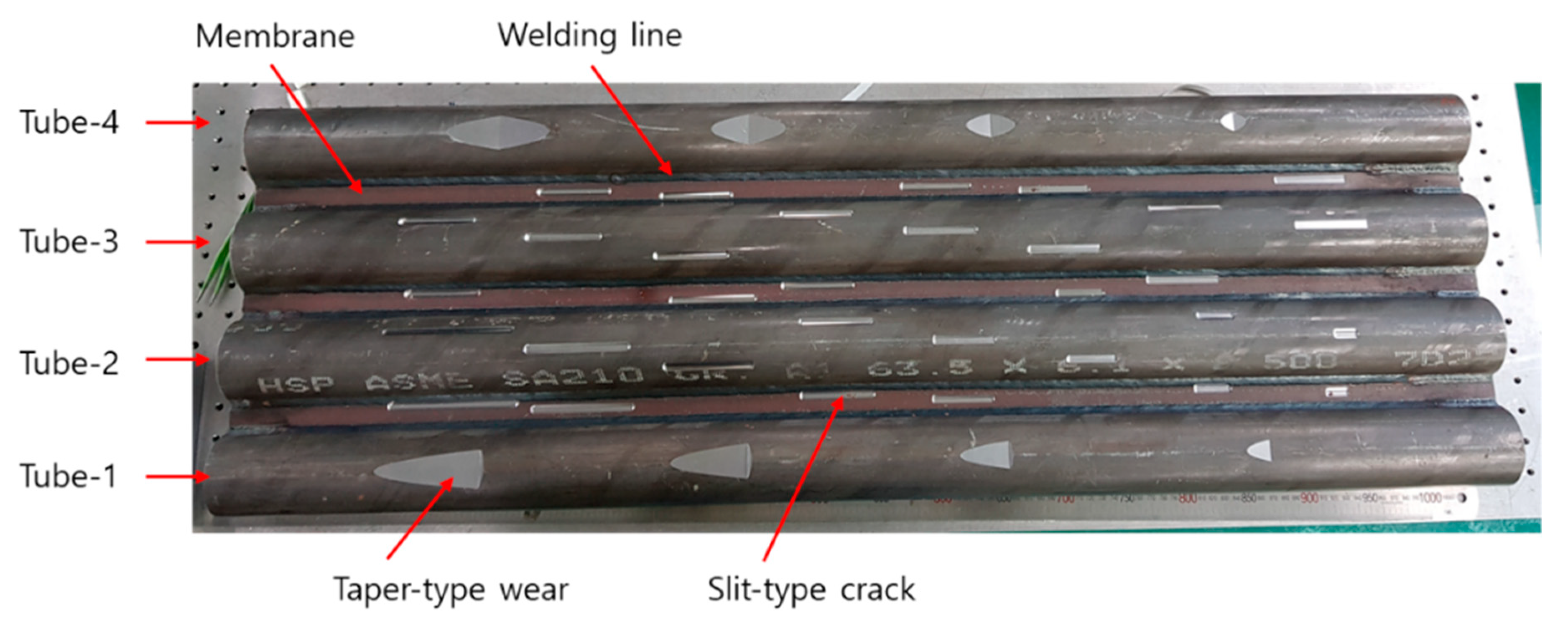
3.1. Specimen
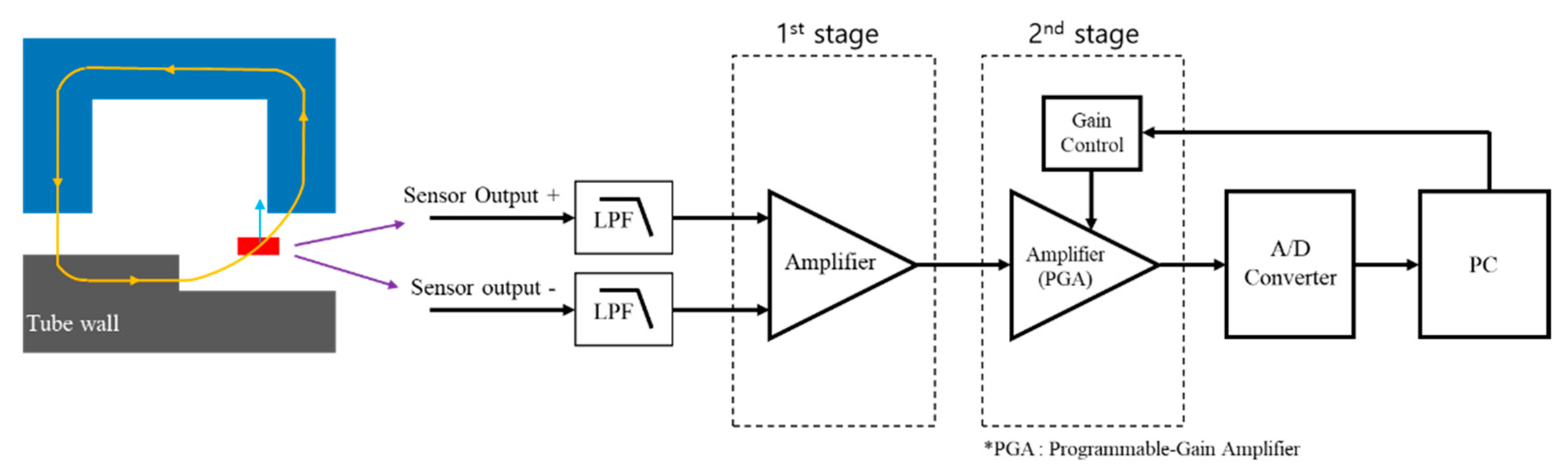
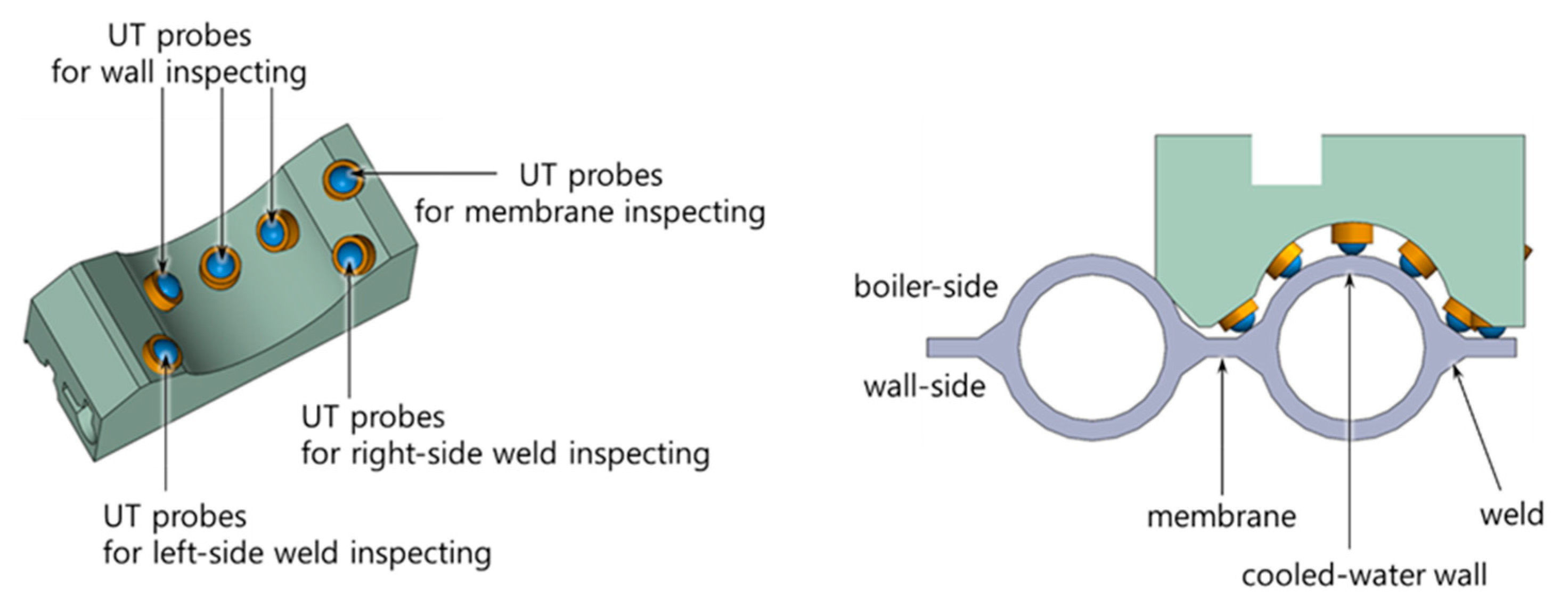
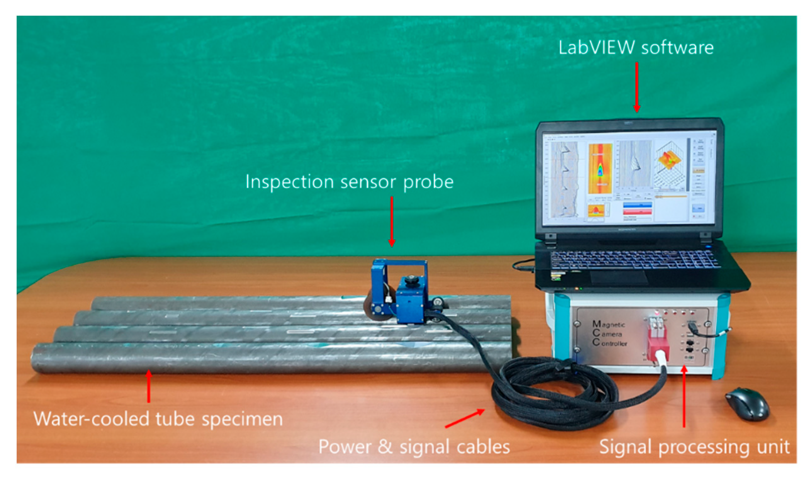
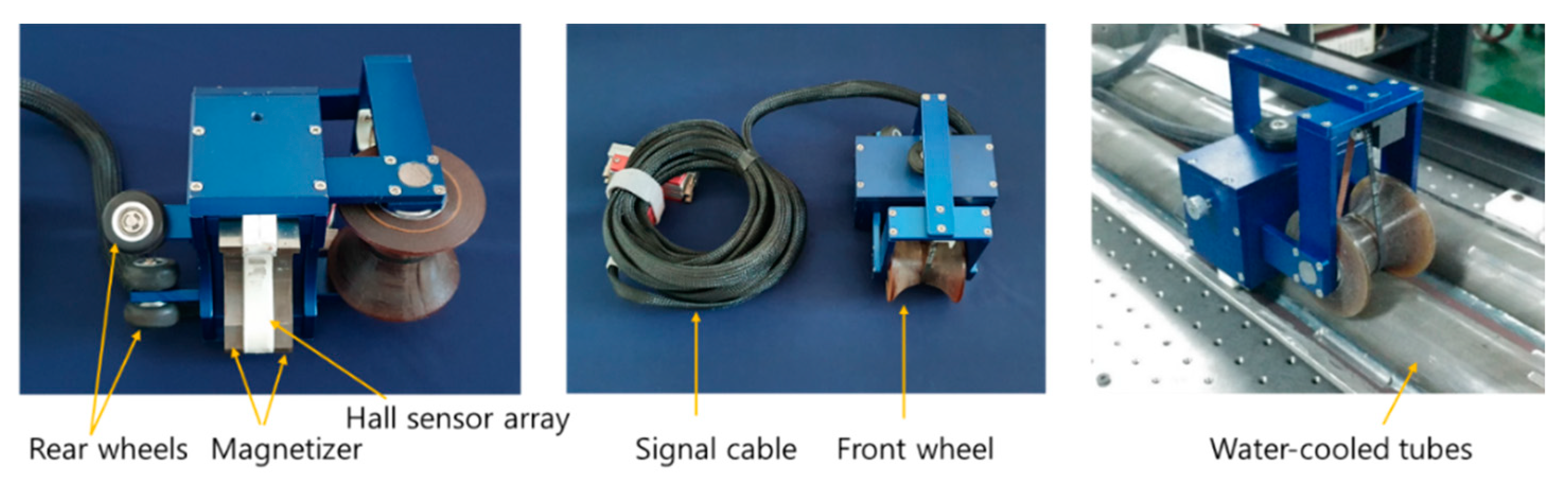
3.2. Inspection System
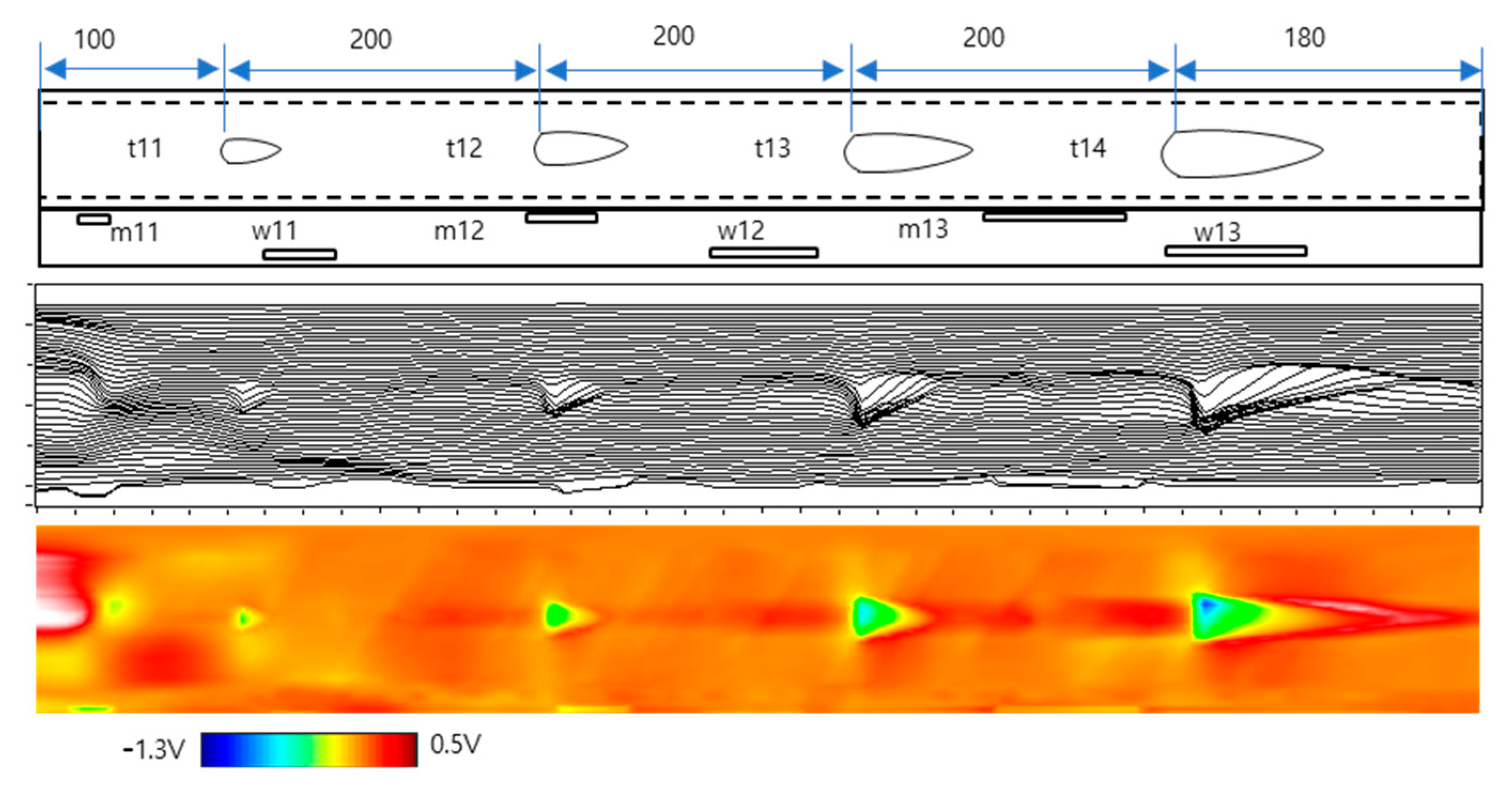
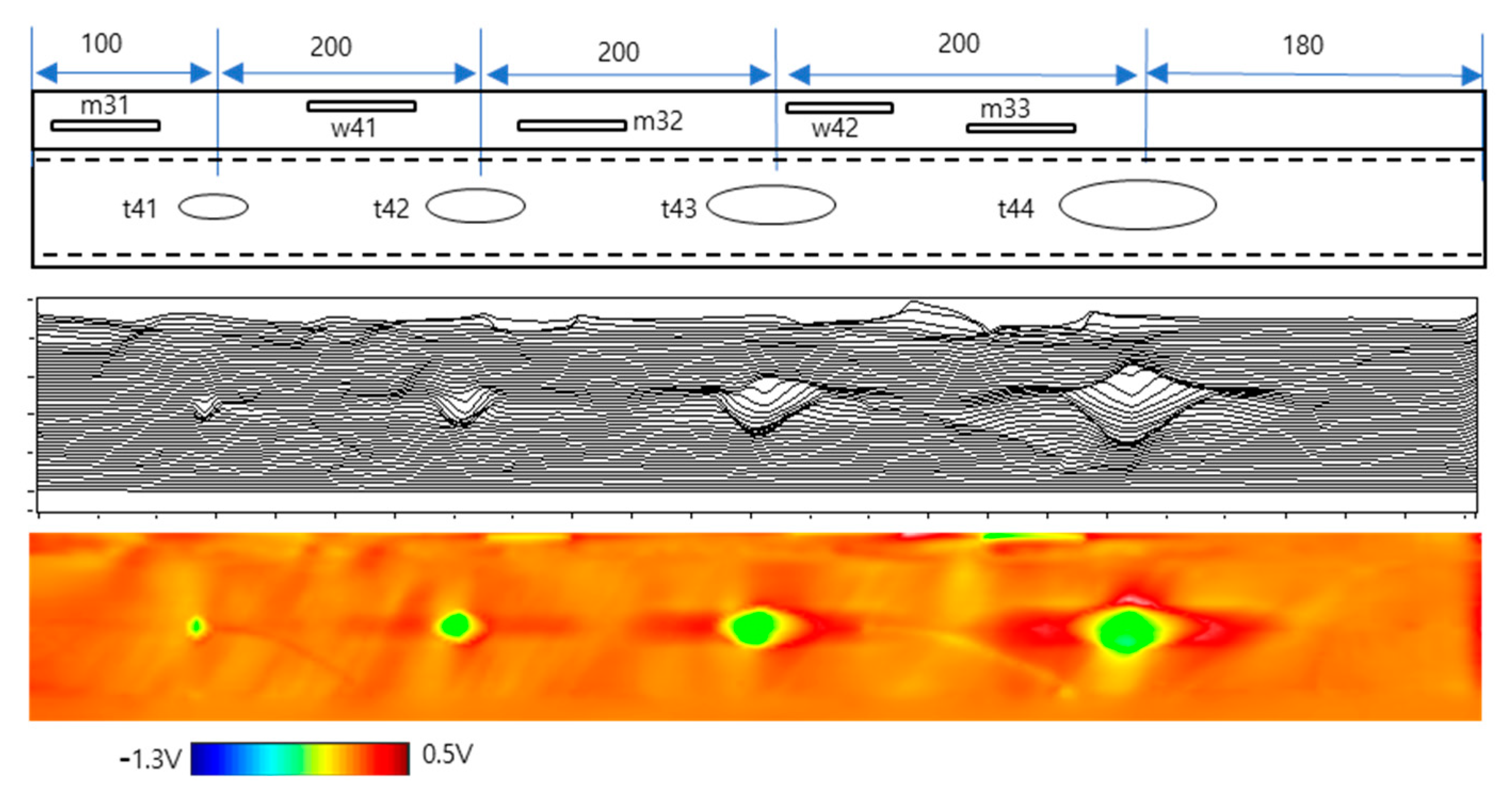
3.3. Experiment Results
4. Conclusions
Author Contributions
Funding
Conflicts of Interest
References
- Basu, P. Combustion of coal in circulating fluidized-bed boilers: A review. Chem. Eng. Sci. 1999, 54, 701–764. [Google Scholar] [CrossRef]
- Wang, B. Erosion-corrosion of thermal sprayed coatings in FBC boilers. Wear 1996, 199, 24–32. [Google Scholar] [CrossRef]
- Kim, T.-W.; Choi, J.-H.; Shun, D.-W.; Son, J.-E.; Jung, B.; Kim, S.-S.; Kim, S.-D. A Tube Thickness Map of Water Wall in a Commercial Circulating Fluidized Bed Combustor. Korean Chem. Eng. Res. 2005, 43, 412–418. [Google Scholar]
- Jung, M.-J.; Park, B.-C.; Bae, J.-H.; Shin, S.-C. PAUT-based defect detection method for submarine pressure hulls. Int. J. Nav. Archit. Ocean Eng. 2018, 10, 153–169. [Google Scholar] [CrossRef]
- Kim, Y.; Cho, S.; Park, I.K. Analysis of Flaw Detection Sensitivity of Phased Array Ultrasonics in Austenitic Steel Welds According to Inspection Conditions. Sensors 2021, 21, 242. [Google Scholar] [CrossRef] [PubMed]
- Yusa, N.; Chen, Z.; Miya, K. Quantitative profile evaluation of natural defects in a steam generator tube from eddy current signals. Int. J. Appl. Electromagn. Mech. 2000, 12, 139–150. [Google Scholar] [CrossRef]
- Xie, S.; Chen, Z.; Takagi, T.; Uchimoto, T. Evaluation of Wall Thinning in Carbon Steel Piping Based on Magnetic Saturation Pulsed Eddy Current Testing Method. Stud. Appl. Electromagn. Mech. 2013, 39, 296–303. [Google Scholar]
- Le, M.; Kim, J.; Kim, J.; Do, H.S.; Lee, J. “Electromagnetic testing of moisture separator reheater tubes using a bobbin-type integrated Hall sensor array. Int. J. Appl. Electromagn. Mech. 2017, 55, S203–S209. [Google Scholar] [CrossRef]
- Le, M.; Kim, J.; Kim, J.; Do, H.S.; Lee, J. Nondestructive testing of moisture separator reheater tubing system using Hall sensor array. Nondestruct. Test. Eval. 2018, 33, 35–44. [Google Scholar] [CrossRef]
- Lafontaine, G.; Hardy, F.; Renaud, J. X-Probe® ECT array: A high-Speed Replacement for Rotating Probes. In Proceedings of the Third International Conference on NDE in Relation to Structural Integrity for Nuclear and Pressurized Components, Seville, Spain, 14–16 November 2001. [Google Scholar]
- Joubert, P.Y.; Bihan, Y.L.; Placko, D. Localization of defects in steam generator tubes using a multi-coil eddy current probe dedicated to high speed inspection. NDT E Int. 2002, 35, 53–59. [Google Scholar] [CrossRef]
- Choi, C.D.; Lim, I.S. Comparative Reliability of Nondestructive Testing for Weld: Water Wall Tube in Thermal Power Plant Boiler Case Study. J. Appl. Reliab. 2018, 18, 240–249. [Google Scholar] [CrossRef]
- Vajpayee, A.; Russell, D. Automated Condition Assessment of Boiler Water Wall Tubes Using Remote Field Technology. A Revolution over Traditional and Existing Techniques. In Proceedings of the 10th International Conference of the Slovenian Society for Nondestructive Testing, Ljubljana, Slovenia, 1–3 September 2009; pp. 523–530. [Google Scholar]
- Gil, D.-S.; Jung, G.-J.; Seo, J.-S.; Kim, H.-J.; Kwon, C.-W. Simulation of Remote Field Scanner for Defect Evaluation of Water Wall Tube within the Fluidized Bed Boiler. KEPCO J. Electr. Power Energy 2020, 6, 145–150. [Google Scholar]
- Atherton, D.L.; Mackintosh, D.D.; Sullivan, S.P.; Dubois, J.M.S.; Schmidt, T.R. Remote-Field Eddy Current Signal Representation. Mater. Eval. 1993, 51, 782–789. [Google Scholar]
- Park, J.-H.; Yoo, H.-R.; Kim, D.-K.; Kim, H.-J.; Cho, S.-H.; Song, S.-J.; Kim, H.-M.; Park, G.-S.; Rho, Y.-W. Development of RFECT System for In-Line Inspection Robot Considering Extendibility of Receiving Senosors based on Parallel Lock-in Amplifer. Int. J. Precis. Eng. Manuf. 2017, 18, 145–153. [Google Scholar] [CrossRef]
- Park, J.W.; Park, J.H.; Song, S.J.; Kishore, M.B.; Kwon, S.G.; Kim, H.J. Enhanced Detection of Defects Using GMR Sensor Based Remote Field Eddy Current Techique. J. Magn. 2017, 22, 531–538. [Google Scholar] [CrossRef]
- Lee, H.; Choe, E.; Lee, J.; Jung, G. Magnetic Flux Leakage Measurement System for Nondestructive Testing of Water-Cooled Wall. In Proceedings of the 2019 IEEE International Instrumentation and Measurement Technology Conference (I2MTC), Auckland, New Zealand, 20–23 May 2019; pp. 1–5. [Google Scholar]
- Vakhguelt, A.; Kapayeva, S.D.; Bergander, M.J. Combination Non-Destructive Test (NDT) Method for Early Damage Detection and Condition Assessment of Boiler Tubes. Procedia Eng. 2017, 188, 125–132. [Google Scholar] [CrossRef]
- Kapayeva, S.D.; Bergander, M.J.; Vakhguelt, A.; Khairaliyev, S.I. Remaining life assessment for boiler tubes affected by combined effect of wall thinning and overheating. Int. J. Vibroeng. 2017, 19, 5892–5907. [Google Scholar] [CrossRef]
- Hwang, J.; Lee, J. Modeling of a Scan Type Magnetic Camera Image Using the Improved Dipole Model. J. Mech. Sci. Technol. 2006, 20, 1691–1701. [Google Scholar] [CrossRef]
- Lee, J.; Jun, J.W.; Hwang, J.S.; Lee, S.H. Development of Numerical Analysis Software for the NDE by using Dipole Model. Key Eng. Mater. 2007, 353–358, 2383–2386. [Google Scholar] [CrossRef]
- Le, M.; Kim, J.; Kim, S.; Lee, J. Nondestructive Testing of Pitting Corrosion Cracks in Rivet of Multilayer Structures. IJPEM 2016, 17, 1433–1442. [Google Scholar] [CrossRef]


| # | Width [mm] | Length [mm] | Depth (mm) | Position (mm) | # | Width [mm] | Length [mm] | Depth (mm) | Position (mm) |
|---|---|---|---|---|---|---|---|---|---|
| Tube-1 (One-Side Taper-Type Wear) | Tube-4 (Two-Side Taper-Type Wear) | ||||||||
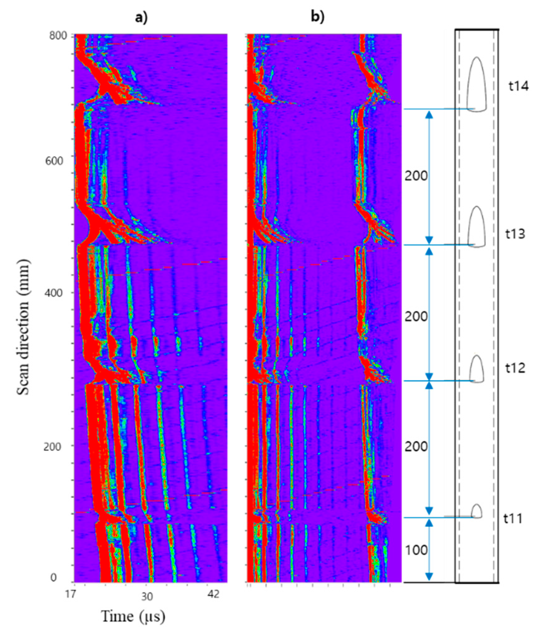
| t11 | 16 | 20 | 0.9 | 200 | t41 | 16 | 20 | 0.9 | 200 |
| t12 | 20 | 40 | 1.5 | 400 | t42 | 20 | 40 | 1.5 | 400 |
| t13 | 25 | 60 | 2.5 | 600 | t43 | 25 | 60 | 2.5 | 600 |
| t14 | 28 | 80 | 3.1 | 800 | t44 | 28 | 80 | 3.1 | 800 |
| # | Width [mm] | Length [mm] | Depth (mm) | Position (mm) | # | Width [mm] | Length [mm] | Depth (mm) | Position (mm) |
|---|---|---|---|---|---|---|---|---|---|
| Tube-2 (Same Width) | Tube-3 (Same Length) | ||||||||
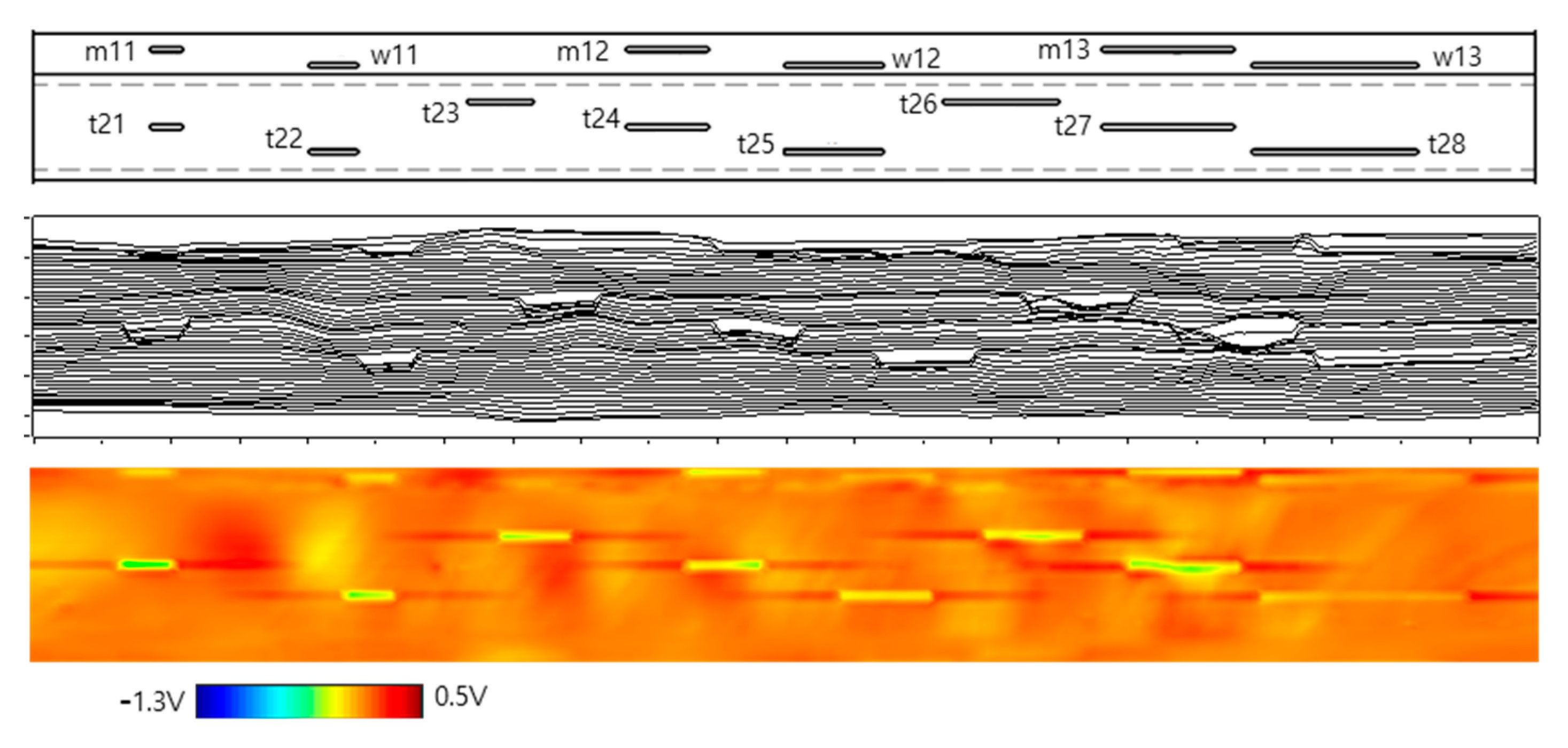
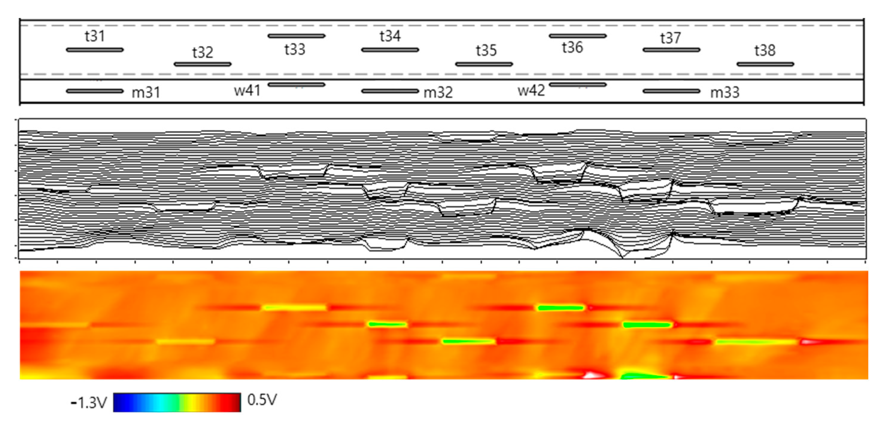
| t21 | 7 | 20 | 0.9 | 130 | t31 | 7 | 60 | 0.23 | 130 |
| t22 | 7 | 30 | 0.9 | 230 | t32 | 7 | 60 | 0.50 | 245 |
| t23 | 7 | 40 | 0.9 | 330 | t33 | 7 | 60 | 0.96 | 345 |
| t24 | 7 | 50 | 0.9 | 430 | t34 | 7 | 60 | 1.08 | 445 |
| t25 | 7 | 60 | 0.9 | 530 | t35 | 7 | 60 | 1.5 | 545 |
| t26 | 7 | 70 | 0.9 | 630 | t36 | 7 | 60 | 1.86 | 645 |
| t27 | 7 | 80 | 0.9 | 730 | t37 | 7 | 60 | 2.34 | 745 |
| t28 | 7 | 100 | 0.9 | 830 | t38 | 7 | 60 | 2.64 | 845 |
| # | Width [mm] | Length [mm] | Depth (mm) | Position (mm) | # | Width [mm] | Length [mm] | Depth (mm) | Position (mm) |
|---|---|---|---|---|---|---|---|---|---|
| Membrane-1 | Membrane-3 | ||||||||
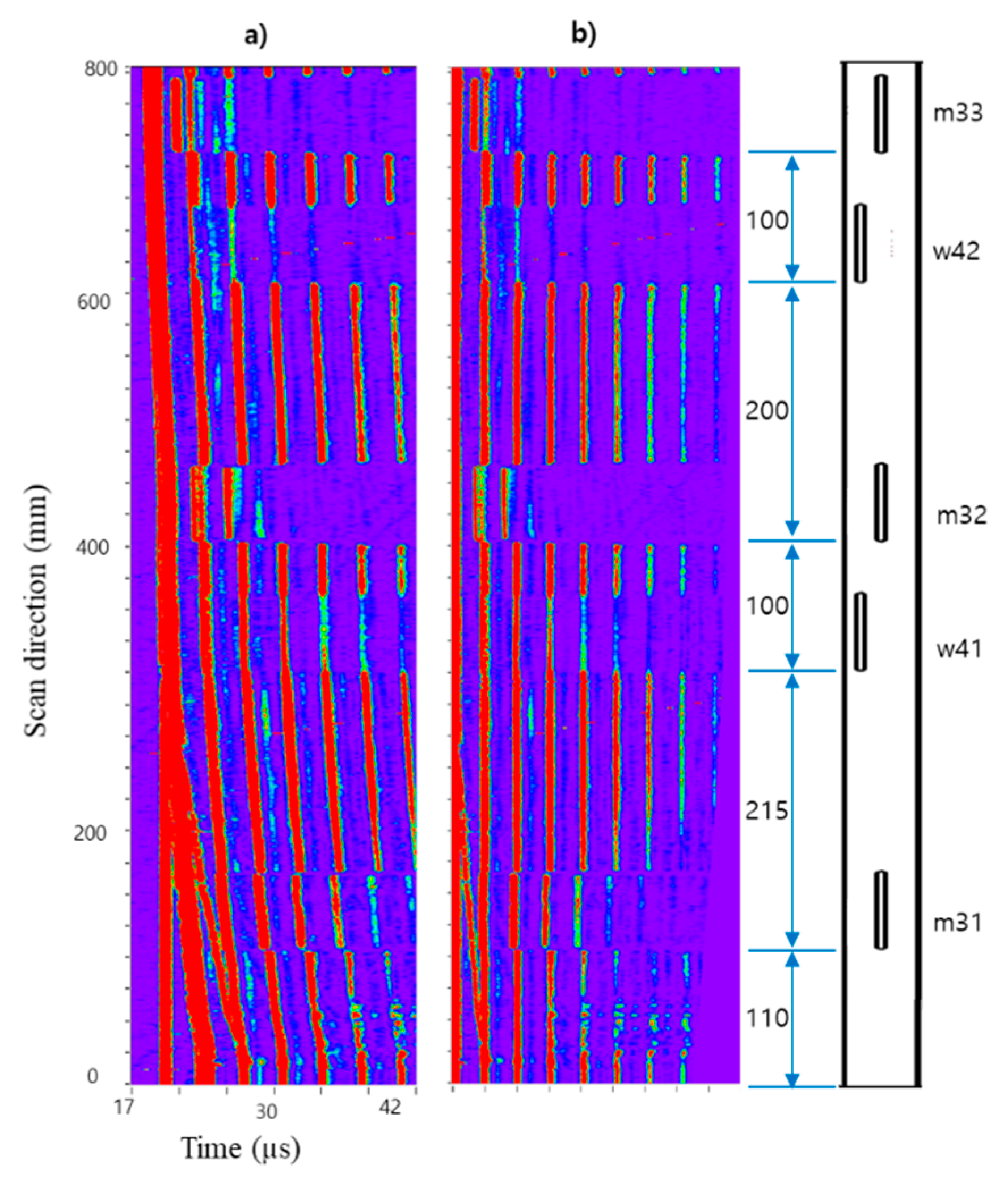
| m11 | 7 | 20 | 0.9 | 130 | m31 | 7 | 60 | 0.3 | 130 |
| m12 | 7 | 50 | 0.9 | 430 | m32 | 7 | 60 | 1.2 | 445 |
| m13 | 7 | 80 | 0.9 | 730 | m33 | 7 | 60 | 2.4 | 745 |
| # | Width [mm] | Length [mm] | Depth (mm) | Position (mm) | # | Width [mm] | Length [mm] | Depth (mm) | Position (mm) |
|---|---|---|---|---|---|---|---|---|---|
| Weld-1 | Weld-3 | ||||||||
| w11 | 7 | 30 | 0.9 | 230 | w31 | 7 | 60 | 0.6 | 245 |
| w12 | 7 | 60 | 0.9 | 530 | w32 | 7 | 60 | 1.5 | 545 |
| w13 | 7 | 100 | 0.9 | 830 | w33 | 7 | 60 | 3.0 | 845 |
| Weld-2 | Weld-4 | ||||||||
| w21 | 7 | 40 | 0.9 | 330 | w41 | 7 | 60 | 0.9 | 345 |
| w22 | 7 | 70 | 0.9 | 630 | w42 | 7 | 60 | 1.8 | 645 |
Publisher’s Note: MDPI stays neutral with regard to jurisdictional claims in published maps and institutional affiliations. |
© 2021 by the authors. Licensee MDPI, Basel, Switzerland. This article is an open access article distributed under the terms and conditions of the Creative Commons Attribution (CC BY) license (http://creativecommons.org/licenses/by/4.0/).
Share and Cite
Lee, J.; Choe, E.; Pham, C.-T.; Le, M. Measurement of Thinned Water-Cooled Wall in a Circulating Fluidized Bed Boiler Using Ultrasonic and Magnetic Methods. Appl. Sci. 2021, 11, 2498. https://doi.org/10.3390/app11062498
Lee J, Choe E, Pham C-T, Le M. Measurement of Thinned Water-Cooled Wall in a Circulating Fluidized Bed Boiler Using Ultrasonic and Magnetic Methods. Applied Sciences. 2021; 11(6):2498. https://doi.org/10.3390/app11062498
Chicago/Turabian StyleLee, Jinyi, Eunho Choe, Cong-Thuong Pham, and Minhhuy Le. 2021. "Measurement of Thinned Water-Cooled Wall in a Circulating Fluidized Bed Boiler Using Ultrasonic and Magnetic Methods" Applied Sciences 11, no. 6: 2498. https://doi.org/10.3390/app11062498
APA StyleLee, J., Choe, E., Pham, C.-T., & Le, M. (2021). Measurement of Thinned Water-Cooled Wall in a Circulating Fluidized Bed Boiler Using Ultrasonic and Magnetic Methods. Applied Sciences, 11(6), 2498. https://doi.org/10.3390/app11062498