Article

Experimental Assessment of RANS Models for Wind Load Estimation over Solar-Panel Arrays

Aerospace Engineering Research Group, Universidad Carlos III de Madrid, Avenida de la Universidad 30, 28911 Leganés, Spain
*
Author to whom correspondence should be addressed.
Appl. Sci. 2021, 11(6), 2496; https://doi.org/10.3390/app11062496
Submission received: 24 February 2021 / Revised: 5 March 2021 / Accepted: 5 March 2021 / Published: 11 March 2021

Abstract

:
This paper reports a comparison between wind-tunnel measurements and numerical simulations to assess the capabilities of Reynolds-Averaged Navier-Stokes models to estimate the wind load over solar-panel arrays. The free airstream impinging on solar-panel arrays creates a complex separated flow at large Reynolds number, which is severely challenging for the current Reynolds-Averaged Navier-Stokes models. The Reynolds-Averaged Navier-Stokes models compared in this article are k- ϵ , Shear-Stress Transport k- ω , transition and Reynolds Shear Model. Particle Image Velocimetry measurements are performed to investigate the mean flow-velocity and turbulent-kinetic-energy fields. Pressure taps are located in the surface of the solar panel model in order to obtain static pressure measurements. All the Reynolds-Averaged Navier-Stokes models predict accurate average velocity fields when compared with the experimental ones. One of the challenging factor is to predict correctly the thickness of the turbulent wake. In this aspect, Reynolds Shear provides the best results, reproducing the wake shrink observed on the 3rd panel in the experiment. On the other hand, some other features, most notably the blockage encountered by the flow below the panels, are not correctly reproduced by any of the models. The pressure distributions over the 1st panel obtained from the different Reynolds-Averaged Navier-Stokes models show good agreement with the pressure measurements. However, for the rest of the panels Reynolds-Averaged Navier-Stokes fidelity is severely challenged. Overall, the Reynolds Shear model provides the best pressure estimation in terms of pressure difference between the front and back sides of the panels.

1. Introduction

Solar panels are generally designed to withstand a frontal wind with predetermined intensity [1]; load reduction due to the arrangement of the elements of a solar-panel array is not considered in the design phase. In a solar-panel array, the first panel row deflects the incoming wind, producing a separated and turbulent wake that impacts against the following panels. Due to shielding effect, the other rows may benefit of smaller (on average) structural loads, but are also likely to be subjected to unsteady forces generated in the wake. More robust predictions of wind loads on solar panels would allow a reduction of the maintenance costs and of the manufacturing price of the support structure. This costs reduction will improve the competitive capacity of this type of energy.
Timilsina et al. [2] have shown that, due to capital costs, the current market price of solar power is still higher than what could be achieved by conventional systems (e.g., nuclear, coal, gas). Nevertheless solar energy might become competitive in the short future. Geyer et al. [3] identified a possible strategy to cut the capital cost of solar arrays in the simplification of the panels design and thus in their structural optimization. Additionally, wind loads might add on top of other climate parameter (such as temperature, humidity, etc., see e.g., [4]) affecting the aging and performance degradation of photo-voltaic panels [5,6,7]. In this frame, a proper characterisation of the wind loads on panel arrays must be performed, also considering that these loads are far from being negligible. In the recent years, in fact, solar panels have become a quite popular solution in small communities to achieve energy independence or, in extended power grids, to provide a distributed energy resource nearby load centers, therefore cutting the energy transmission and distribution costs. In these applications, panels are typically mounted on building rooftops, where they have to face sustained winds. The flow field and loads affecting rooftop-mounted solar panels have been analyzed by several studies in the literature [8,9,10,11].
Both numerical [12,13,14,15,16] and experimental [17,18,19,20] studies have been carried out in order to analyse the wind loads on solar panels in both single- and multiple-array configuration. Bitsuamlak et al. [12] performed simulations both on a single panel and on a three-panels array. The simulations consisted of an initial run using Reynolds-Averaged Navier-Stokes (RANS) simulation, aimed at obtaining reliable initial conditions, followed by a run using Large-Eddy Simulation (LES). Their results showed that the magnitude of the pressure coefficients was generally underestimated by the numerical calculations when compared to the experimental results, although the same patterns of pressure coefficient distribution was found. The study also provides evidence of the shielding effect. Shademan and Hangan [13] performed several RANS simulations with k- ϵ , k- ω and Reynolds-Stress Model (RSM) turbulence closure models. The study analyzed the flow field around a single solar panel for different wind direction and different panel inclinations. Their results showed that the critical cases for the loads on the solar panel correspond with the wind direction 0 and 180 . Shademan et al. [14] also performed RANS simulations with Shear-Stress Transport (SST) k- ω and k- ϵ closure models discretising the solar panel into a 2 × 2 sub-panels and varying the gap between them. Their results showed that bottom panels experience larger mean wind loading compared to the top panels. Although the introduction of gap spacing results in reduced mean wind forces, it produces regions that experience larger wind loading. Moreover, the increase of the ground clearance also causes larger mean wind loading on the panels. Jubayer and Hangan [15] performed a RANS simulation with SST k- ω closure models. This study showed that the the front panel always experiences the maximum loads, but the wind direction may affect the loads on the following panels.
Although single-panel studies provide relevant design information, the array configuration has been found to strongly modify the load distribution. Chevalier and Norton [17] demonstrated experimentally that the front panel in an array absorbs less force than the equivalent isolated panel, and that the subsequent panels receive loads which depend upon the pitch ratio. Abiola-Ogedengbe et al. [18] conducted an experimental study to investigate the pressure field on the upper and lower surface of a single panel. The separation between panels has an influence on surface pressure field, specifically the one of the front panel, but the orientation of the panel relative to the wind also plays a role in altering the influence of panel distance on the surface pressure field. García et al. [19] performed an experimental campaign with parabolic troughs collectors protected by windbreaks (solid wall and porous fence). They concluded that with the appropriate selection of design parameters it is possible to reduce the aerodynamic loads (mean and peaks values) up to 60% over the first row of parabolic troughs collectors.
Even if RANS simulations still represent the backbone of flow modelling in industrial applications, they are severely challenged in scenarios like the one that is object of the present study, i.e., turbulent/transitional flows with with flow separation and reattachment [21]. Currently, transition SST and SST k- ω [22,23,24] are the RANS closure model more frequently used to simulate this type of flows. Three-dimensional steady RANS models, like k- ϵ , have been used to obtain mean wind-velocity pattern [25]. The assessment of the uncertainty produced by these models, however, has not been thoughtfully discussed for panels-array problems. As an example, a similar discussion has been tackled by Catalano et al. [26] for the transonic flow over an airfoil, using wind-tunnel data as a reference.
The objective of present work is to assess the modelling capabilities of different RANS models to estimate the wind loads over solar-panel arrays. Provided that the typical angle of attack of the panels with respect to the wind is sufficiently large (which is often the case for solar-panel arrays, with typical inclination of 45 ), an experimental campaign in a wind tunnel has been carried out on a simplified mock-up of a solar-panel array with the purpose of providing a solid experimental dataset, assessing the robustness of RANS models in such scenario. The Reynolds number based on panel-chord length is 4.0 × 10 4 . The panel array configuration and boundary conditions that have been used in the experimental setup have been reproduced in the numerical simulations performed with the selected RANS models.
The paper is organized as follows. After describing the experimental set-up and the post-processing techniques in Section 2, the numerical models are summarized in Section 3. Section 4 shows the main experimental and numerical results and a discussion on their comparison. Finally, in Section 5, the main conclusions of the study are presented.

2. Experimental Set-Up

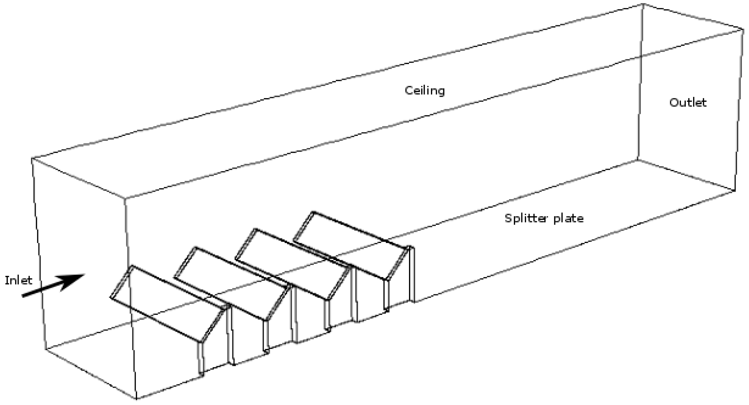
The experimental study has been carried out in the closed-loop wind tunnel of the Aerospace Engineering Group at the Universidad Carlos III de Madrid. The test section of this wind tunnel has a square cross area of 0.4 m × 0.4 m with a length of 1.5 m. The ceiling and the lateral walls of the tunnel are made of transparent methacrylate in order to enable optical access. Free-stream turbulence intensity is estimated to be lower than 1% by means of Particle Image Velocimetry (PIV) measurements in the empty tunnel. A flat plate with length of 0.55 m equipped with a sharp leading edge is installed in the test section. The solar-panel array is mounted on top of this plate instead of the tunnel floor in order to reproduce ground effect with a relatively thin boundary layer. The solar-panel array is composed of four panels, each with chord length c of 0.05 m, thickness t of 0.005 m and span l of 0.4 m. The panels are inclined of 45 with respect to the ground. The pitch between the panels is 2 c. The first panel is located at a distance of 2 c from the leading edge of the flat plate. The leading edge of the 4th panel is 3 c away from the trailing edge of the flat plate in order to reduce the effect of the flat plate end. Figure 1 shows a sketch of the experimental setup. The wind tunnel velocity, U , at the test-section inlet is kept constant and equal to 12.8 m/s for all the experiments in order to achieve a Reynolds number based on the panel chord of about 4.0 × 10 4 , thus being in the turbulent regime.
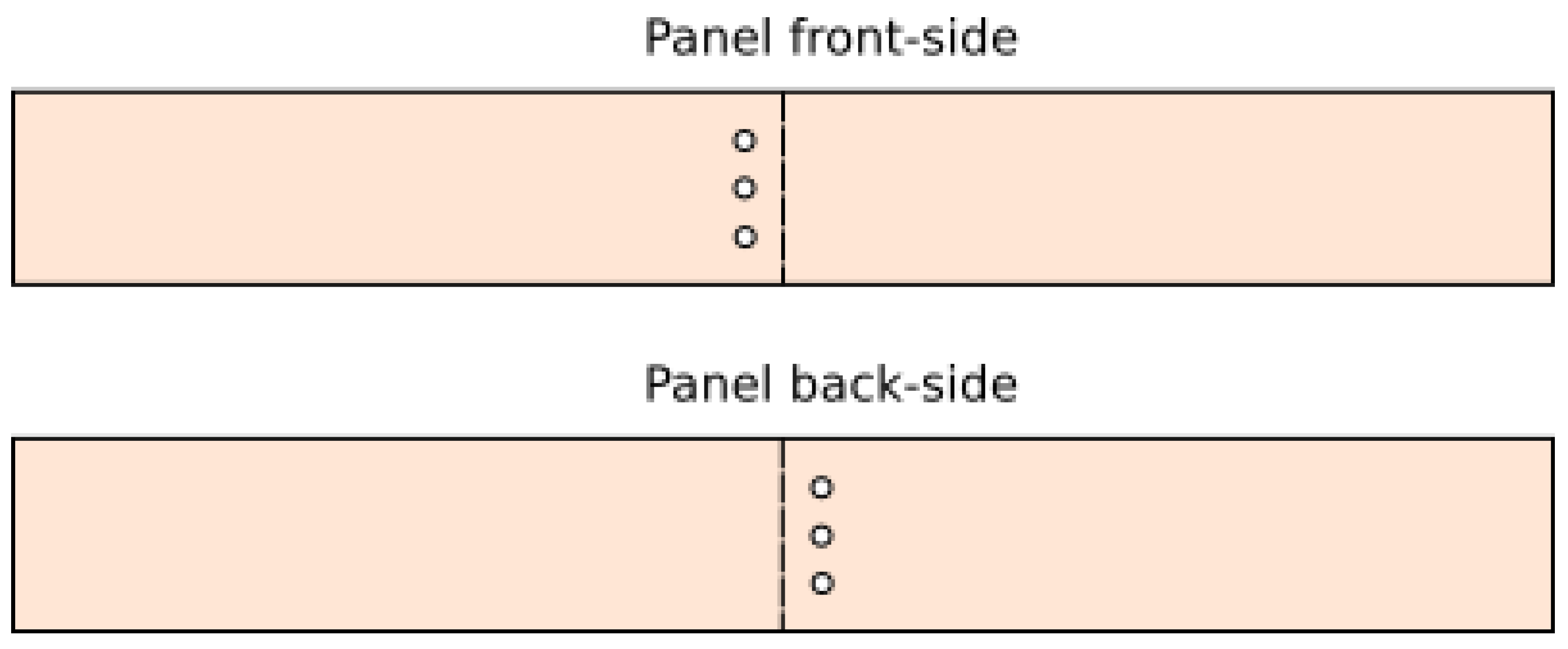
Each panel is equipped with 6 pressure taps, 3 on the front side and 3 on the back side, approximately located in the mid-span section. On each side the pressure taps are positioned in the chord-wise direction at 0.25 c, 0.50 c and 0.75 c. Front and back taps are displaced of 0.20 c along the span-wise direction with respect to the mid section, respectively on the left and on the right (the total distance between front and back taps is 0.40 c). Each tap has a 1.2 mm diameter. Figure 2 shows a schematic of the pressure taps location on the solar panels. Pressure measurements are performed with a tube system that connects the pressure taps located on the model surface to a pressure transducer. The pressure transducer used in the experiment has an uncertainty of 0.011 in terms of pressure coefficient C p = p p 0.5 ρ U 2 , being ρ and p the ambient air density and pressure respectively. An ensemble of 10,000 measurements is acquired for each pressure tap, thus reducing the uncertainty on the average pressures to 0.00011 in terms of the pressure coefficient.
Velocity field measurements are acquired by means of Particle Image Velocimetry (PIV). The flow is seeded with Di-Ethyl-Hexyl-Sebacate droplets with diameter of approximately 1 m. The light source is a Big Sky Laser CFR400 ND:Yag (230 mJ/pulse, pulse duration 3 ns). The acquisition is performed with a Andor Zyla 5.5 Camera (2650 × 2160 pixel array, 16.4 mm × 14 mm sensor size) with a spatial resolution of about 8.5 pixels/mm and a delay between pulses equal to 90 s. The sampling frequency of the PIV measurements is 10 Hz. An ensemble of 2000 image pairs is acquired for each experiment.
Image quality is improved with a background removal technique based on proper orthogonal decomposition (POD) [27]. This technique allows to remove laser reflections and illumination background, resulting in unbiased measurements near the wall.
The SPIV software, developed at University of Naples Federico II, is used to cross-correlate particle images and to calculate the velocity fields [28,29]. The interrogation strategy is an iterative multi-step image deformation algorithm, with final interrogation windows of 16 × 16 pixels, 50% overlap, resulting in a spatial resolution of 50 independent vectors per chord. The vector validation is carried out with a universal median test [30] on a 3 × 3 vectors kernel and a threshold equal to 2 is used to identify invalid vectors. Discarded vectors are replaced with a distance-weighted average of neighbour valid vectors. PIV uncertainty in the present case is mostly associated with random errors, for which a typical figure of merit of 0.1 pixels can be estimated in terms of the particle displacement error [31]. This results in an uncertainty of 1% of the free-stream velocity in the instantaneous velocity fields and of 0.05% of the free-stream velocity in the averaged velocity field.
Owing to the limited size of the camera sensor, the average field is computed by merging data from 3 different separate PIV experiments at three stations. The investigated fields of view are partially overlapped. The merging of the fields is carried out using a weighted average in the overlapping regions.
The data have been masked to remove regions where PIV measurements could not be carried out due to shadows of the panel along the laser path. These regions are covered in the following section with a white mask, while the lateral profiles of the solar panels are shown in black.

3. Numerical Model

RANS simulations have been carried out in a three-dimensional computational domain reproducing the wind-tunnel test section. Due to symmetry, the domain spans the half-width of the tunnel (0.2 m), while the height is equal to 0.26 m in order to reproduce the flat-plate/ceiling distance of the wind-tunnel experiment. The length of the domain is set to 1.1 m, long enough ensure that the boundary conditions do not affect the results on the region of interest. The leading edge of the first panel in the array having a distance of 0.1 m from the upstream boundary of the domain located at the leading edge of the flat plate. In order to reduce the mesh size, symmetry has been applied along the longitudinal-vertical plane of the computational domain. Figure 3 shows the contour of the computational domain used for the simulations.
Non-slip boundary conditions have been applied on the walls, ceiling and floor of the domain, as well as on the panel surfaces. Pressure outlet condition has been applied at the downstream boundary, with a temperature of 300 K and a static pressure of 101,325 Pa, while inlet velocity condition matching the one obtained from the experiments has been applied at the upstream boundary. The inlet velocity profile is set to match the PIV measurements. The simulation is initialized using the initialization algorithm available in ANSYS-Fluent.
The assessment has been carried out on four different RANS closure models. The first closure model is the k- ϵ model [32]. It uses two transport equations, one for the turbulent kinetic energy k, and one for the turbulent dissipation rate ϵ . This model assumes that the flow is fully turbulent, and thus the effects of molecular viscosity can be neglected. The second closure model assessed is the SST k- ω model [23]. It puts together the robust and accurate formulation of the k- ω model in the near-wall regions with the free-stream independence of k- ϵ model far from the wall [33]. The model works in such a way that k- ω model [34] is activated in the near-wall region. The third closure model assessed, the transition SST model [35], was originally proposed as a variation of the SST k- ω model. It is a four-equation model based on the coupling of the SST k- ω model with two additional transport equation, one for the intermittency and one for the transition onset criteria, in terms of momentum-thickness Reynolds number. All three aforementioned closure models rely on the Boussinesq hypothesis to model the Reynolds stresses ( ρ u i u j ¯ ), where the Reynolds decomposition of the velocity field ( u = U + u ) is used to refer to the mean (U) and fluctuating quantities ( u ) and the subscripts i and j indicate the velocity component according to the Einstein notation. This hypothesis assumes the eddy viscosity μ t as an isotropic scalar quantity in the Reynolds stresses equation, defined as:
ρ u i u j ¯ = μ t u i x j + u j x i 2 3 ρ k + μ t u k x k .
This assumption works well for flows dominated by only one of the Reynolds stresses. However, when these model are used to simulate complex flows with high degree of anisotropy, like separated wake after solar panels, the results are not satisfactory [36].
The fourth and last closure model assessed in this study is the Reynolds Stress Model (RSM), developed by Launder et al. [37] on the basis on the works of Chou [38] and Rotta [39]. It is characterised by solving all the components of the turbulent transport, instead of relying on the Boussinesq hypothesis. In all the cases, the turbulent intensity has been chosen as a 2.53% and as length scale 0.45 m, equivalent to the hydraulic diameter of the test chamber. In the next section, the following symbols are used to identify the correspondent model: k- ϵ ( Applsci 11 02496 i001); SST k- ω ( Applsci 11 02496 i002); transition SST ( Applsci 11 02496 i003); and RSM (▪▪▪▪▪▪▪).
A grid-mesh independence study was conducted to ensure on the independence of the results of the cell size. The study is performed starting with the initial mesh of 9 million elements, and using the refinement by gradients function in Fluent. In particular, the mesh have been refined where the largest normalized velocity gradients are found. After 6 refinement steps a final mesh of 38 million cells is used in the following. The mesh refinement study was stopped here since the difference in forces in the panels between the previous refinement step (24 Mcells) and the final mesh was smaller than a 0.5%, so it was decided that a following refinement was not needed.

4. Results

4.1. Mean Velocity Field

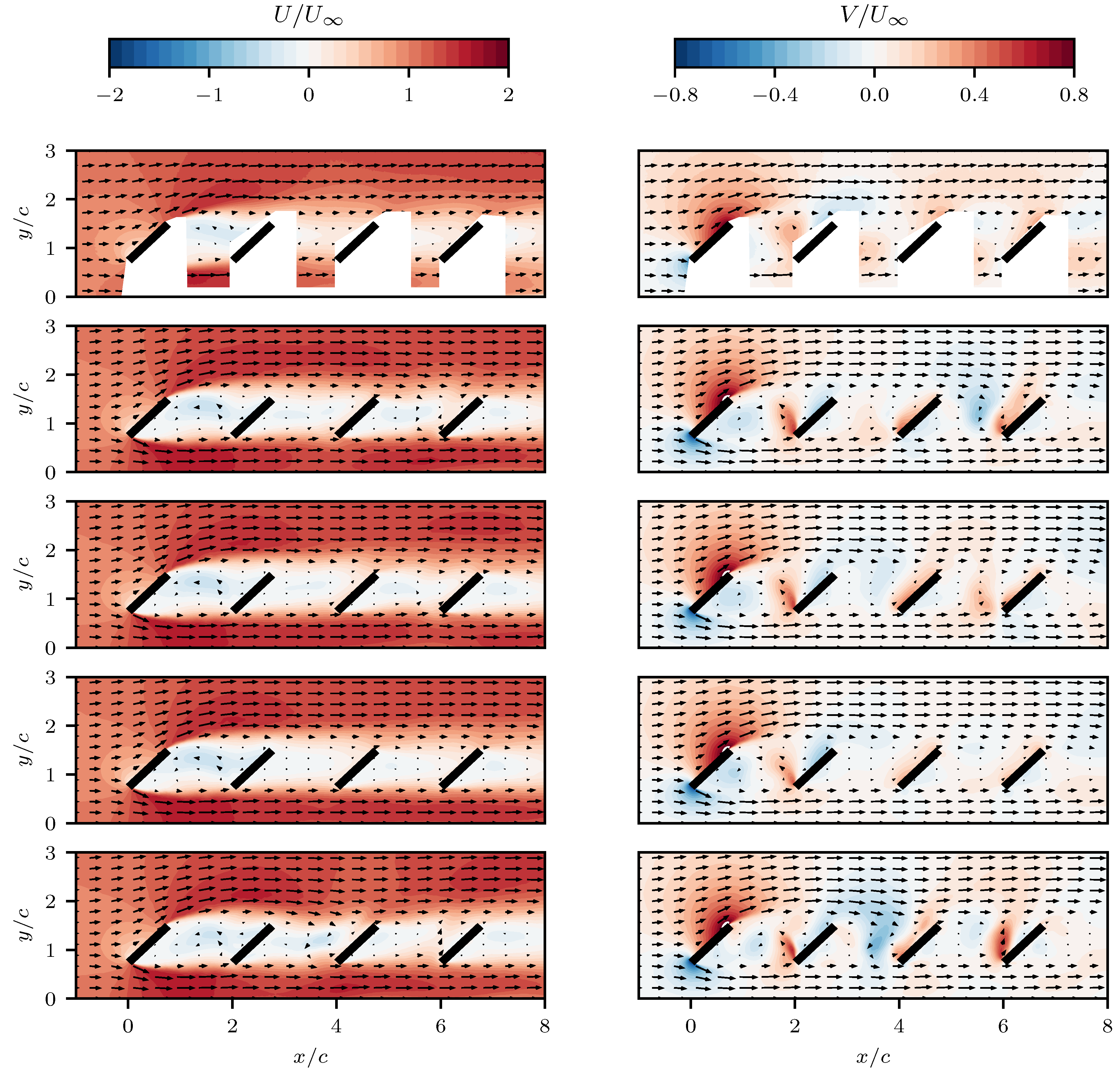
Figure 4 reports contour plots of both experimental and numerical results for the average streamwise U (left column) and vertical V (right column) velocity components. All velocities are scaled with U .
When the flow encounters the 1st panel, most of it is deflected upwards because of the panel inclination. The experimental results show that the mean vertical velocity increases over the 1st panel, reaching U exactly when leaving at the top corner of the panel. This behaviour is correctly reproduced by the four numerical simulations. With respect to the flow passing under the panel, the information that can be extracted from the experiment is limited due to the presence of the panel shadow. Nevertheless, it is possible to observe that the mean vertical velocity decreases up to almost - U at the bottom corner. This effect as well is correctly reproduced by all the numerical simulations.
Apart from the flow deflection over the 1st panel, both experiments and RANS simulations show that the mean streamwise velocity of the flow is accelerated up to 1.5 U when leaving the top corner of the 1st panel due to the blockage produced by the panel. However, experiment and simulations are found to differ on the size and the width of the region interested by the increase in velocity. The streamwise acceleration region past the top corner of the 1st panel is slightly greater in magnitude according to k- ϵ , SST k- ω , and transition SST models (reaching a peak value of about U U 1.75 ) than in the experimental result ( U U 1.5 ). Also the region is longer as the U U = 1.5 contour line reaches the 4th plate while in the experiment it seems to extend only up to the 2nd plate. For the RSM model this region is considerably shorter and closer in value, thus being much more similar to that observed in the experimental results.
According to PIV measurements the mean streamwise velocity of the flow passing under the panels is increased up to 1.5 U when leaving the 1st panel, and starts decreasing below the 2nd panel ( x / c 2 ), leaving the 4th panel at a peak velocity approximately equal to U . The numerical simulations agree with the experiment in that the mean streamwise velocity is increased up to 1.5 U when leaving the bottom corner of the 1st panel, but they do not show the same progressive decrease in the following panels. Even though the maximum streamwise velocity when passing below the 2nd panel reduces up to 1.3 U , no further reduction occurs below the following panels, thus the flow leaves the 4th panel at the same peak streamwise velocity. In the case of the transition SST model, it can be observed than the flow passing under the 4th panel is locally accelerated in the streamwise direction up to 1.5 U .
While moving past the 1st panel, the flow separates at the bottom and top corners of the panel. A recirculation region forms behind the 1st panel, in which flow is reversed in terms of the mean streamwise velocity, reaching −0.5 U in the experiment. This flow behaviour is reproduced by all the numerical simulations. Nevertheless, the k- ϵ model produces the most similar result to the experimental one, since the region of negative mean streamwise velocity is more extended than in the other simulations.
The four numerical model predicts that the flow impacting the 2nd panel has a negative mean streamwise velocity, suggesting that suction is occurring at the front side of the 2nd panel. It is not possible to verify from the experimental velocity fields if the flow on the 2nd panel has positive or negative streamwise velocity component, since this region is masked by the panel support.
As the flow passing below the 1st panel approaches the 2nd panel, it is partially diverted upwards, producing an increase of vertical mean velocity above the bottom corner of the 2nd panel ( x / c 2 ). In the region above the top corner of the 2nd panel the vertical mean velocity changes its direction, reaching −0.5 U . The behaviour showed by the numerical simulations is similar, but it is characterized by lower magnitudes in the vertical velocity. This is compatible with the different behaviour of the gap flow which has already been pointed out before: in the experiments the flow passing below the panels reduces its streamwise momentum, thus, due to continuity, part of the flow must be redirected upwards; in the simulations, which show much less streamwise momentum reduction, the flow passing in the space between the panels is less intense.
The experimental result shows that the flow leaving the 2nd, 3rd and 4th panel is accelerated vertically, upwards in the bottom part and downwards in the top part. The flow passing between these panel is, on average, directed upwards, thus suggesting that part of the mass flow is ejected towards the region above the panels, being unable to pass below the panels due to the loss of streamwise momentum. This behaviour is not correctly reproduced by any of the numerical models. The RSM result shows a strong downward velocity in front of the 3rd panel which is only partially compensated by an upward acceleration of the flow above the panel. In the experiments the region over the 3rd panel is partially masked, but it can be seen that the flow leaving from the top corner has the same magnitude and direction, suggesting that a similar upward flow could be present on the panel. The downward flow produced before the 3rd panel by the RSM can be assumed to be the cause of the local reduction of the streamwise velocity in the region above the 3rd panel and of its increase below it, due to the fact that part of the mass is redirected towards the gap flow. At the same time, the additional mass passing below the 3rd panel is expelled again when the flow reaches the 4th panel, producing an intense peak of upward velocity on the lower corner. Similarly, the transition SST model predicts a downward velocity before the 4th panel, followed by an almost as strong upward velocity on the panel itself. The other models, instead, predict no relevant vertical velocity between the panels, suggesting no communication between the regions above and below the panels after the 2nd one.
The behavior of the flow between the panels has a strong effect on the wake topology. The measured thickness of the turbulent wake in the experiment is around 1.5 c, with a characteristic shrink corresponding to the 3rd and 4th panels, in which the width is reduced to 1.25 c. This shrink is likely produced by the injection in the upper region of momentum removed from the gap flow running below the panels. The turbulent wake in k- ϵ and SST k- ω models has the same thickness, but with a constant thickness over all the panels. The turbulent wake predicted by transition SST model is slightly thinner than the measured one. RSM predicts a turbulent wake with the same thickness obtained in the experiment, but it only predicts the shrink corresponding to the 3rd panel.

4.2. Pressure Distribution

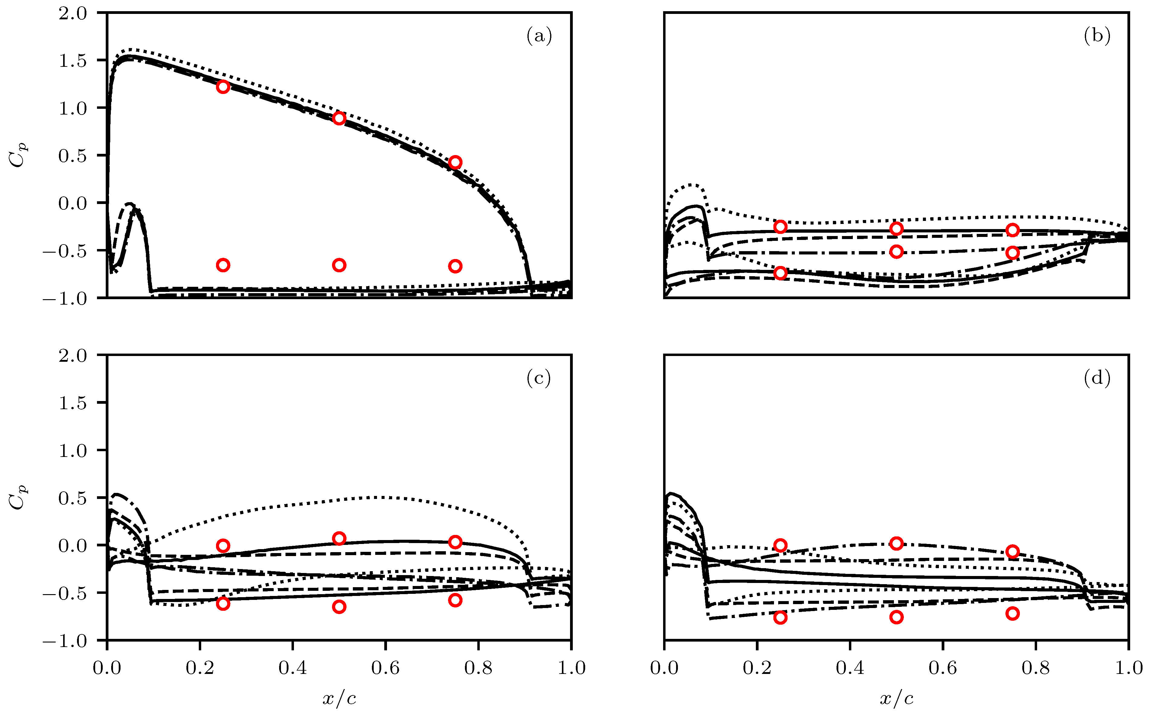
Pressure distributions obtained from the different simulations and the experimental measurements are reported in Figure 5 in terms of the pressure coefficient C p .
The pressure distributions on the 1st panel are shown in Figure 5a. All of the numerical results show the same pattern observed by the experimental measurements. Nevertheless, the RANS simulations tend to slightly overestimate the pressure difference between the front and the back side of the panel. This pressure difference is mostly due to a strong suction in the back side resulting from the acceleration of the flow below the 1st panel, which RANS simulations tend to overestimate.
For the 2nd panel, reported in Figure 5b, the three pressure-tap measurements of the back side show a constant pressure distribution, which is correctly reproduced by the numerical simulations. On the front side, measurements show that the pressure on the panel are not constant: the bottom corner has a lower pressure than in the backside of the previous panel; the rest of the panel, instead, has a slight recover in pressure. This behaviour is not reproduced by any of the simulations, which predict a constant pressure distribution in the front face of the 2nd panel. The measured pressure difference between the front and back sides at 0.25c is accurately reproduced by the k- ϵ , SST k- ω and RSM models, while the transition SST model fails in recovering it. On the contrary, for the points at 0.5c and 0.75c the transition SST model is the one to recover more accurately the measured pressure difference, while the other models show larger discrepancies. Both experiments and simulations shows lower pressure coefficient at the front side than at the back, which confirms that suction is occurring at the front side of the panel.
Figure 5c shows the results for the 3rd panel. It can be observed that the C p measurements match very well with the SST k- ω model, while the pressure difference between the front and back sides is slightly underestimated in the k- ϵ model. In any case, both the numerical simulations predict that the pressure is almost constant at each side of the panel; this behaviour is confirmed by the experimental measurements. The transition SST and RSM models, instead, shows a more diverse behavior, with the first predicting almost zero pressure difference and the latter predicting slightly higher pressure difference for x / c = 0.5 .
Results for the 4th panel are shown in Figure 5d. In this case, transition SST model reproduces more accurately than the other models the difference in pressure coefficients between the front and back side of the panel. Also on this panel the k- ϵ model slightly underestimates the pressure coefficient difference between the front and back sides of the panel. The SST k- ω and RSM models, instead, underestimate the pressure difference. Despite the differences in accuracy, all the turbulence models predict a constant pressure distribution along both the front and back sides of the panel, which is confirmed by the experimental measurements.

4.3. Turbulence Kinetic Energy k

Planar PIV measures only the in-plane velocity components ( u , v ) . The transversal velocity fluctuations of the flow are here neglected when compared with the ones in the tangential plane. The final value of the turbulence kinetic energy k is computed as:
k = 1 2 u 2 ¯ + v 2 ¯ ,
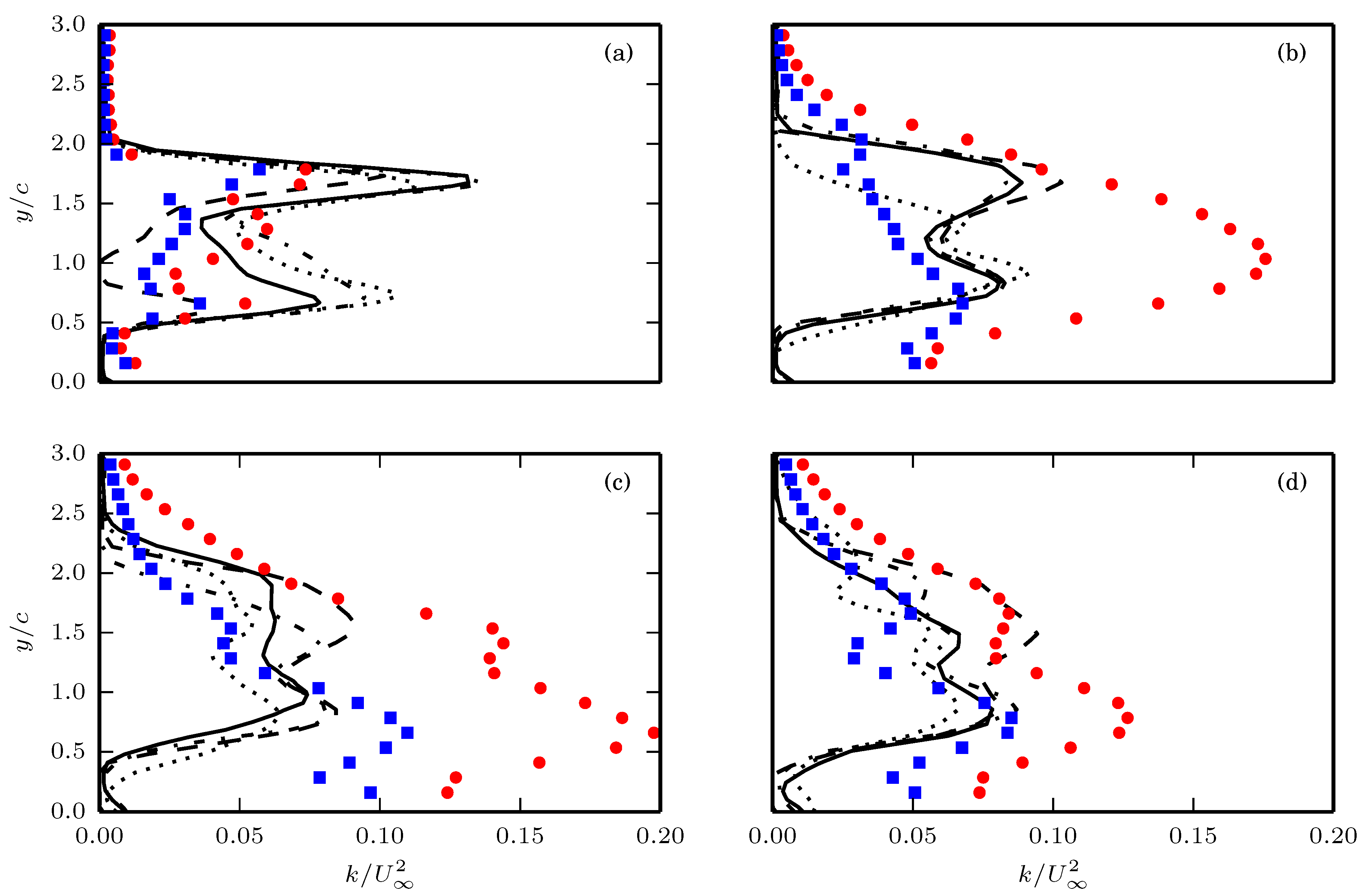
where u and v are the velocity fluctuations in the streamwise and vertical direction, respectively. Figure 6 shows the vertical profile of k between (a) 1st and 2nd panel ( x / c = 1.5 ), (b) 2nd and the 3rd panel ( x / c = 3.5 ), (c) 3rd and 4th panel ( x / c = 5.5 ), and (d) after the 4th panel ( x / c = 7.5 ). In addition, it is also shown the Reynolds stress u 2 ¯ .
In Figure 6a transition SST and SST k- ω models produces a k very similar to the measured Reynolds stress u 2 ¯ than to k, specially at y / c = 0.5 and 1.5, where the flow leaves the 1st panel at the bottom and top corners respectively. In this condition the flow is highly anisotropic, nevertheless due to the Boussinesq hypothesis k is often found to be in simulations larger than in experiments [40]. In any case, none of the numerical model fits perfectly with the experiment in the region inside the turbulent wake of the panel. It is remarkable that k- ϵ predicts no k at y / c = 1 , a region with a fully turbulent flow.
In Figure 6b the measured u 2 ¯ shows a more similar shape to the numerical k than the experimental one. k- ϵ , SST k- ω and transition SST predict the same k in the region inside the turbulent wake after the 2nd panel, while RSM prediction is slightly different from the other simulations. The RSM profile is more similar to the u 2 ¯ profile than the other methods, with a more intense fluctuation of the flow passing below the panels than of the one passing above. However, the numerical results are underestimated with respect to u 2 ¯ and k in this region. There is also difference between the measured u 2 ¯ and k in this region, which implies that the cross-wise fluctuations are strongly contributing to k. The region below the turbulent wake shows also a significant difference between the experimental and numerical k. The simulation predict that there is almost no k is this region. In the numerical fields for the mean horizontal velocity it was seen that, after the acceleration when leaving the 1st panel, the flow did not reduce its streamwise mean velocity as much as seen in the experiment. This could be possibly justified by the fact that no simulation is able to correctly predict the streamwise fluctuations of the flow passing below the panels, thus overestimating its momentum.
In Figure 6c the k predicted by k- ϵ is the most similar to the measured u 2 ¯ in the region above y / c = 1.5 . However, none of the numerical model gets to simulate neither k or u 2 ¯ in the turbulent wake after the 3rd panel. The region of larger k is thinner in the transition SST model than in the other three. This was expected behaviour after seen the thinner turbulent wake in the velocity fields of this model. The same difference in experimental and numerical k in the flow below the panels can be seen in this profile.
In Figure 6d the k predicted by k- ϵ is the most similar to the measured u 2 ¯ in the region above y / c = 1.5 . However, none of the numerical models gets to simulate neither k or u 2 ¯ in the turbulent wake after the 4th panel. In the region between y / c = 0.5 and y / c = 1.0 the numerical models clearly underestimate k. The same difference in experimental and numerical k in the flow below the panels can be seen in this profile.

5. Conclusions

The results of the RANS simulations with different solver models have been compared with experimental results for complex separated flows. These numerical methods are k- ϵ , SST k- ω , transitional SST and RSM. The experimental velocity and turbulent kinetic energy fields are investigated using PIV. Static pressure measurements are obtained by using pressure taps located on the surface model and a pressure transducer.
The average velocity fields obtained from the different numerical methods are in good agreement when compared with the experimental ones. However, there are some flow features that are not reproduced by all models, like the stretching in the turbulent wake between the 3rd and 4th panel. A good prediction of the velocity fields and the thickness of the turbulent wake is very important to rely on the loads produced by the numerical methods.
With respect to the pressure coefficients, the numerical models show different degrees of fidelity depending on the panel. All the numerical methods are reasonably good when simulating the pressure applied on the 1st panel due to the free flow impact, but they tend to overestimate the difference between the front and back sides. k- ϵ model tends to underestimate the pressure difference between the front and back sides. For the 3rd and 4th panel, k- ϵ tends to underestimate the pressure coefficient difference between the front and back sides, while SST k- ω provides a better estimation in the 3rd panel and transition SST in the 4th panel. In any case, all the numerical methods predicts correctly that the pressure is constant along the front and back sides when the flow is detached. In terms of the pressure coefficient difference between the front and back side of the panel, it seems that the methods that predicts better the thickness of the turbulent wake provides better results. k- ϵ and SST k- ω shows better behaviour that transition SST in this aspect.
The predicted k by the different numerical models is more similar to the experimental Reynolds stress u 2 ¯ than to the k. Most of the numerical methods analysed in this paper are based on the Boussinesq hypothesis, which implies that one of the Reynolds stresses is dominant over the other. For the complex separated flow in the experiment, it has been seen that both u 2 ¯ and v 2 ¯ are of the same order of magnitude, thus making the Boussinesq hypothesis invalid. However, also when removing this constrain, i.e., using the RSM model, the cross-wise fluctuations tend to be largely underestimated.
It can be concluded that after the flow separation in the 1st panel, the accuracy of the different numerical methods predicting the pressure on the panels does not depend so much on the robustness of the models as on fortune. On the other hand RSM seems to provide better estimations of the flow features, such as the wake shrink in the 3rd panel, as well as a better overall performances in estimating the pressure difference on the panels, which in most of the cases is more conservative than what measured. This advantage could rely on the fact that RSM is not based on the Boussinesq hypothesis, thus being more appropriate for this type of flows.
Nevertheless, it must be pointed out that our study has not coped all the RANS models available in literature. Additionally, the recent developments in numerical models and computational resources could take in a short time to better predictions of separated flows. One possibility could be, for example, the wavelet-based adaptive unsteady RANS model proposed by De Stefano et al. [41].

Author Contributions

Conceptualization, P.F. and M.R.; methodology, A.G., M.R. and P.F.; software, P.F.; investigation, A.G. and M.R.; formal analysis, A.G.; writing—original draft preparation, A.G.; writing—review and editing, M.R. and P.F. All authors have read and agreed to the published version of the manuscript.

Funding

This research received no external funding.

Acknowledgments

The authors wish to thanks Carlos Cobos for contributing the realisation of the experimental setup and J. Rodríguez for providing the PIV system. The authors acknowledge S. Discetti and A. Ianiro for insightful comments and discussions.

Conflicts of Interest

The authors declare no conflict of interest.

Nomenclature

cpanel-chord length
R e c chord Reynolds number
kturbulent kinetic energy
ϵ turbulent dissipation rate
ω specific turbulent dissipation rate
LESlarge-eddy simulation
PIVparticle image velocimetry
PODproper orthogonal decomposition
RANSReynolds-averaged Navier–Stokes
SSTshear stress transport
C p pressure coefficient

References

  1. ASCE. Minimum Design Loads for Buildings and Other Structures (ANSI/ASCE 7-93); American Society of Civil Engineers: Reston, VA, USA, 1994. [Google Scholar]
  2. Timilsina, G.R.; Kurdgelashvili, L.; Narbel, P.A. Solar energy: Markets, economics and policies. Renew. Sust. Energ. Rev. 2012, 16, 449–465. [Google Scholar] [CrossRef]
  3. Geyer, M.; Lüpfert, E.; Osuna, R.; Esteban, A.; Schiel, W.; Schweitzer, A.; Zarza, E.; Nava, P.; Langenkamp, J.; Mandelberg, E. EUROTROUGH-Parabolic trough collector developed for cost efficient solar power generation. In Proceedings of the 11th International Symposium on Concentrating Solar Power and Chemical Energy Technologies, Zurich, Switzerland, 4–6 September 2002. [Google Scholar]
  4. Karin, T.; Jones, C.B.; Jain, A. Photovoltaic Degradation Climate Zones. In Proceedings of the IEEE 46th Photovoltaic Specialists Conference, Chicago, IL, USA, 16–21 June 2019; pp. 687–694. [Google Scholar]
  5. Dunlop, E.D.; Halton, D. The performance of crystalline silicon photovoltaic solar modules after 22 years of continuous outdoor exposure. Prog. Photovoltaics 2006, 14, 53–64. [Google Scholar] [CrossRef]
  6. Skoczek, A.; Sample, T.; Dunlop, E.D. The results of performance measurements of field-aged crystalline silicon photovoltaic modules. Prog. Photovoltaics 2009, 17, 227–240. [Google Scholar] [CrossRef]
  7. Poulek, V.; Šafránková, J.; Černá, L.; Libra, M.; Beránek, V.; Finsterle, T.; Hrzina, P. PV Panel and PV Inverter Damages Caused by Combination of Edge Delamination, Water Penetration, and High String Voltage in Moderate Climate. IEEE J. Photovolt. 2021. [Google Scholar] [CrossRef]
  8. Stenabaugh, S.E.; Iida, Y.; Kopp, G.A.; Karava, P. Wind loads on photovoltaic arrays mounted parallel to sloped roofs on low-rise buildings. J. Wind Eng. Ind. Aerod. 2015, 139, 16–26. [Google Scholar] [CrossRef]
  9. Naeiji, A.; Raji, F.; Zisis, I. Wind loads on residential scale rooftop photovoltaic panels. J. Wind Eng. Ind. Aerod. 2017, 168, 228–246. [Google Scholar] [CrossRef]
  10. Chu, C.R.; Tsao, S.J. Aerodynamic loading of solar trackers on flat-roofed buildings. J. Wind Eng. Ind. Aerod. 2018, 175, 202–212. [Google Scholar] [CrossRef]
  11. Wang, J.; Yang, Q.; Tamura, Y. Effects of building parameters on wind loads on flat-roof-mounted solar arrays. J. Wind Eng. Ind. Aerod. 2018, 174, 210–224. [Google Scholar] [CrossRef]
  12. Bitsuamlak, G.T.; Dagnew, A.K.; Erwin, J. Evaluation of wind loads on solar panel modules using CFD. In Proceedings of the Fifth International Symposium on Computational Wind Engineering, Chapel Hill, NC, USA, 23–27 May 2010. [Google Scholar]
  13. Shademan, M.; Hangan, H. Wind loading on solar panels at different azimuthal and inclination angles. In Proceedings of the Fifth International Symposium on Computational Wind Engineering, Chapel Hill, NC, USA, 23–27 May 2010. [Google Scholar]
  14. Shademan, M.; Barron, R.; Balachandar, R.; Hangan, H. Numerical simulation of wind loading on ground-mounted solar panels at different flow configurations. Can. J. Civ. Eng. 2014, 41, 728–738. [Google Scholar] [CrossRef]
  15. Jubayer, C.M.; Hangan, H. A numerical approach to the investigation of wind loading on an array of ground mounted solar photovoltaic (PV) panels. J. Wind Eng. Ind. Aerod. 2016, 153, 60–70. [Google Scholar] [CrossRef]
  16. Reina, G.P.; De Stefano, G. Computational evaluation of wind loads on sun-tracking ground-mounted photovoltaic panel arrays. J. Wind Eng. Ind. Aerod. 2017, 170, 283–293. [Google Scholar] [CrossRef]
  17. Chevalier, H.; Norton, D. Wind Loads on Solar Collector Panels and Support Structure; Technical report; Department of Aerospace Engineering, Texas A&M University: College Station, TX, USA, 1979. [Google Scholar]
  18. Abiola-Ogedengbe, A.; Hangan, H.; Siddiqui, K. Experimental investigation of wind effects on a standalone photovoltaic (PV) module. Renew. Energy 2015, 78, 657–665. [Google Scholar] [CrossRef]
  19. García, E.T.; Ogueta-Gutiérrez, M.; Ávila, S.; Franchini, S.; Herrera, E.; Meseguer, J. On the effects of windbreaks on the aerodynamic loads over parabolic solar troughs. Appl. Energ. 2014, 115, 293–300. [Google Scholar] [CrossRef] [Green Version]
  20. Etyemezian, V.; Nikolich, G.; Gillies, J. Mean flow through utility scale solar facilities and preliminary insights on dust impacts. J. Wind Eng. Ind. Aerod. 2017, 162, 45–56. [Google Scholar] [CrossRef] [Green Version]
  21. Bush, R.H.; Chyczewski, T.S.; Duraisamy, K.; Eisfeld, B.; Rumsey, C.L.; Smith, B.R. Recommendations for future efforts in rans modeling and simulation. In Proceedings of the AIAA Scitech 2019 Forum, San Diego, CA, USA, 7–11 January 2019; p. 317. [Google Scholar]
  22. Menter, F.R. Zonal two equation k-ω turbulence models for aerodynamic flows. In Proceedings of the 23rd Fluid Dynamics, Plasmadynamics, and Lasers Conference, Orlando, FL, USA, 6–9 July 1993; p. 2906. [Google Scholar]
  23. Menter, F.R. Two-equation eddy-viscosity turbulence models for engineering applications. AIAA J. 1994, 32, 1598–1605. [Google Scholar] [CrossRef] [Green Version]
  24. Menter, F.; Kuntz, M.; Langtry, R. Ten years of industrial experience with the SST turbulence model. Turbul. Heat Mass Transf. 2003, 4, 625–632. [Google Scholar]
  25. Blocken, B.; van der Hout, A.; Dekker, J.; Weiler, O. CFD simulation of wind flow over natural complex terrain: Case study with validation by field measurements for Ria de Ferrol, Galicia, Spain. J. Wind Eng. Ind. Aerod. 2015, 147, 43–57. [Google Scholar] [CrossRef]
  26. Catalano, P.; Wang, M.; Iaccarino, G.; Moin, P. Numerical simulation of the flow around a circular cylinder at high Reynolds numbers. Int. J. Heat Fluid Flow 2003, 24, 463–469. [Google Scholar] [CrossRef]
  27. Mendez, M.; Raiola, M.; Masullo, A.; Discetti, S.; Ianiro, A.; Theunissen, R.; Buchlin, J.M. POD-based background removal for particle image velocimetry. Exp. Therm. Fluid Sci. 2017, 80, 181–192. [Google Scholar] [CrossRef] [Green Version]
  28. Astarita, T.; Cardone, G. Analysis of interpolation schemes for image deformation methods in PIV. Exp. Fluids 2005, 38, 233–243. [Google Scholar] [CrossRef]
  29. Astarita, T. Analysis of weighting windows for image deformation methods in PIV. Exp. Fluids 2007, 43, 859–872. [Google Scholar] [CrossRef]
  30. Westerweel, J.; Scarano, F. Universal outlier detection for PIV data. Exp. Fluids 2005, 39, 1096–1100. [Google Scholar] [CrossRef]
  31. Westerweel, J. Fundamentals of digital particle image velocimetry. Meas. Sci. Technol. 1997, 8, 1379. [Google Scholar] [CrossRef] [Green Version]
  32. Launder, B.E.; Spalding, D.B. The numerical computation of turbulent flows. Comput. Methods Appl. Mech. Eng. 2014, 3, 269–289. [Google Scholar] [CrossRef]
  33. Galindo, J.; Hoyas, S.; Fajardo, P.; Navarro, R. Set-up analysis and optimization of CFD simulations for radial turbines. Eng. Appl. Comput. Fluid Mech. 2013, 7, 441–460. [Google Scholar] [CrossRef] [Green Version]
  34. Wilcox, D.C. Reassessment of the scale-determining equation for advanced turbulence models. AIAA J. 1988, 26, 1299–1310. [Google Scholar] [CrossRef]
  35. Menter, F.R.; Langtry, R.; Likki, S.; Suzen, Y.; Huang, P.; Völker, S. A correlation-based transition model using local variables—Part I: Model formulation. J. Turbomach. 2006, 128, 413–422. [Google Scholar] [CrossRef]
  36. Craft, T.; Launder, B.; Suga, K. Development and application of a cubic eddy-viscosity model of turbulence. Int. J. Heat Fluid Fl. 1996, 17, 108–115. [Google Scholar] [CrossRef]
  37. Launder, B.E.; Reece, G.J.; Rodi, W. Progress in the development of a Reynolds-stress turbulence closure. J. Fluid Mech. 1975, 68, 537–566. [Google Scholar] [CrossRef] [Green Version]
  38. Chou, P.Y. On velocity correlations and the solutions of the equations of turbulent fluctuation. Q. Appl. Math. 1945, 3, 38–54. [Google Scholar] [CrossRef] [Green Version]
  39. Rotta, J. Statistische theorie nichthomogener turbulenz. Z. Phys. 1951, 129, 547–572. [Google Scholar] [CrossRef]
  40. Durbin, P. On the k-ε stagnation point anomaly. Int. J. Heat Fluid Flow 1996, 17, 9–90. [Google Scholar] [CrossRef]
  41. De Stefano, G.; Vasilyev, O.V.; Brown-Dymkoski, E. Wavelet-based adaptive unsteady Reynolds-averaged turbulence modelling of external flows. J. Fluid Mech. 2018, 837, 765–787. [Google Scholar] [CrossRef]
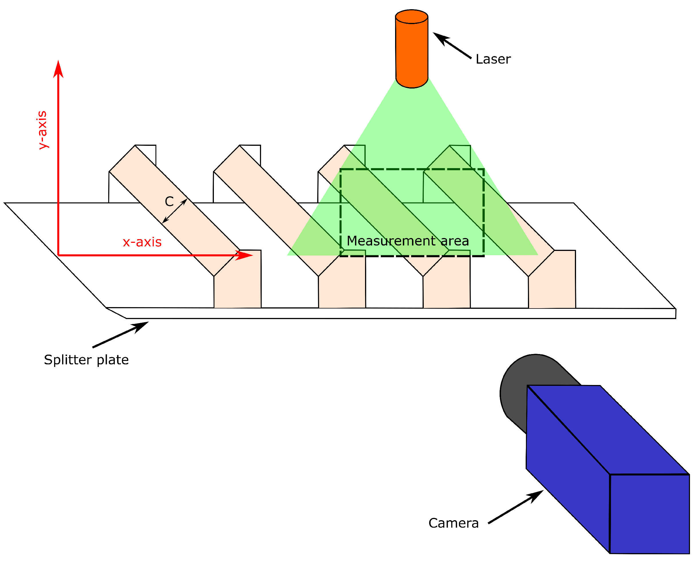
Figure 1. Sketch of the experimental setup. The streamwise and vertical direction are indicated as x and y, respectively.
Applsci 11 02496 g001
Figure 2. Schematic of the pressure taps on panel.
Applsci 11 02496 g002
Figure 3. Computational domain.
Applsci 11 02496 g003
Figure 4. Contour map of the average horizontal (left column) and vertical (right column) velocity components. From top to bottom, rows refer to experimental measurements, transitional SST, k- ω SST, k- ϵ and RSM. The horizontal and vertical dimensions are normalised with respect to the panel chord length c. The velocity magnitude is normalised with respect to the inlet free-stream velocity measured in the wind tunnel. Solar panels are shown in black color. For experimental measurements, areas below the solar panels in which the laser illumination was not sufficient are blanked in white color.
Applsci 11 02496 g004
Figure 5. Pressure coefficient C p distribution for (a) 1st panel, (b) 2nd panel, (c) 3rd panel, and (d) 4th panel. Lines refers to numerical results for the different turbulent models: k- ϵ ( Applsci 11 02496 i001); SST k- ω ( Applsci 11 02496 i002); transition SST ( Applsci 11 02496 i003); and RSM (▪▪▪▪▪▪▪). Experimental measurements are shown as ().
Applsci 11 02496 g005
Figure 6. Turbulent kinetic energy k profiles at (a) x / c = 1.5 , (b) x / c = 3.5 , (c) x / c = 5.5 , and (d) x / c = 7.5 . Lines refers to numerical results for the different turbulent models: k- ϵ ( Applsci 11 02496 i001); SST k- ω ( Applsci 11 02496 i002); transition SST ( Applsci 11 02496 i003); and RSM (▪▪▪▪▪▪▪). Experimental k is shown as (), while u 2 ¯ is referred as (). The vertical dimension is normalised with respect to the panel chord length c. The energy magnitude is normalised with respect to the power square of the inlet free-stream velocity measured in the wind tunnel.
Applsci 11 02496 g006
Publisher’s Note: MDPI stays neutral with regard to jurisdictional claims in published maps and institutional affiliations.