Article

Time Series Clustering of Online Gambling Activities for Addicted Users’ Detection

1
Nova Information Management School (NOVA IMS), Universidade NOVA de Lisboa, Campus de Campolide, 1070-312 Lisboa, Portugal
2
Dipartimento di Matematica e Geoscienze, Università degli Studi di Trieste, Via Valerio 12/1, 34127 Trieste, Italy
3
Faculty of Economics, University of Ljubljana. Kardeljeva Ploščad 17, 1000 Ljubljana, Slovenia
4
SRIJ, Serviço de Regulação e Inspeção de Jogos, Rua Ivone Silva, 1050-124 Lisboa, Portugal
*
Author to whom correspondence should be addressed.
Appl. Sci. 2021, 11(5), 2397; https://doi.org/10.3390/app11052397
Submission received: 2 February 2021 / Revised: 22 February 2021 / Accepted: 24 February 2021 / Published: 8 March 2021
(This article belongs to the Section Computing and Artificial Intelligence)

Abstract

:
Ever since the worldwide demand for gambling services started to spread, its expansion has continued steadily. To wit, online gambling is a major industry in every European country, generating billions of Euros in revenue for commercial actors and governments alike. Despite such evidently beneficial effects, online gambling is ultimately a vast social experiment with potentially disastrous social and personal consequences that could result in an overall deterioration of social and familial relationships. Despite the relevance of this problem in society, there is a lack of tools for characterizing the behavior of online gamblers based on the data that are collected daily by betting platforms. This paper uses a time series clustering algorithm that can help decision-makers in identifying behaviors associated with potential pathological gamblers. In particular, experimental results obtained by analyzing sports event bets and black jack data demonstrate the suitability of the proposed method in detecting critical (i.e., pathological) players. This algorithm is the first component of a system developed in collaboration with the Portuguese authority for the control of betting activities.

1. Introduction

Ever since the worldwide demand for gambling services started to spread, its expansion has continued steadily. The main factor contributing to this ongoing expansion is the explosion of telecommunication technologies that have facilitated the development of new gaming services, along with a wide variety of new delivery channels for gambling services [1].
According to the European Gaming and Betting Association, Europe currently represents the largest international market for online gambling, with a Gross Gaming Revenue (GGR) expected to reach 24.9 billion Euros by the end of 2020 [2]. To wit, online gambling is a major industry in every European country, generating billions of Euros in revenue for commercial actors and governments alike. Despite such evidently beneficial effects, online gambling is ultimately a vast social experiment with potentially disastrous social and personal consequences that could result in an overall deterioration of social and familial relationships [3].
A recent study [4] examined the issues associated with problem gambling and indicators of mental and physical health, as well as psychosocial adjustment and health care usage, in a representative sample of online gamblers. The results show significant correlations among problem gambling and mental health issues (anxiety, neurotic symptoms, and substance abuse) and psychosocial maladjustment (suicidality, financial difficulties, and reduced social support). These findings reinforce the reality of that addiction as a public health concern. Another study [5] analyzed the financial, productivity-related, personal, and family costs associated with online gambling; it showed that these costs are generally greater than gambling taxation income. This is to say that a gambling addiction tends to have a detrimental effect on public finances.
In 2012, the European Commission released a statement [1] highlighting the need for regulatory policies to aid in the detection of pathological gambling behaviors, citing “a responsibility to protect those citizens and families who suffer from a gambling addiction.” Despite this earnest recommendation, research aimed at developing a coherent set of responsible national policies has yet to make it past the embryonic stage. In Portugal, the Gambling Inspection and Regulation Service is “responsible for the control and regulation of gambling activities in casinos and bingo halls, as well as online gambling and betting.” To comply with operational and regulatory objectives, this authority receives, on a daily basis, all data related to online gambling activities pursued by every user on every online platform with services that are accessible to Portuguese citizens. In spite of this prodigious collection of data, the authority still lacks appropriate tools for identifying gambling addicts. This authority acknowledges a profound scarcity of actionable data regarding the actual scope of gambling addiction and a consequent lack of expertise about how best to deal with this problem. The same authority observes that “the human dimension and economical and social relevance of this issue (i.e., gambling addiction) demands scientific studies.”
To answer this call, this paper proposes an ML (Machine Learning)-based tool that could capitalize on the vast amount of data collected every day and analyze online user behavior to model and detect the behaviors associated with addicted gamblers. The problem represents a major challenge due the massive amount of data involved.
To tackle this problem, we use a clustering algorithm specifically developed for time series, namely dynamic time warping, and we show its suitability in identifying different subsets of gamblers that are characterized by a specific behavior. In particular, DTW can identify a subset of gamblers characterized by uncommon behaviors (i.e., a significant amount of money spent, number of accesses to the gambling provider platforms, etc.), thus simplifying the subsequent work of the gambling authority. We envision this as the first step towards an AI (Artificial Intelligence)-based system that is able to constantly assess gamblers’ behavior and to raise an alert every time a user is perceived as an addicted gambler.
This study is fully supported by the Gambling Inspection and Regulation Service of Portugal (SRIJ (Serviço de Regulação e Inspeção de Jogos)), the national authority for the control, inspection, and regulation of gambling activities. The AI-based system implemented will be integrated into the SRIJ infrastructure, thereby providing a working solution to the problem of the lack of protection and control currently applied to users. In this way, the authority could deploy all actions it regards as necessary to help addicted players. The social impact would be enormous, given its inherent capacity to reduce the social costs associated with gambling addiction.
The remaining part of the paper is organized as follows: Section 2 presents a literature review in the area of pathological gambling detection; Appendix A presents all the details of the clustering technique used in this paper, by describing important concepts on time series analysis; Section 3 describes the experimental settings, while Section 4 discusses the results achieved. Finally, Section 5 concludes the paper and suggests future research directions.

2. Literature Review

In response to the proliferation of online gambling services, the scientific literature has proposed the use of AI-based techniques to analyze this phenomenon. Broadly speaking, two primary strands of research are identifiable in the literature. The first of these threads aims to understand the behavior of gamblers, to undertake business policies capable of effectively retaining them as consumers. To that end, churn prediction has proven to be a promising tactical option within the context of the Customer Relationship Management (CRM) strategy for analyzing the dynamics and dimensions of customer retention. In this context, it refers to the process of identifying gamblers with a high probability of leaving the company, on the basis of past behavior. For instance, Reference [6] investigated whether churn prediction is a valuable option to include in the CRM palette of online gambling companies. Using real-life data provided by an online gambling company, a combination of single algorithms, CART decision trees, and generalized additive models is benchmarked to their ensemble counterparts. The results reflect the strategic value of churn prediction for identifying and profiling those customers that, with a high degree of probability, might leave the gambling provider, consequently causing a loss of revenue.
The second strand of research aims to study the characteristic behaviors of so-called gambling addicts. The ability to identify gamblers whose behavior resembles that of gamblers who elected to use self-exclusion tools or were identified as problematic gamblers by other online platforms could, for instance, be used to target responsible gaming messages to amplify self-awareness among gamblers, thereby reducing the risk of adverse outcomes [7]. Depending on the availability of transactional gambling data, most research aimed at identifying the predictors for gambling-related problems focuses on daily aggregates of gambling transactions from business-to-customer gambling operations [8].
In spite of the burgeoning interest in this area, the vast majority of existing studies do not use AI-based techniques to aid in the detection of addicted gamblers; instead, they rely on simple statistical techniques to accomplish the same objectives. In a recent study [8], the authors examined all peer-reviewed empirical evidence underpinning the pursuit of Responsible Gambling (RG) strategies. The results show that current evidence about RG initiatives and programs is very limited. The authors observed the nascent state of the field, which has not yet progressed to best practices that are supported by scientific evidence, and further, to the fact that RG programs that rely on AI tools remain largely at the nascent stage of development.
A recent contribution to the literature [9] used Artificial Neural Networks (ANNs) to investigate the extent to which specific payment behaviors and methods facilitate accurate identification of problematic gamblers; the point of origin for the study is the transactional data generated by customers of the online gambling provider bwin.com. The resulting ANN is quite naive and incapable of capturing the intrinsic temporal dimension of the data. Likewise, the authors of [10] evaluated a set of classification and regression algorithms to determine which techniques are more qualified to identify probable addicted gamblers. According to this study, while ANNs are evidently the most reliable classification method overall, they still fail to identify a meaningfully large group of likely problem gamblers. Such studies indicate that the use of AI techniques to detect gambling addicts is still in its infancy. Scientific literature [11] has pointed out that, to understand gambling behavior, it is essential to examine the behavioral patterns of play; there is good evidence to suggest that past behaviors can be used to predict future gambling actions and potential problems. Moreover, according to a recent study [12], personalized feedback about actual gambling behavior, generated by tracking player behavior, should have greater utility for informed player choice than generic information about best practices (e.g., adherence to a pre-set monetary limit). Following this idea, Gustafson [13] proposed using decision trees to identify potential addicted gamblers by using behavioral features like the time spent gambling, the rate of won and lost money, and the number of deposits made. The effect of modifying the monetary limit was investigated with ML techniques by Auer and Griffiths [14]. The authors used random forest and gradient boost algorithms to predict future limit-setting based on player behavior. They identified a set of variables that can predict the future limit-setting personal monthly loss limit, the amount bet, theoretical loss, and whether the players had increased their limits in the past.
An examination of the available literature underscores the need for more advanced tools to analyze the vast amount of behavioral data to promote much-needed advances in the RG field.
This paper answers this call-to-action by proposing an ML-based system that relies on a simple clustering algorithm. Specifically, the system will analyze historical data to extract behavioral clusters associated with potential pathological gamblers. To the best of our knowledge, this will be the first real-time system used by a public entity to analyze behavioral data associated with online gambling activities and collected by the different gambling providers themselves.

3. Experimental Phase

This section describes the data used in the experimental phase, as well as the considered experimental setting.
Data were provided by the Gambling Inspection and Regulation Service of Portugal after removing all personal information (i.e., name, surname, taxpayer number, address). Due to the existing regulation, data cannot be made available. To identify different users’ profiles that may allow discovering high-risk pathological gamblers, we relied on a K-means algorithm based on the dynamic time warping algorithm [15,16,17], a well-known technique that makes it possible to align and compare time series. For an introduction to time series analysis and a complete description of the dynamic time warping algorithm, the reader is referred to the material in the Appendix.

3.1. Data

Data used in the experimental phase came from ten different online gambling operators, each of which provides two monthly data sets containing sports and black jack bets’ data, respectively. The data sets must follow specific rules regarding the type and format of the data to be stored. For each bet played, the following variables are available:
  • player_id: unique identifier of the player in the operator system.
  • player_logon: username of the player in the operator system.
  • cod_ficha: unique identifier for a bet.
  • cod_ficha_jog: gambling external code attributed by the online gambling operator.
  • cod_aptr_jog: betting code used by the online gambling operator.
  • timestp_ini: start time of betting event.
  • timestp_fim: end time of betting event.
  • timestp: timestamp of the betting operation placed by a user.
  • a_saldo_ini: balance before the betting start.
  • a_valor: value of the bet.
  • a_saldo_fim: balance after betting close.
  • a_bonus_ini: player bonus before betting start.
  • a_bonus: bet bonus.
  • a_bonus_fim: player bonus after betting close.
  • g_ganho: amount won from the bet.
The data preparation phase aims at obtaining two different data sets, one for each type of game involved, that contain the time series of users’ bets. For this purpose, this phase consists of three steps: aggregation, concatenation, and time series creation. The last two phases are identical for both the considered games, while the aggregation phase differs between sports betting and black jack.
Before looking at each of these three phases in detail, it is necessary to clarify the following: a time series of bets for a single user cannot be given by the sequence of the g_ganho of his/her placed bets, as these values represent the amounts won from the bets, but not those lost. Thus, they are not suitable for fully representing the players’ behavior. To overcome this issue, the values composing the time series are obtained as the difference between the eventual g_ganho and the a_valor. In this way, each point of a given time series represents the final balance of a single bet, which can be positive, zero, or negative. More formally, we have:
  • N: number of gamblers.
  • n i : number of bets placed by the player i { 0 , , N } .
  • T i = { t 0 , , t n i } 
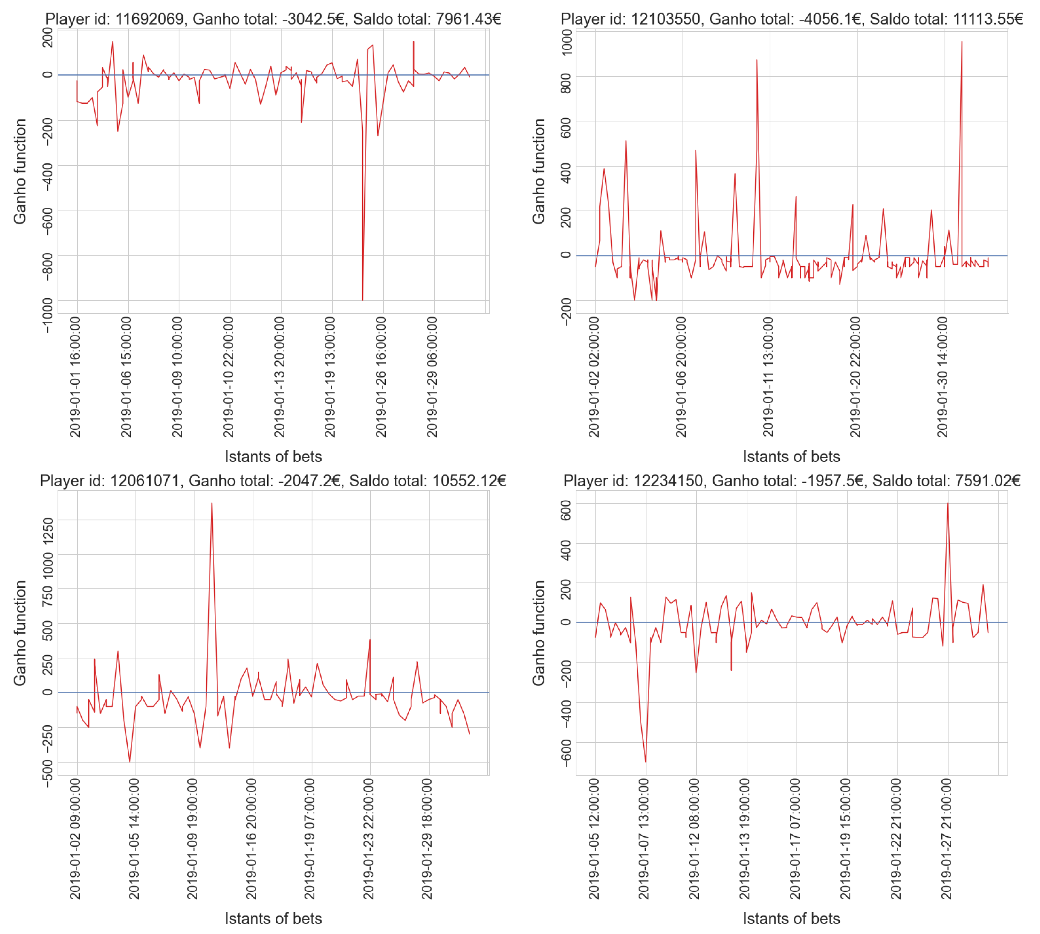
instants of bets for player i.
  • x t i = g _ ganho ( t i ) a _ valor ( t i ) balance of the bet placed in t i T i .
By doing this, we obtain a set of time series X = { x 0 , , x N } , where x i = ( x t 0 , , x t n i ) i { 0 , , N } .
The aggregation phase aims at reducing the size of the initial data set by extracting relevant information used to create the time series data set. Given a raw data set, this procedure returns a table of nine columns in which a single row represents a bet, for which the following information is stored:
  • player_id
  • player_logon
  • cod_ficha
  • cod_ficha_jog
  • cod_aptr_jog
  • timestp: the instant of the bet.
  • a_valor: value of the bet, including bonuses.
  • g_ganho: balance of the bet.
g_ganho now represents the the final balance of a single bet, obtained as described before. Moreover, a_valor is stored to know the amount of money placed on a specific bet. This phase is different for black jack and sports bets. In the former case, each bet corresponds exactly to a single row, given the nature of this game in which a player knows immediately the outcome of a single hand. Concerning sports bets, a single bet can generate different rows in the raw data set because; even if the bet is already placed by a player, the odds can change. Thus, an intermediate step in which the value and the final balance of the bet is taken from the most recent line of the same bet (not considering the others) is needed.
The concatenation phase has the goal of taking the aggregated data sets by type of game and joining them to obtain a single data set containing all the bets related to the considered game. This procedure also sorts the bets based on player_id and timestp, ensuring that in the next phase, the bets are ready to be grouped into the corresponding time series. This phase is pretty simple, but it is very useful as it allows performing the subsequent phase of the time series creation in a simple and efficient way.
The last phase of data preparation is the time series creation phase. In this phase, by using the concatenated data set, the time series of bets are created. This is done by grouping all the bets of a single player according to player_id. Not all the time series of the players are inserted into the final data set: some are discarded based on the number of bets they contain. This is reasonable given the nature of our problem. In particular, below a reasonable number of bets, a player cannot certainly be considered pathological. This threshold obviously varies according to the game considered. In the experimental phase, we considered the following monthly threshold values: five sports bets and thirty hands for black jack. All time series that have fewer plays than the game they refer to are removed. In the final data set, for each time series, the aggregated values for the balance and value of bets are also stored, to obtain two aggregate indicators of the gambler in the considered period.
All in all, the columns that form the final data set are:
  • player_id
  • time_stamp: sequence of timestp in which the bets are placed.
  • player_logon
  • cod_ficha: sequence of cod_ficha, useful to identify the single bets.
  • cod_aptr_jog sequence of cod_aptr_jog.
  • cod_fichajog: sequence of cod_fichajog.
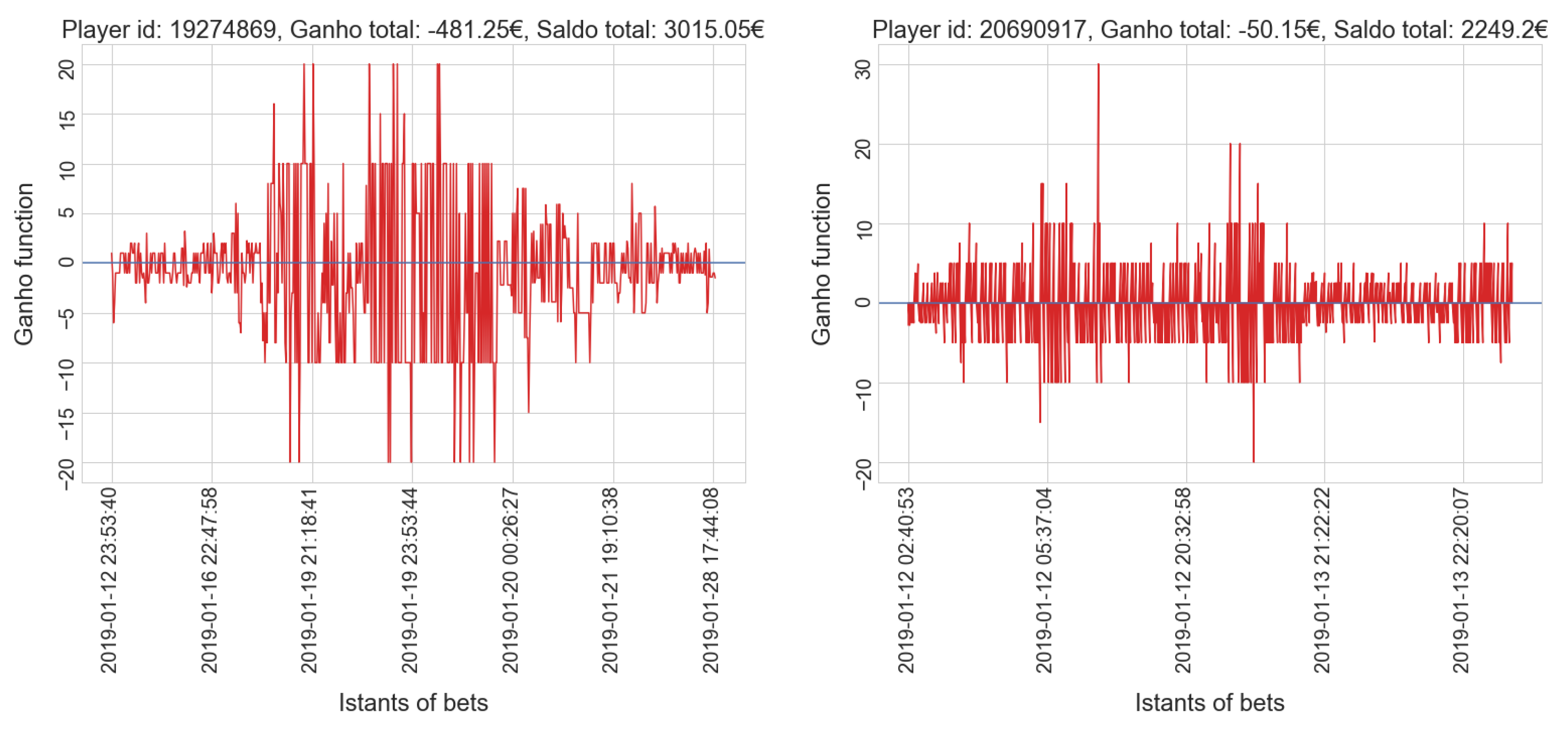
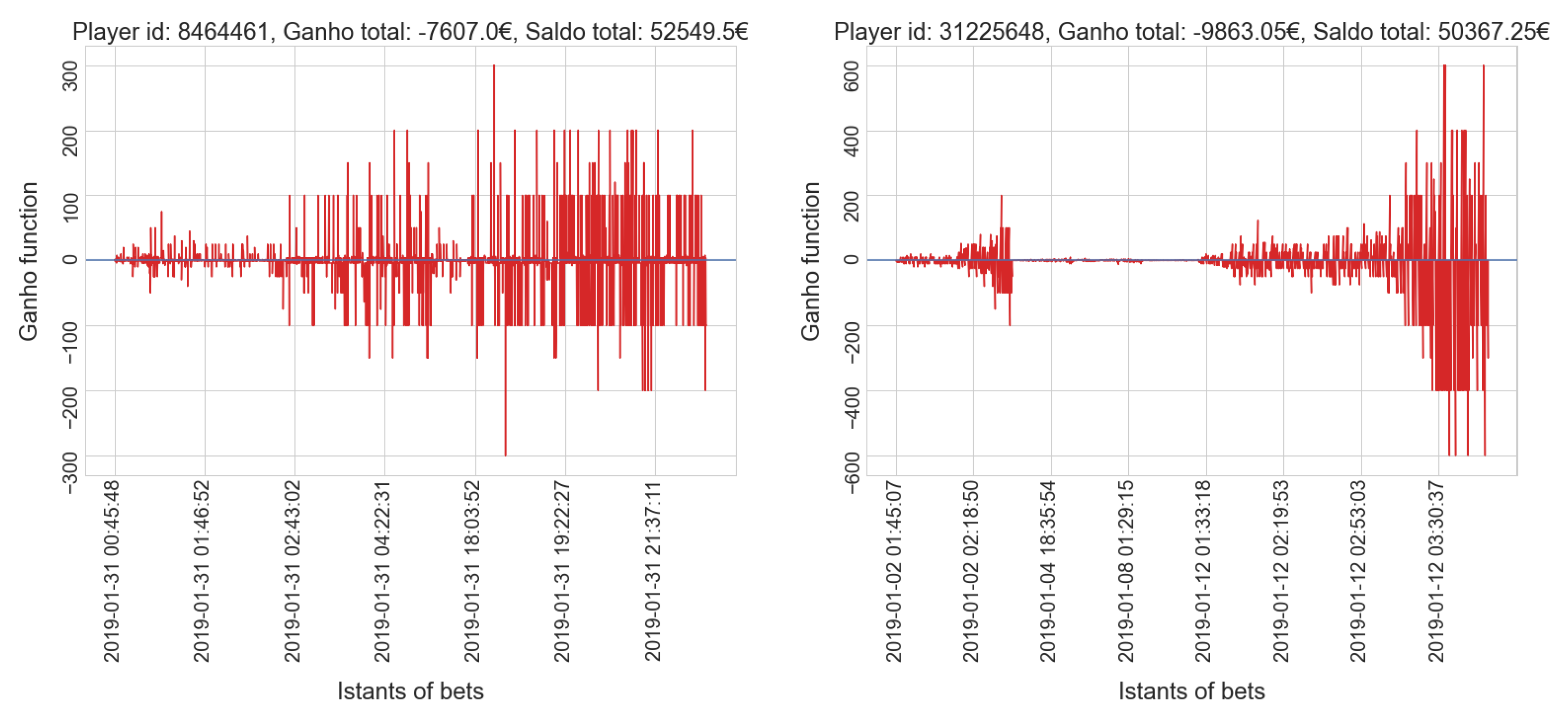
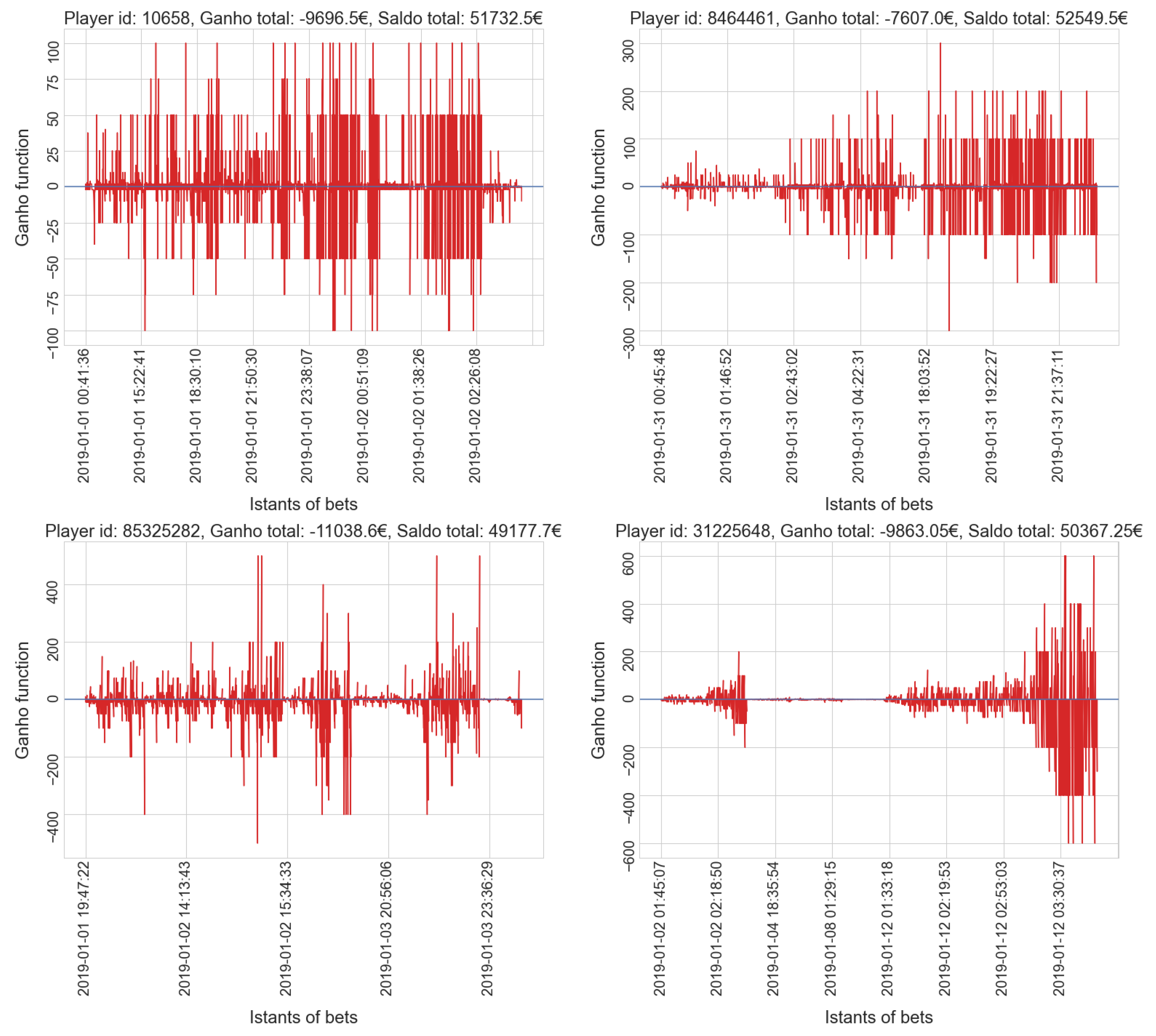
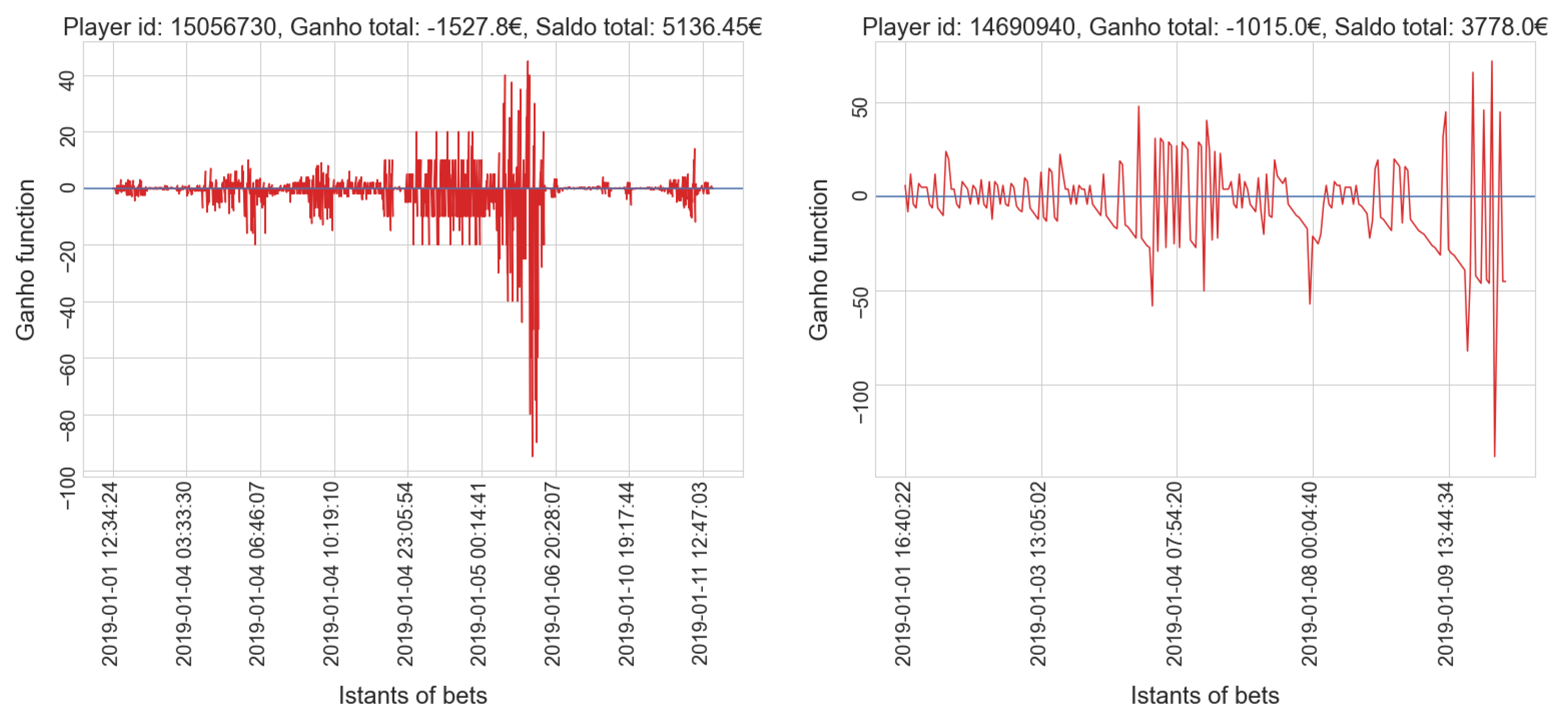
  • g_ganho: time series of the balances of player’s bets.
  • a_valor: sequence of a_valor.
  • g_ganho_tot: sum of the balances of the player.
  • a_saldo_tot: sum of the bets’ value of the player.
It is important to point out that the SRIJ data used in this study were anonymized, thus not allowing the identification of any player.
Table 1 shows, for the two types of games, the number of raw data sets, their total size, the size of the final data set, and the number of time series contained in it. All time series represent one month of bets. The final number of time series excludes the time series with fewer than five bets (for sports) or thirty hands (for black jack).

3.2. Experimental Settings

The clustering allows performing time series K-means on the data sets obtained from the data preparation phase. The optimal value of k, the number of clusters to form, can be obtained using the elbow method. The silhouette score is also used to assess the consistency of the results given by the elbow method.
The strategy used to obtain the results was the following: the elbow method was used, with k ranging from two to eight, to obtain an indication regarding the optimal number of clusters to create; subsequently, the silhouette score was calculated using the possible optimal values of k indicated by the previous method, aiming at assessing the consistency of the previous results and providing a further indication about the ideal value of k. After that, the clustering algorithm was performed with the chosen k.
The experimental phase was performed on the Galileo supercomputer. Galileo has currently 102,236 core compute nodes. Each one contains 218 core Intel Xeon E5-2697 v4 (Broadwell) at 2.30 GHz. All the compute nodes have 128 GB of memory. In more detail, this supercomputer has the following technical specifications:
  • Model: Lenovo NeXtScale
  • Architecture: Linux Infiniband Cluster
  • Nodes: 1022
  • Processors: 2 × 18-cores Intel Xeon E5-2697 v4 (Broadwell) at 2.30 GHz
  • Cores: 36 cores/node
  • RAM: 128 GB/node, 3.5 GB/core
  • Internal Network: Intel OmniPath, 100 Gb/s
  • Peak performance single node: 1.3 TFlop/s
  • Peak Performance: 1.5 PFlop/s
  • Accelerators: 60 nodes equipped with 1 Nvidia K80 GPU and 2 nodes equipped with 1 Nvidia V100 GPU
We relied on the implementation of time series k-means available in the tslearn Python package. However, we had to modify some parts of the library source code due to the following two reasons:
  • multiple calls to a data preparation function.
  • part of the computation of the algorithm does not take place in parallel.
The first problem was encountered during the first application of the algorithm: the calculation of the distance matrices was interrupted after a few minutes of computation due to a memory error. We found that this type of error was caused by multiple calls to the function to_time_series_data set(·) that transforms a time series data set so that it fits the format used in tslearn models. This function was called at each iteration of the k-means algorithm and also at each iteration of the barycenter computation process, causing memory and performance problems. This issue was addressed by eliminating redundant calls to this function and keeping only the first. After solving this problem, we realized that the algorithm continued to have a very high execution time, and we discovered that only the computation of the distance matrices (DTW) actually took place in parallel, while the DTW Barycenter Averaging (DBA) part took place in serial. To solve this problem, it was decided to completely rewrite the code related to the DBA part, with the aim of making it efficient, in terms of memory and computational time. The dynamic barycenter averaging procedure is mainly composed of three different functions:
  • _mm_assignment: computes item assignment based on DTW alignments and returns cost as a bonus.
  • _mm_valence_warping: computes valence and warping matrices from paths, returning the sum of diagonals and a list of matrices.
  • _mm_update_barycenter: updates the barycenters.
All three functions were rewritten in parallel, allowing us to perform the DBA procedure in the following way: for each cluster, a process that spawns a pool of threads used to perform the dynamic barycenter averaging procedure is created. Therefore, this procedure is performed simultaneously for all the clusters.

4. Results and Discussion
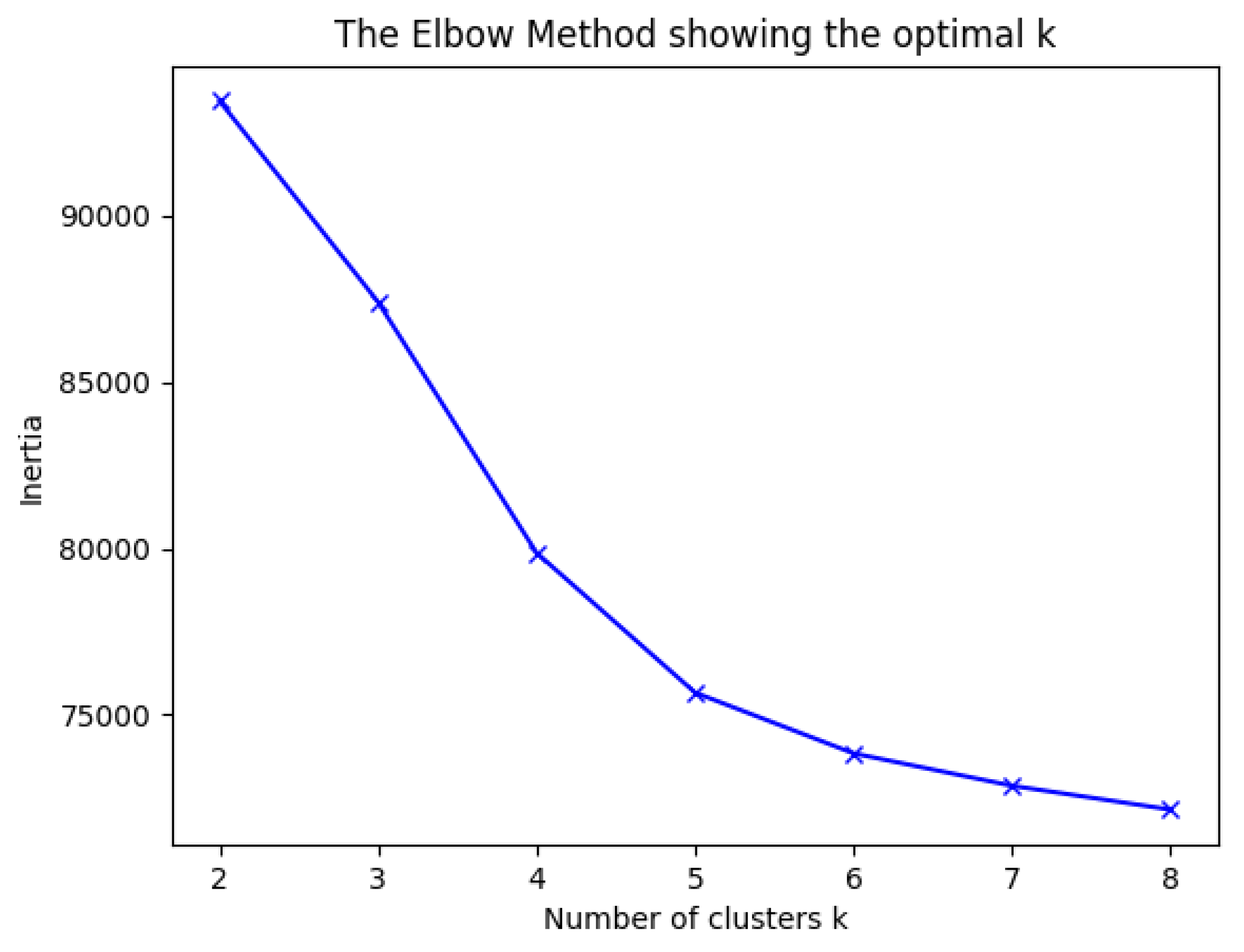
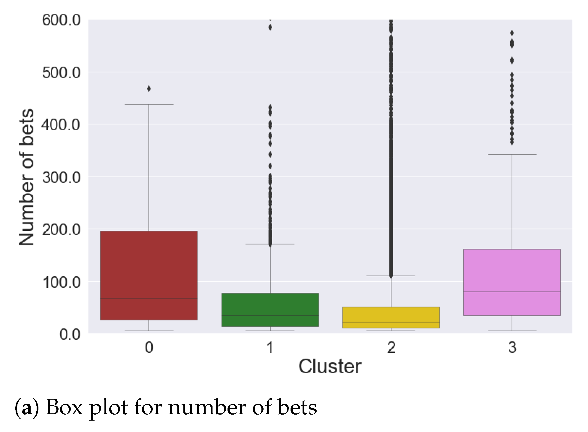
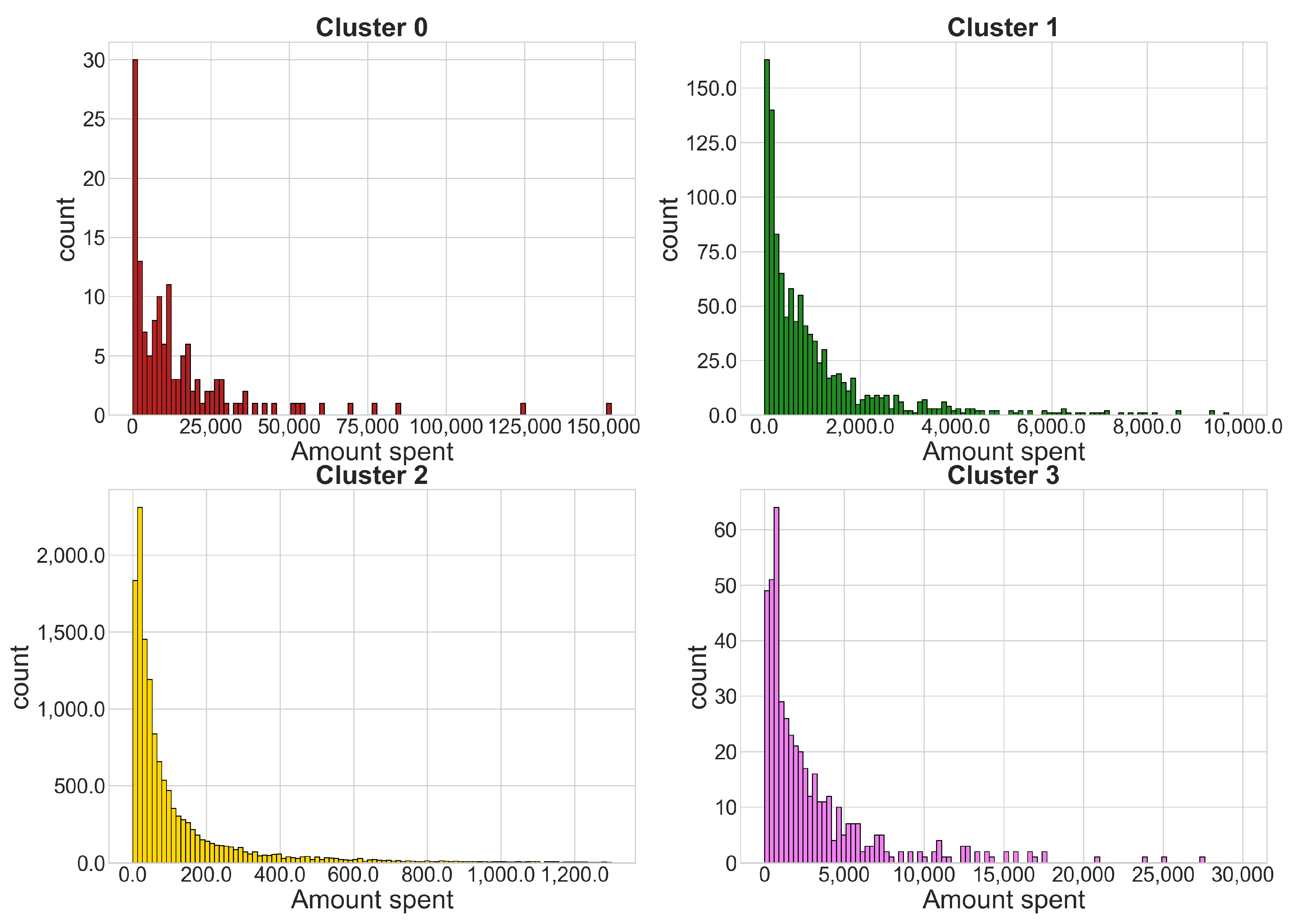
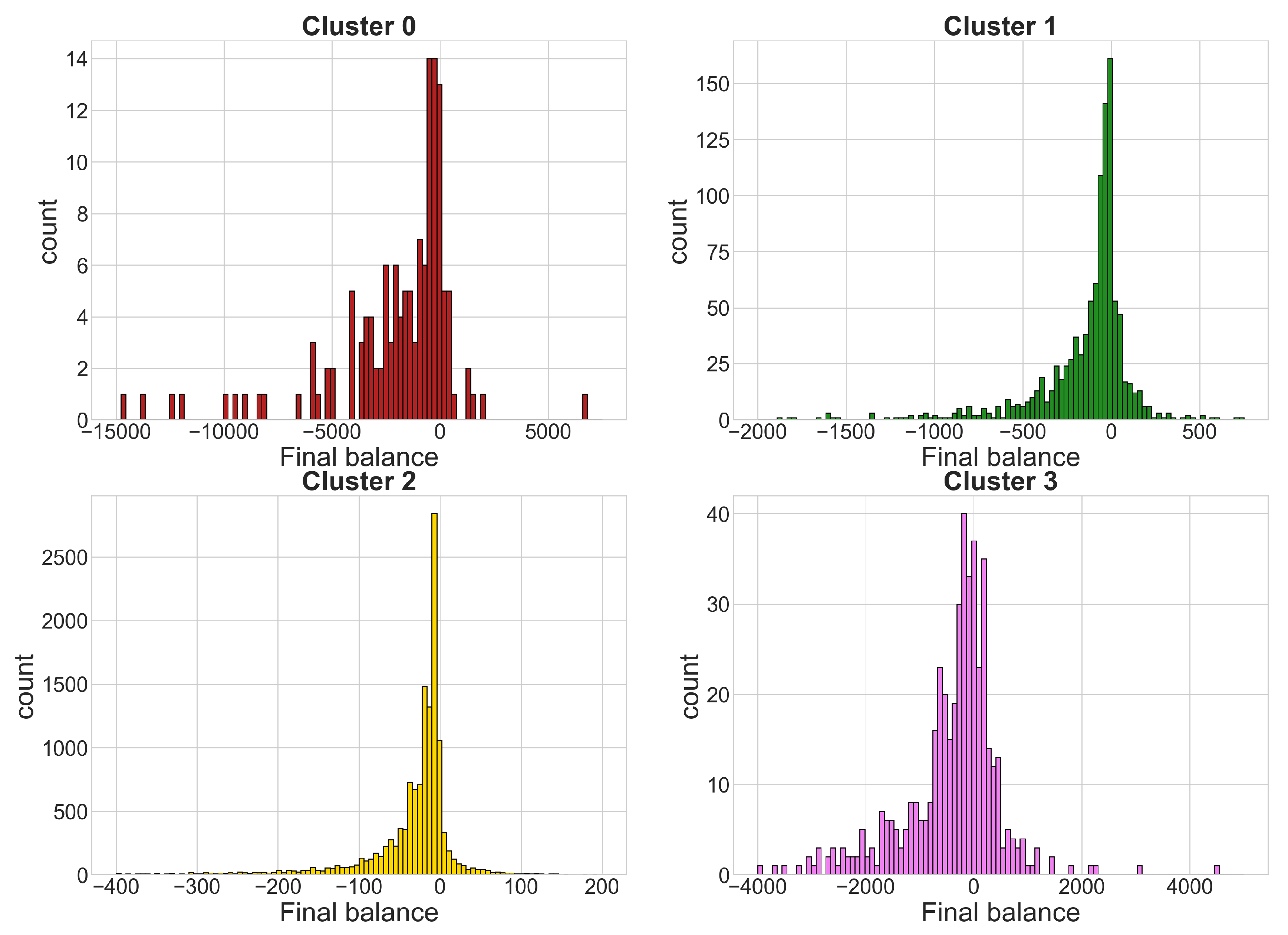
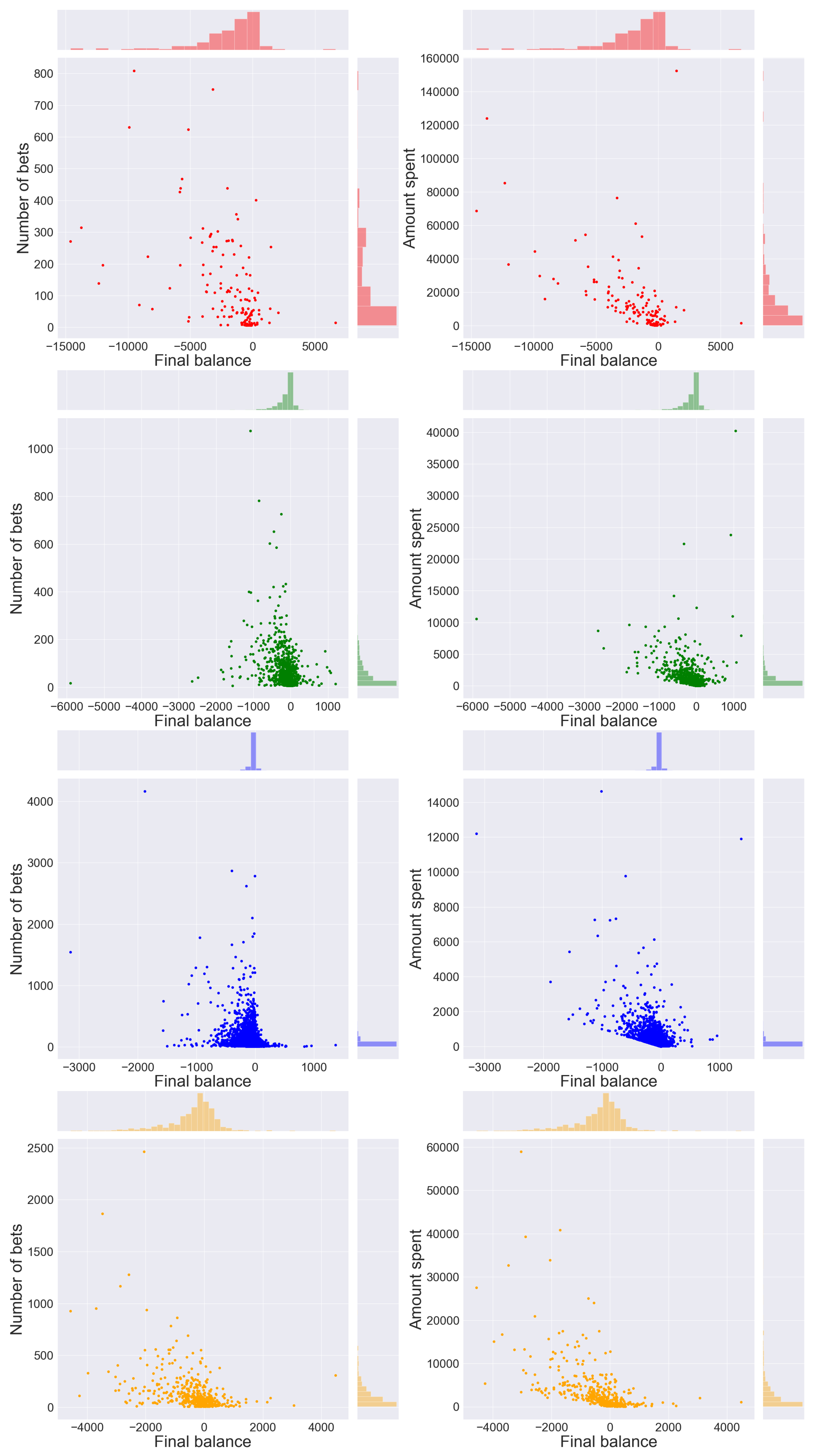
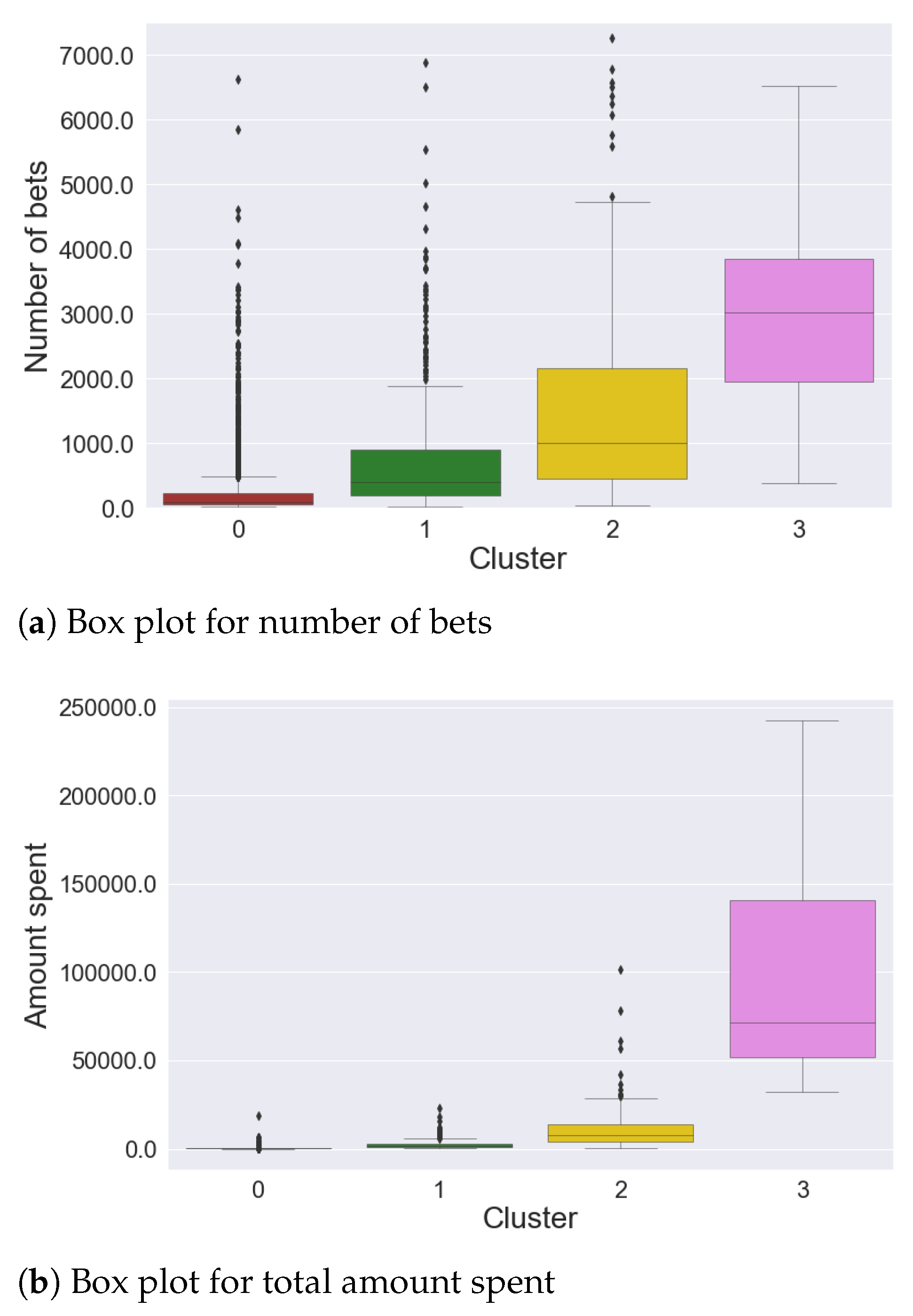
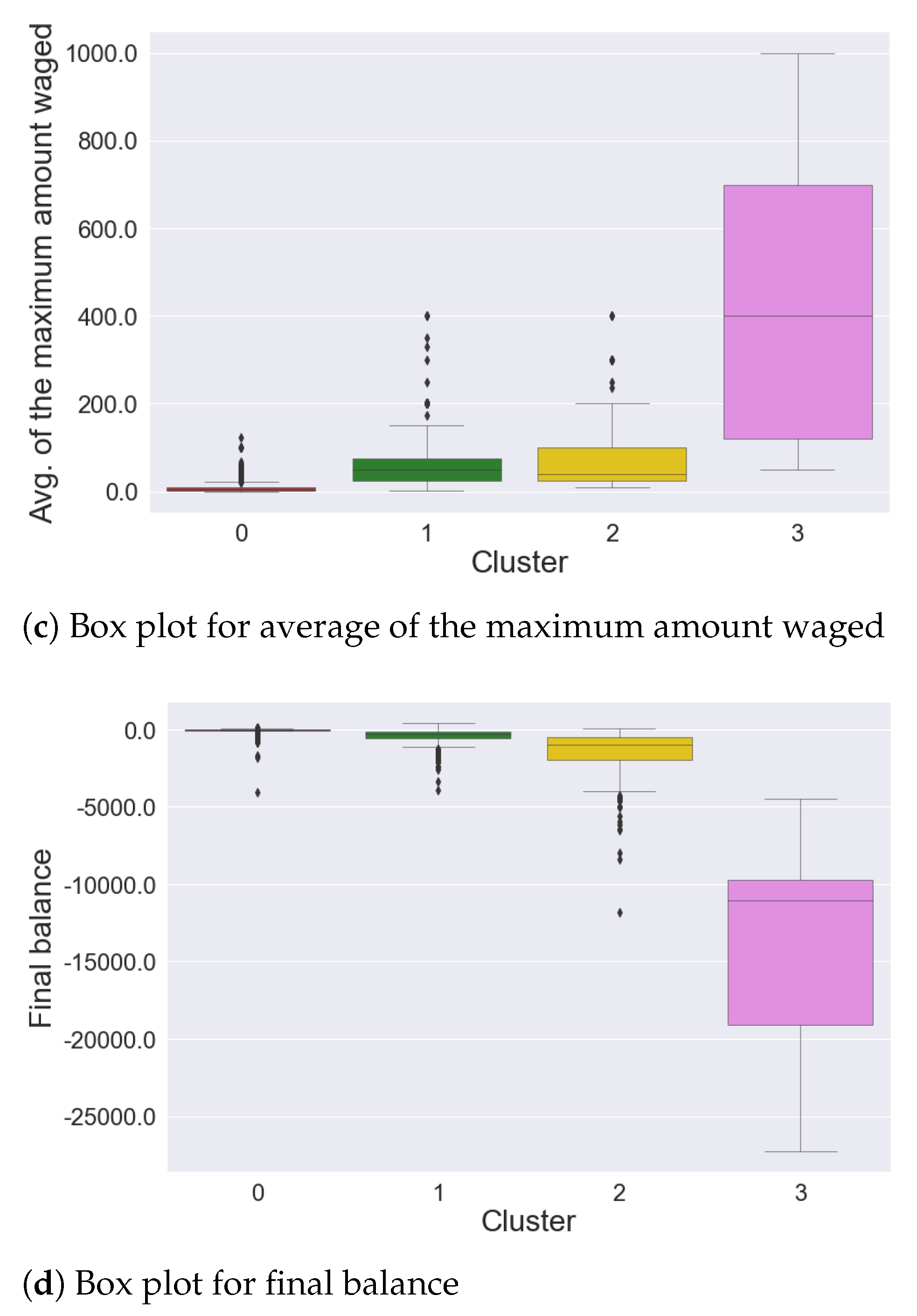
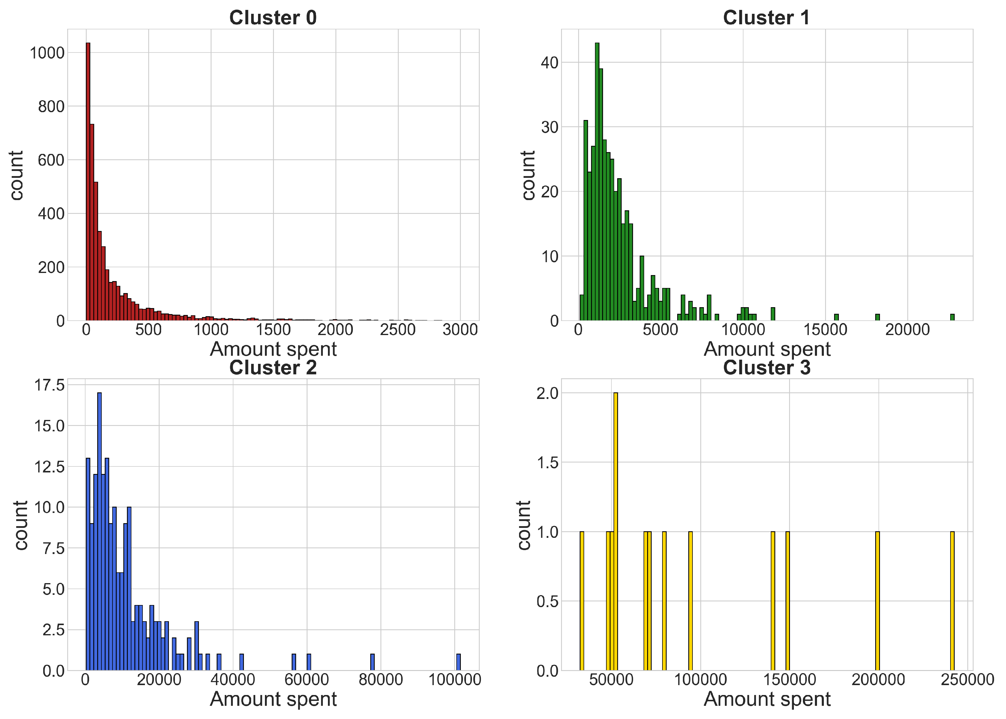
This section discusses the results obtained on the sports bets’ data set and on the black jack data set.

4.1. Sports Dataset

After obtaining the time series data set through the data preparation phase, the time series k-means algorithm was applied.
The elbow method was firstly executed to get an indication on the optimal number of clusters to form. As suggested in Figure 1, the most suitable values for k are four or five. Subsequently, the silhouette score was calculated for these two values, obtaining for k = 4 a value of 0.620 and for k = 5 a value of 0.317. These two positive values indicate that both clustering configurations are appropriate, but the first score is almost double with respect to the second one. For this reason, we selected k = 4 for executing the time series k-means algorithm.
After applying the algorithm, we obtained four clusters with observations distributed as follows:
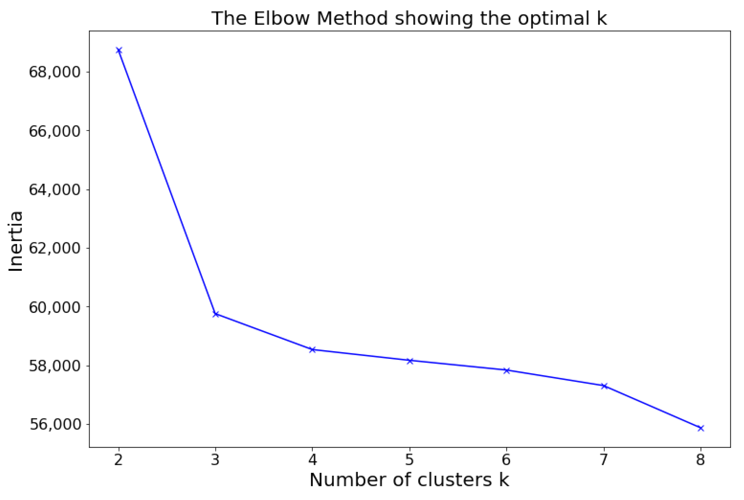
  • Cluster 0: 140 time series
  • Cluster 1: 1086 time series
  • Cluster 2: 13,390 time series
  • Cluster 3: 467 time series
Figure 2 shows, for each cluster, the box plots related to the number of bets placed, the total amount spent, the average of the maximum amount waged, and the final balance of a player. As one can see, the number of bets placed by a player is significantly higher in Clusters 0 and 3, with respect to Clusters 1 and 2. Similarly, the total amount spent on bets presents the same kind of behavior. This is a first indication that Clusters 0 and 3 are composed of players with a high propensity to play. However, there is a fundamental difference between these two groups: players belonging to Cluster 0 tend to bet much more money, as confirmed by the box plots related to the total amount spent and the maximum amount waged. Players who form Clusters 1 and 2, on the other hand, tend to place fewer bets with relatively low amounts. We could therefore say that Cluster 1 contains occasional players and Cluster 2 regular players who do not exaggerate the number of bets placed and amounts spent. Another important thing to notice comes from the box plot of final balances: occasional and regular players tend to gain or lose relatively small amounts with an almost symmetrical distribution with respect to zero. On the other hand, most of the players that compose Clusters 0 and 3 tend to lose more money than the previous two clusters. However, the proportion of players with a negative balance is significantly higher in Cluster 0.
The indications obtained from the box plots are confirmed by the histograms presented in Figure 3, Figure 4 and Figure 5, which represent, for each cluster, the distributions of the number of bets placed, the total amount spent, and the final balance of a player. It is very interesting to observe in Figure 5 the distribution of the final balance in Cluster 0 and Cluster 3, which clearly highlights a greater presence of looser gamblers in Cluster 0.
It is also important to inspect the relationships of the final balance with respect to the number of bets placed and the amount spent presented in Figure 6. From these plots, we can observe two things:
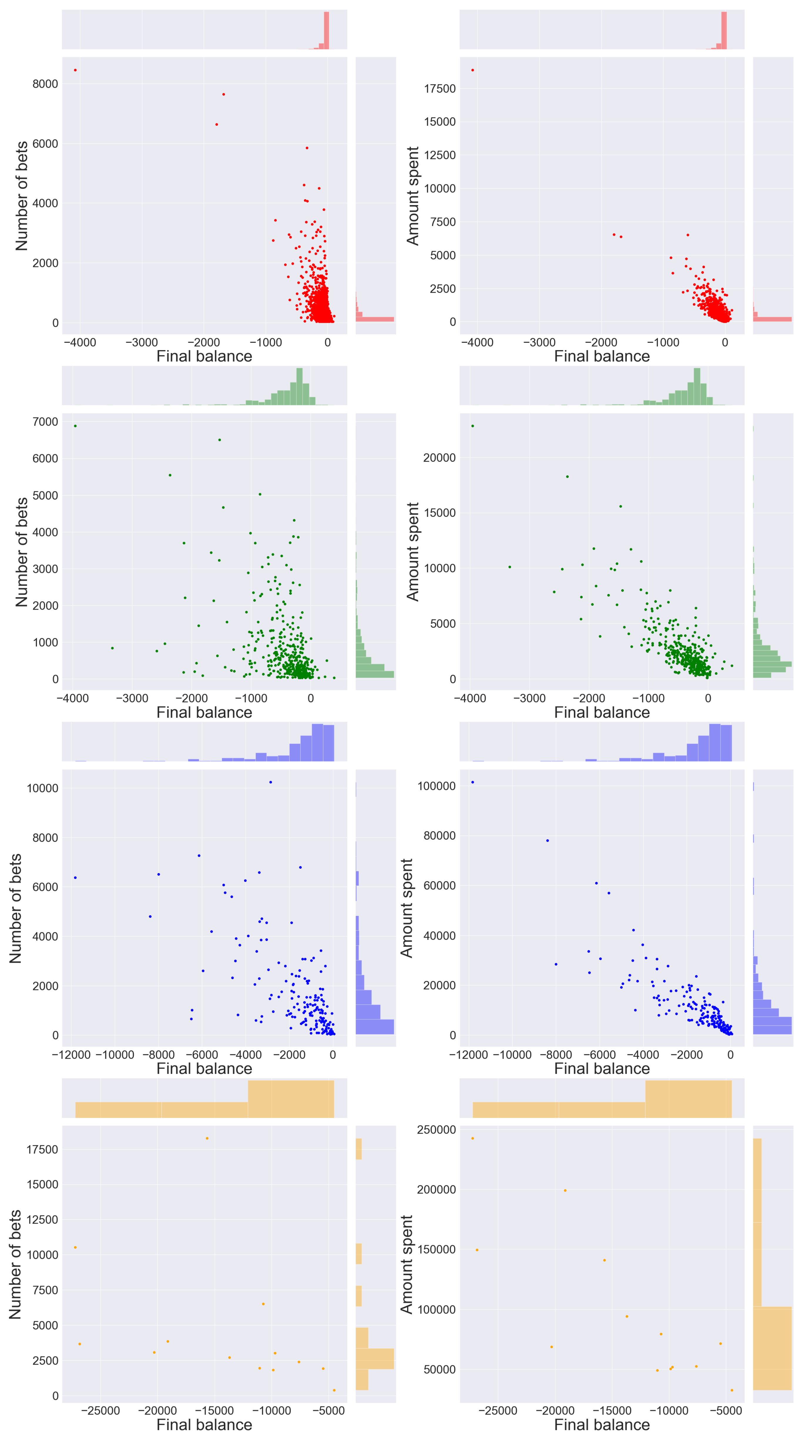
  • gamblers who have a positive balance tend to have a low number of placed bets, while only a few players who place many bets actually win.
  • gamblers who have a positive balance tend to have a lower amount spent compared to most players in the same cluster; only a few players who invest much money get a positive balance, which is usually very high.
From our point of view, it is not correct to label Cluster 0 as the one related to pathological gamblers and Cluster 3 as the one related to professional players, as both clusters show similar characteristics in terms of “style of play”. It would be more appropriate to say that both clusters include both professional and pathological gamblers, who belong to one of the two clusters based on the “level” of the disease. Taking into account the highlighted characteristics of players in Cluster 0 (high number of bets and losses), it seems to be composed of a large fraction of potential high-risk pathological gamblers, who can be easily identified. On the other hand, we can say that Cluster 3 contains a large number of potential medium-risk pathological gamblers (high number of bets, but lower losses). This distinction is made because compulsive gambling can lead an individual to place an increasing number of bets with ever higher amounts.
Figure 7, Figure 8, Figure 9 and Figure 10 show two examples of time series for each cluster. From these graphs, the differences between gamblers in different clusters are very clear.
Figure 11 depicts four potential high-risk pathological gamblers of Cluster 0. These plots are very good examples of typical pathological player behaviors, as they show that the players place a large number of bets (even with large amounts) while they continue to lose.
Figure 12 shows the same type of behavior of two gamblers in Cluster 3 with the difference that the total amount spent is lower. To conclude, we can state that the time series k-means algorithm is particularly suitable for identifying high-risk pathological gamblers, as well as potential medium-risk pathological gamblers.
While we cannot be sure that every player in these two clusters is a pathological one (given the similarity to professional players), considering a longer period (i.e., one year), there would be a clearer distinction between professional and pathological players. In fact, over a long period, the professional player is expected to achieve a positive balance. Nonetheless, it is possible to perform a posterior evaluation of the suitability of the proposed clustering algorithm. Some of the users analyzed in this study, in a subsequent period, asked the SRIJ to be included in a list of self-excluded users (i.e., users that do not want to have access to gambling platforms because they recognize themselves as problematic gamblers). Interestingly, all these users were included in the cluster of potentially addicted gamblers by the algorithm. Thus, the system represents a valid option to control and protect those users who suffer from a gambling addiction. In particular, the gambling authority can suggest to the addicted gambler specific actions ranging from contacting helplines to medical advice from a specialist in gambling dependency pathologies.

4.2. Black Jack

The result discussed in this section were obtained with the procedure presented before. Thus, the elbow method and the silhouette score were used to select the optimal value for k, and subsequently, the k-means algorithm was executed.
The elbow method suggests that the possible optimal values for k are three or four, as shown in Figure 13. The silhouette score was then calculated for these two values, obtaining a value of 0.66 for k = 3 and a value of 0.693 for k = 4 . These two values are both positive and relatively high, indicating that the clustering configuration is good in both cases. However, the value for k = 4 turns out to be slightly higher, making it preferable to the value of k = 3 .
After applying the algorithm, we obtained four clusters with the following number of observations:
  • Cluster 0: 4575
  • Cluster 1: 415
  • Cluster 2: 174
  • Cluster 3: 13
Figure 14 shows the analogous box plots presented in the previous section, for the results related to black jack.
The first thing we can notice is that the number of placed bets in each cluster is much greater than in sports bets’ data. This is certainly due to the type of game being considered. Another consequence that derives from the considered type of game is the amount spent: black jack is a game that requires a greater economic availability even just to make a limited number of bets (as confirmed by Figure 15 and Figure 16). We can also note that the number of placed bets in Clusters 2 and 3 is significantly higher than in the other two. Cluster 3 seems to contain gamblers who place many high value bets, losing much money at the end of the month. Cluster 2 seems also to contain gamblers who place many bets; however, the bet amounts are lower than in Cluster 3. Despite this, it is also characterized by a large fraction of gamblers with a negative final balance. Similarly to sports bets’ data, we can say that Cluster 0 and Cluster 1 represent respectively occasional and regular players, given the number of placed bets, the amount spent, and the final balance.
These indications are confirmed by the histograms presented in Figure 15, Figure 16 and Figure 17. Figure 17 highlights an interesting fact: only a small percentage of players, in the considered period, achieved a positive final balance.
Almost all the winning gamblers are concentrated in Clusters 0 and 1. Only a few gamblers in Cluster 2 made a profit, while in Cluster 3, there are no winning gamblers. Furthermore, as happened with the results obtained in sports bets, gamblers who have a positive balance tend to have a low number of placed bets and a low amount spent, as highlighted in Figure 18.
Given the presented characteristics of Clusters 2 and 3, we can say that Cluster 2 is composed by potential medium-risk pathological gamblers, while Cluster 3 by potential high-risk pathological gamblers. It should be noted that both clusters could contain both pathological and professional gamblers. However, the total absence of players with a positive final balance makes their identification difficult.
Figure 19, Figure 20, Figure 21 and Figure 22 show two examples of time series for each cluster, highlighting the differences between gamblers in different clusters.
Figure 23 shows four potential high-risk pathological gamblers, while Figure 24 shows two potential medium-risk pathological gamblers. These six plots clearly show the pathological behavior of the considered players, with the only difference that gamblers in Cluster 2 tend to place a smaller number (but still high compared to Clusters 0 and 1) of bets with smaller amounts, on average.
We can therefore say that, even in this case, the time series k-means algorithm can identify high-risk and medium-risk pathological gamblers. In particular, a posterior assessment allowed us to discover that all the self-excluded users were included in the cluster of potentially addicted gamblers by the algorithm. This analysis cannot detect the presence of users that were erroneously placed in the potentially addicted gamblers. Still, it suggests the system’s suitability for detecting users deserving special attention from the gambling authority.

5. Conclusions

In 2012, the European Commission released a statement highlighting the need for regulatory policies to aid in the detection of pathological gambling behaviors, citing “a responsibility to protect those citizens and families who suffer from a gambling addiction.”
To answer this call, in this paper, we propose an ML-based system to identify different profiles of users, aiming at discovering the high-risk pathological gamblers. To tackle this problem, we rely on a K-means algorithm based on the dynamic time warping algorithm, a well-known technique that makes it possible to align and compare time series. Data provided by the Portuguese authority for the control of gambling activities were considered. In particular, the data represent one month of online gambling activities collected by ten gambling providers operating in Portugal. The data contain different kinds of gambling modalities, including sports and black jack bets’ data used in this paper.
After a preprocessing phase aimed at building the time series for each player and the subsequent choice of the algorithm’s parameter (i.e., the number of clusters to be formed), the clustering algorithm under the DTW was executed. The clusters created by the algorithm allowed for an analysis of the different users’ profiles. In particular, for both the considered gambling modalities (i.e., black jack and sports bets), four clusters were obtained. From the analysis of these clusters, it was possible to characterize the respective users’ profiles. In particular, we were able to “label” the four clusters as follows: professional players, occasional players, regular players, pathological gamblers. Interestingly, the number of players in the “pathological gamblers” matched the existing knowledge of the gambling authority concerning the spread of this phenomenon. Moreover, a subsequent analysis allowed identifying in this cluster some users that asked for a self-exclusion from betting activities (thus recognizing themselves as potentially pathological gamblers).
The results obtained suggest the suitability of the considered algorithm in identifying potentially critical players. In particular, the identification of critical clusters with a limited number of players may simplify the subsequent analysis of the gambling control authority, which can focus its efforts and resources on the analysis of a small fraction of users.
As future work, we plan to build a predictive model for each of the identified cluster. This would allow predicting the behavior of the users and detecting anomalous behaviors. This information may indicate that a specific user is at risk of developing pathological gambling, and it can be used by the gambling control authority for taking specific actions.

Author Contributions

F.P. designed and implemented the system; F.P. performed the data preprocessing; M.R., and P.E. provided the data; M.C. supervised the work; M.C. and A.P. provided funding; L.M. and E.F. executed the experiments; F.P. and E.F. analyzed the results; F.P., E.F., L.M., A.P., and M.C. wrote the paper. All authors have read and agreed to the published version of the manuscript.

Funding

This work was supported by national funds through FCT (Fundação para a Ciência e a Tecnologia) under project DSAIPA/DS/0022/2018 (GADgET). Aleš Popovič acknowledges the financial support from the Slovenian Research Agency (research core funding No. P5-0410). We acknowledge the CINECA award under the ISCRA initiative, for the availability of high performance computing resources and support.

Institutional Review Board Statement

Not applicable.

Informed Consent Statement

Not applicable.

Data Availability Statement

Data were provided by the Gambling Inspection and Regulation Service of Portugal. Due to the existing regulation, data cannot be made available.

Conflicts of Interest

The authors declare no conflict of interest.

Appendix A. Time Series Analysis

A time series is defined as a set of observations x t , each one being recorded at a specific time t. In this paper, one observation corresponds to the profit for a single bet in the time instant in which that bet is placed by a single user.
In general, an increasingly large part of the worlds’ data is in the form of time series. Time series analysis includes methods for analyzing temporal data to discover the inherent structure and condense information over temporal data, as well as the meaningful statistics and other characteristics of the data. In the context of data mining, pattern recognition, and machine learning, time series analysis can be used for clustering, classification, anomaly detection, or forecasting. In this paper, we aim at clustering together gamblers that share common behaviors. Thus, time series clustering is the best and well-suited set of methods for our problem, since it has the goal of partitioning time series data into groups based on similarity or distance measures, so that time series in the same cluster are similar.
One major problem that arises during time series clustering, and in general in time series analysis, is the comparison of time series or sequences. The most studied approaches rely on proximity measures and metrics. Thus, a crucial question is establishing what we mean by “dissimilar” data objects. This concept is particularly complex due to the dynamic character of the series, and different approaches to define the (dis)similarity between time series have been proposed in the literature [18].
In particular, Euclidean distance and its variants, like the Minkowski distance, present several drawbacks that make their use in our application inappropriate. They compare only time series of the same length, which turns out to be unlikely due to the nature of our problem, as the number of bets varies from player to player. Additionally, they do not handle outliers or noise, and they are very sensitive with respect to six signal transformations: shifting, uniform amplitude scaling, uniform time scaling, uniform bi-scaling, time warping, and non-uniform amplitude scaling [19].
For this reason, this paper relies on dynamic time warping to determine the best alignment among time series.

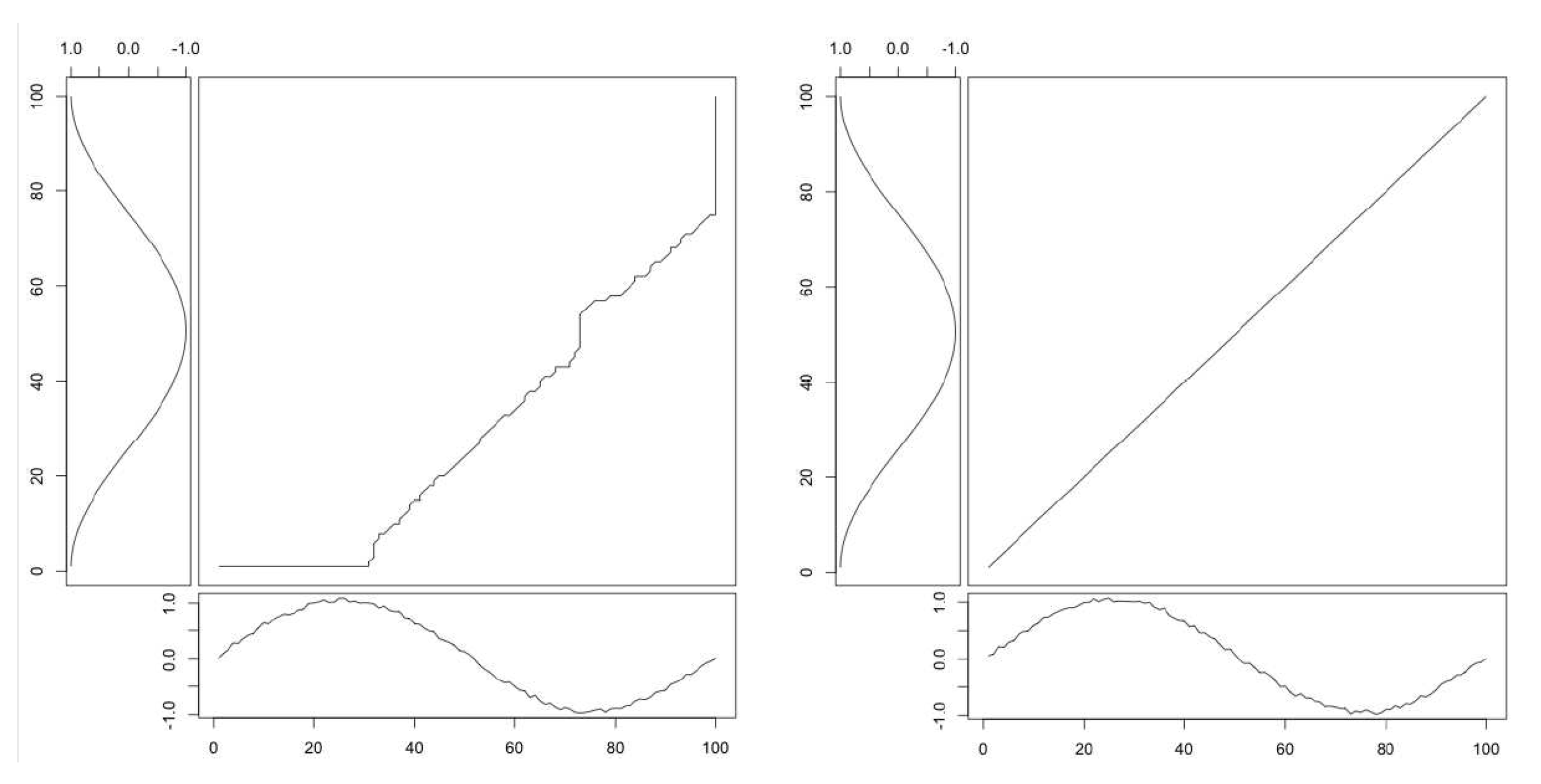
Appendix A.1. Dynamic Time Warping

One of the leading techniques in finding the best alignment is Dynamic Time Warping (DTW) [15,16,17].
DTW finds the optimal alignment between two time series and captures flexible similarities by aligning the elements inside both sequences. It finds the optimal alignment (or coupling) between two sequences of numerical values and captures flexible similarities by aligning the coordinates inside both sequences. It represents a generalization of the Euclidean distance, which allows a non-linear mapping of one time series to another one by minimizing the distance between both. DTW does not require that the two time series data have the same length, and it can handle local time-shifting by duplicating (or re-sampling) the previous element of the time sequence.
Let X = { x i } i = 1 N be a set of time series x i = ( x i 1 , , x i t ) assumed of length T (this assumption is only for the ease of explanation, since DTW can be applied equally on time series of equal or different lengths). An alignment π of length m between X i and x j is defined as the set of m couples of aligned elements of x i to elements of x j , with T m 2 T 1 , which means:
π = ( ( π 1 ( 1 ) , π 2 ( 1 ) ) , , ( π 1 ( m ) , π 2 ( m ) ) )
The alignment π defines a warping function, which creates a mapping from the time axis of x i into the time axis of x j and the applications π 1 and π 2 , defined from { 1 , , m } to { 1 , , T } . The following conditions are satisfied:
Condition 1.
Monotonicity
1 = π 1 ( 1 ) π 1 ( 2 ) π 1 ( m ) = T ,   1 = π 2 ( 1 ) π 2 ( 2 ) π 2 ( m ) = T
Intuitively, monotonicity defines that π 1 and π 2 can never “go back” in time.
Condition 2.
Boundary
π 1 ( l + 1 ) π 1 ( l ) + 1   a n d   π 2 ( l + 1 ) π 2 ( l ) + 1
( π 1 ( l + 1 ) π 1 ( l ) ) + ( π 2 ( l + 1 ) π 2 ( l ) ) 1 l { 1 , , m }
The first part of the boundary condition intuitively states that moving forward by one in time corresponds to a step of at most one in the π 1 and π 2 functions. The second condition states that moving forward by one in time forces at least one between π 1 and π 2 to also “move forward”.
Thus, an alignment π defines a way to associate all elements of x i and x j in which discrete steps in time correspond to either moving forward in x i , x j , or both.
The DTW between two time series x i and x j is defined as:
DTW ( x i , x j ) = min π A 1 π ( t , t ) π ϕ ( x i t , x j t )
where ϕ : R × R R + is a positive, real-valued, divergence function, usually the Euclidean norm, and A is the set of all possible alignments between x i and x j .
DTW is a dissimilarity measure on time series that makes it possible to capture temporal distortions, since its alignments deal with delays or time-shifting, whereas Euclidean alignments align elements observed at the same time. Boundary, monotonicity, and continuity are three important properties that are applied to the construction of the path. The boundary condition imposes that the first elements of the two time series are aligned to each other, as well as the last sequence’s elements. Monotonicity preserves the time-ordering of elements, meaning that the alignment path does not go back in the “time” index. Continuity limits the warping path from long jumps, and it guarantees that alignment does not omit important features.
It is also worth mentioning that DTW does not follow the triangle inequality; thus, it is a non-metric distance:
DTW ( x i , x j ) + DTW ( x j , x k ) DTW ( x i , x k )
As an example of the effect of DTW, Figure A1 shows the optimal alignment path with and without considering the time warping.
Figure A1. Optimal alignment path between two sample time series with time warping (left), without time warping (right).
Applsci 11 02397 g0a1

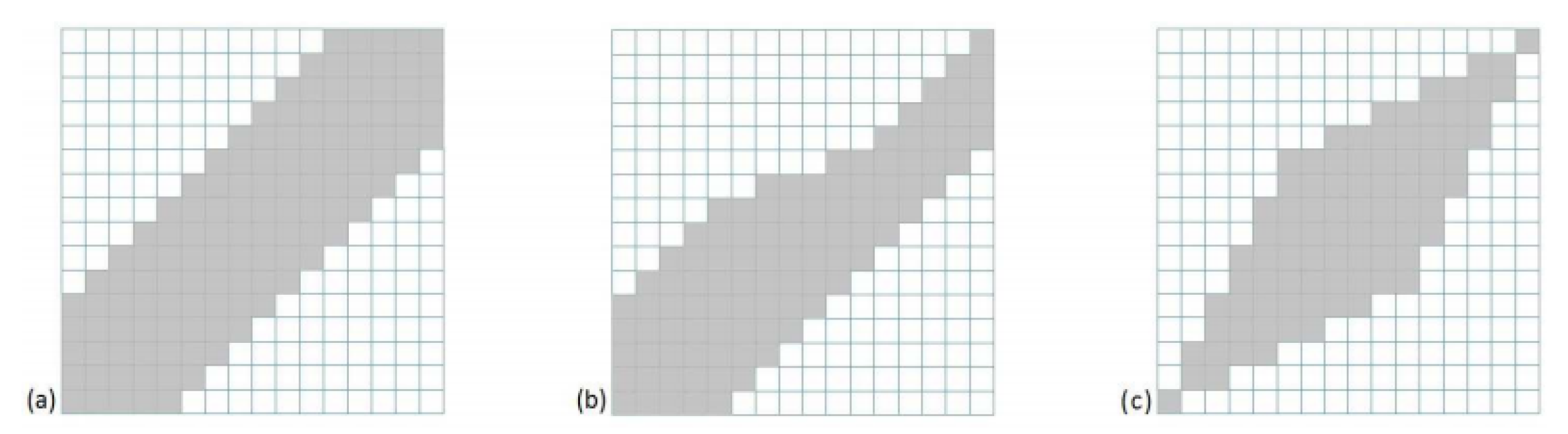
Appendix A.2. Constrained DTW

The time and space complexity of DTW is O ( N 2 ) , because each cell in the cost matrix is filled once in constant time, and the cost of the optimal alignment can be recursively computed by:
D ( t , t ) = d ( t , t ) + min D ( t 1 , t ) D ( t 1 , t 1 ) D ( t , t 1 )
The complexity of DTW is, usually, not an issue. Nevertheless, the “conventional” algorithm is too slow for searching an alignment path for a large data set. To improve the time and space complexity, as well as accuracy of DTW, different techniques for aligning time series have been introduced [20,21]. In this paper, we rely on the constrained DTW [22].
In constrained DTW, some constraints are used to speed up the original algorithm. The Sakoe–Chiba band [23] and Itakura parallelogram [16] are well-known constraints. The cost matrix is filled only in the shaded areas around the diagonal by DTW. These shaded areas depend on the constraint, as shown in Figure A2. Thus, the algorithm finds the optimal alignment according to the selected constrained window. It is fundamental to notice that the globally optimal alignment is found only if it is fully inside the window.
Figure A2. (a) Sakoe–Chiba band, (b) asymmetric Sakoe–Chiba band, and (c) Itakura parallelogram.
Applsci 11 02397 g0a2
Sakoe–Chiba DTW ( DTW s c ) is defined as follows:
DTW s c ( x i , x j ) min π A C ( π ) , C ( π ) 1 | π | k = 1 | π | w π 1 ( k ) , π 2 ( k ) ϕ ( x π 1 ( k ) i , x π 2 ( k ) j ) = 1 | π | ( t , t ) π w t , t ϕ ( x i t , x j t )
where if | t t | < c , then w t , t = 1 , and else , function ϕ is the Euclidean norm and c is the Sakoe–Chiba bandwidth.
Itakura DTW slightly differs from the Sakoe–Chiba version, since, instead of using the boundary condition introduced by Sakoe and Chiba, it imposes that two consecutive horizontal and vertical moves are not allowed. This is done by introducing an indicator function g ( · ) in the boundary constraints, for horizontal moves, and introducing a set of three actions for vertical ones. As a consequence, the algorithm is controlled to search through only a parallelogram space. In the DTW literature, the resulting search space is often called the “global” Itakura parallelogram, and the role of the indicator function g ( · ) is called the Itakura “local” constraint.

Appendix A.3. Time Series Averaging and Centroid Estimation

Averaging a set of time series, which is a fundamental and necessary task in clustering, needs to address the problem of multiple temporal alignments. A standard way to average two time series, under time warping, is to synchronize them and average each pairwise temporal warping alignment. The problem increases in complexity if there is the need to perform multiple alignment, since there is the need to determine a multiple alignment that links simultaneously all the time series on their commonly shared similar elements.
There are three different approaches to determine a multiple alignment: dynamic programming, progressive, and iterative.
Dynamic programming approaches search the optimal path within an N-dimensional grid that crosses the N time series. Progressive approaches progressively combine pairs of time series centroids to estimate the global centroid. Iterative approaches works similarly to the progressive approach, but they also reduce the error propagation problem, which arises when early errors propagate in all subsequent centroids through the pairwise combinations, by repeatedly refining the centroid and realigning it to the initial time series. This work focuses on iterative approaches that have a heuristic nature and are limited to the dynamic time warping metric. In particular, the paper uses the DTW Barycenter Averaging (DBA) [24] described in the following section.
Under DTW, given the time series x i , x j and their DTW alignment π * , the centroid c ( x i , x j ) is defined by averaging their aligned elements as:
c ( x i , x j ) = ( AVG ( x π 1 * ( 1 ) i , x π 2 * ( 1 ) j ) , , ( AVG ( x π 1 * ( m ) i , x π 2 * ( m ) j )
where AVG ( · ) is a standard numerical averaging function. The length T m 2 T 1 of a centroid c ( x i , x j ) is generally higher than the length of the centered time series.
Let X = { x 1 , , X N } be a set of time series x i = ( x i 1 , , x i T , i { 1 , , N } and S the space of all time series sequences. s S , the average sequence c should satisfy:
i N DTW ( x i , c ) i N DTW ( x i , s )
Since no information on the length of the average sequence c is available, the search cannot be limited to sequences of a given length, so all possible length values for averages have to be considered.

Appendix A.4. DTW Barycenter Averaging

DBA is a global averaging method that consists of iteratively refining an initially average sequence (potentially arbitrary), in order to minimize its distance to the set of time series, with the aim of minimizing inertia as the sum of squared DTW distances from the average sequence to the set of time series.
More deeply, for each iteration, DBA works in two steps:
  • Computing DTW between each individual sequence and the temporary average sequence to be refined, in order to find associations between coordinates of the average sequence and coordinates of the set of sequences.
  • Updating each coordinate of the average sequence as the barycenter of coordinates associated with it during the first step.
Let S now be the set of sequences to be averaged, c = ( c 1 , , c T ) the the average sequence at iteration i, and c = ( c 1 , , c T ) the update of c at iteration i + 1 , for which we want to find the coordinates. The t t h coordinate of the average sequence c is defined as:
c t = barycenter ( assoc ( c t ) )
where the function assoc ( · ) links each coordinate of the average sequence to one or more coordinates of the sequences of S , and it is computed during DTW computation between c and each sequence of S . The barycenter ( · ) function is defined as:
barycenter ( X 1 , , X α ) = X 1 + + X α α
Then, by computing again DTW between the average sequence and all sequences of S , the associations created by DTW may change. As it is impossible to anticipate how these associations will change, the algorithm makes c iteratively converge. Algorithm A1 details the complete DBA procedure.
Algorithm A1: DBA.
Applsci 11 02397 i001
In the algorithm initialization, there are two major factors to consider: the length of the starting average sequence and the values of its coordinates. The upper bound of the initial average is T N , but such a length cannot reasonably be used. However, the inherent redundancy of the data suggests that a much shorter sequence can be adequate. In practice, a length around T (the length of the sequences to average) performs well. As concerns the optimal values of the initial coordinates, they are theoretically impossible to determine. In methods that require an initialization, like K-means clustering, a large number of heuristics have been developed, like randomized choice or using an element of the set of sequences to average.
DBA guarantees convergence: at each iteration, inertia can only decrease, since the new average sequence is closer (under DTW) to the elements it averages. If the update does not modify the alignment of the sequences, barycenters composing the average sequence will get closer to the coordinates of S . In the other case, if the alignment is modified, it means that DTW calculates a better alignment with a smaller inertia, which decreases in that case also.
The overall time complexity of the averaging process of N sequences, each one containing T coordinates, is thus:
Θ ( DBA ) = Θ ( I ( N × T 2 + N × T ) ) = Θ ( I × N × T 2 )
where I represents the number of operations.
For a deeper and complete overview of this algorithm, see [24].

Appendix A.5. K-Means for Time Series under DTW

The goal of clustering is to partition data, in our case time series, into groups based on similarity or distance measures, so that data in the same cluster are similar, while different data points belong to different groups.
Formally, the clustering structure is represented as a set of clusters C = { C 1 , , C k } of the data X, s.t.:
i = 1 k C i = X C i C j = , i j
The clustering methods can be classified according to the type of input data to the algorithm, the clustering criteria defining the similarity (dissimilarity) or distance between data points, and the theory and fundamental concepts. Here, we focus on k-means clustering, which is a partitioning method that uses an iterative way to create the clusters by moving data points from one cluster to another, based on a distance measure, starting from an initial partitioning. This algorithm is one of the most popular clustering algorithms, as it provides a good trade-off between the quality of the solution obtained and its computational complexity.
K-means requires that the number of clusters k will be pre-set by the user. A common approach to determine k is the elbow method, which follows a heuristic approach. The method consists of plotting the explained variation as a function of the number of clusters and picking the elbow of the curve as the number of clusters to use. This method follows the intuition that increasing the number of clusters will naturally improve the fit and explain more variation since there are more parameters (more clusters) to use, but that at some point, this is over-fitting, and the elbow reflects this.
Generally, k-means is a clustering method that aims to find k centroids, one for each cluster, that minimize the sum of the distance of each data point from its respective cluster centroid. It solves, for x i X :
argmin { C 1 , , C k } j = 1 k x i C j d ( x i , c j )
where C 1 , , C k are k non-overlapping clusters, c j is the representative of cluster C j , and d ( · ) is a distance function. In Algorithm A2 is presented the “classic” k-means algorithm.
The algorithm starts with an initial set of cluster centers, or centroids, c 1 , c 2 , , c k , chosen at random or according to some heuristic criteria. The clustering algorithm uses an iterative refinement technique, in which, in each iteration, each data point is assigned to its nearest cluster centroid. Then, the cluster centroids are re-calculated. The refinement steps are repeated until the centroids no longer move. The complexity of each iteration, performed on N data points, is linear: Θ ( k × N ) . This is one of the reasons for its popularity, but other reasons are the simplicity of implementation and speed of convergence.
The classical version of the algorithm uses the Euclidean distance as the base metric, which we have already proven to be unsuitable for time series data. In our project, we use a modified version of the algorithm, called time series K-means, which uses DTW as the core metric and DBA to compute the cluster centers (centroids), which leads to better clusters and centroids.
Algorithm A2: k-means clustering.
Applsci 11 02397 i002
In the algorithm, in the first step, the clusters gather time series of similar shapes, which is due to the ability of DTW to deal with time shifts. Second, centroids are computed as the barycenters with respect to DTW, using DBA; hence, they allow retrieving a sensible average shape whatever the temporal shifts in the cluster. It is pretty easy to introduce these modifications into k-means, as shown by the pseudo-code presented in Algorithm A3.
Algorithm A3: Time series k-means.
Applsci 11 02397 i003
The complete and actual implementation of this algorithm can be found inside the tslearn Python package https://tslearn.readthedocs.io/en/stable/index.html (accessed on 12 October 2020), on which we relied for the computation in this project.

References

  1. Schneider, S. Towards a comprehensive European framework on online gaming. Gaming Law Rev. Econ. 2013, 17, 6–7. [Google Scholar] [CrossRef]
  2. European Gambling and Betting Association. Market Reality; EGBA: Brussels, Belgium, 2016. [Google Scholar]
  3. Jensen, C. Money over misery: Restrictive gambling legislation in an era of liberalization. J. Eur. Public Policy 2017, 24, 119–134. [Google Scholar] [CrossRef]
  4. Cowlishaw, S.; Kessler, D. Problem gambling in the UK: Implications for health, psychosocial adjustment and health care utilization. Eur. Addict. Res. 2016, 22, 90–98. [Google Scholar] [CrossRef] [PubMed]
  5. Browne, M.; Greer, N.; Armstrong, T.; Doran, C.; Kinchin, I.; Langham, E.; Rockloff, M. The Social Cost of Gambling to Victoria; Victorian Responsible Gambling Foundation: North Melbourne, Australia, 2017.
  6. Coussement, K.; De Bock, K.W. Customer churn prediction in the online gambling industry: The beneficial effect of ensemble learning. J. Bus. Res. 2013, 66, 1629–1636. [Google Scholar] [CrossRef]
  7. Percy, C.; França, M.; Dragičević, S.; d’Avila Garcez, A. Predicting online gambling self-exclusion: An analysis of the performance of supervised machine learning models. Int. Gambl. Stud. 2016, 16, 193–210. [Google Scholar] [CrossRef]
  8. Ladouceur, R.; Shaffer, P.; Blaszczynski, A.; Shaffer, H.J. Responsible gambling: A synthesis of the empirical evidence. Addict. Res. Theory 2017, 25, 225–235. [Google Scholar] [CrossRef]
  9. Haeusler, J. Follow the money: Using payment behavior as predictor for future self-exclusion. Int. Gambl. Stud. 2016, 16, 246–262. [Google Scholar] [CrossRef]
  10. Philander, K.S. Identifying high-risk online gamblers: A comparison of data mining procedures. Int. Gambl. Stud. 2014, 14, 53–63. [Google Scholar] [CrossRef]
  11. Wood, R.T.; Wohl, M.J. Assessing the effectiveness of a responsible gambling behavioral feedback tool for reducing the gambling expenditure of at-risk players. Int. Gambl. Stud. 2015, 15, 1–16. [Google Scholar] [CrossRef] [Green Version]
  12. Auer, M.; Griffiths, M.D. An empirical investigation of theoretical loss and gambling intensity. J. Gambl. Stud. 2014, 30, 879–887. [Google Scholar] [CrossRef] [PubMed] [Green Version]
  13. Gustafson, J. Using Machine Learning to Identify Potential Problem Gamblers. Master’s Thesis, Umeå University, Umeå, Sweden, 2019. [Google Scholar]
  14. Auer, M.; Griffiths, M.D. Predicting limit-setting behavior of gamblers using machine learning algorithms: A real-world study of Norwegian gamblers using account data. Int. J. Ment. Health Addict. 2019, 1–18. [Google Scholar] [CrossRef] [Green Version]
  15. Rabiner, L.; Juang, B.H.; Lee, C.H. An overview of automatic speech recognition. In Automatic Speech and Speaker Recognition; Springer: Boston, MA, USA, 1996; pp. 1–30. [Google Scholar]
  16. Itakura, F. Minimum prediction residual principle applied to speech recognition. IEEE Trans. Acoust. Speech Signal Process. 1975, 23, 67–72. [Google Scholar] [CrossRef]
  17. Kruskal, J.B.; Liberman, M. The Symmetric Time-Warping Problem: From Continuous to Discrete. In Time Warps, String Edits, and Macromolecules—The Theory and Practice of Sequence Comparison; Sankoff, D., Kruskal, J.B., Eds.; CSLI Publications: Stanford, CA, USA, 1999; Chapter 4. [Google Scholar]
  18. Liao, T.W. Clustering of time series data—A survey. Pattern Recognit. 2005, 38, 1857–1874. [Google Scholar] [CrossRef]
  19. Cassisi, C.; Montalto, P.; Aliotta, M.; Cannata, A.; Pulvirenti, A. Similarity measures and dimensionality reduction techniques for time series data mining. Adv. Data Min. Knowl. Discov. Appl. 2012, 71–96. [Google Scholar] [CrossRef] [Green Version]
  20. Keogh, E.J.; Pazzani, M.J. Scaling up dynamic time warping for datamining applications. In Proceedings of the Sixth ACM SIGKDD International Conference on Knowledge Discovery and Data Mining, Boston, MA, USA, 20–23 August 2000; pp. 285–289. [Google Scholar]
  21. Salvador, S.; Chan, P. Toward accurate dynamic time warping in linear time and space. Intell. Data Anal. 2007, 11, 561–580. [Google Scholar] [CrossRef] [Green Version]
  22. Andrade-Cetto, L. Constrained Dynamic Time Warping. U.S. Patent 7,904,410, 8 March 2011. [Google Scholar]
  23. Sakoe, H.; Chiba, S. Dynamic programming algorithm optimization for spoken word recognition. IEEE Trans. Acoust. Speech Signal Process. 1978, 26, 43–49. [Google Scholar] [CrossRef] [Green Version]
  24. Petitjean, F.; Ketterlin, A.; Gançarski, P. A global averaging method for dynamic time warping, with applications to clustering. Pattern Recognit. 2011, 44, 678–693. [Google Scholar] [CrossRef]
Figure 1. Elbow method plot on sports bets’ data using the time series k-means algorithm.
Applsci 11 02397 g001
Figure 2. Box plots for sports bets’ data obtained using the time series k-means algorithm.
Applsci 11 02397 g002aApplsci 11 02397 g002b
Figure 3. Histograms of the number of bets obtained using the time series k-means algorithm. The x axis reports the number of bets, while the y axis shows the number of players that have performed that number of bets during the month.
Applsci 11 02397 g003
Figure 4. Histograms of the total amount spent obtained using the time series k-means algorithm. The x axis reports the amount spent, while the y axis shows the number of players that spent that amount during the month.
Applsci 11 02397 g004
Figure 5. Histograms of the total balance obtained using the time series k-means algorithm. The x axis reports the balance, while the y axis shows the number of players that obtained that balance during the month.
Applsci 11 02397 g005
Figure 6. Bivariate scatter plots obtained using the time series k-means algorithm. Each row of this figure highlights for a single cluster the relationships between the final balance-number of bets and the final balance-amount spent.
Applsci 11 02397 g006
Figure 7. Time series plot of two players in Cluster 0.
Applsci 11 02397 g007
Figure 8. Time series plot of two players in Cluster 1.
Applsci 11 02397 g008
Figure 9. Time series plot of two players in Cluster 2.
Applsci 11 02397 g009
Figure 10. Time series plot of two players in Cluster 3.
Applsci 11 02397 g010
Figure 11. Time series plot of four potential high-risk pathological gamblers.
Applsci 11 02397 g011
Figure 12. Time series plot of two potential medium-risk pathological gamblers.
Applsci 11 02397 g012
Figure 13. Elbow method plot on black jack data using the time series k-means.
Applsci 11 02397 g013
Figure 14. Box plots for black jack bets’ data using the time series k-means algorithm.
Applsci 11 02397 g014aApplsci 11 02397 g014b
Figure 15. Histograms of the number of bets obtained using the time series k-means algorithm. The x axis reports the number of bets, while the y axis shows the number of players that have performed that amount of bets during the month.
Applsci 11 02397 g015
Figure 16. Histograms of the total amount spent obtained using the time series k-means algorithm. The x axis reports the amount spent, while the y axis shows the number of players that have spent that amount during the month.
Applsci 11 02397 g016
Figure 17. Histograms of the total balance obtained using the time series k-means algorithm. The x axis reports the balance, while the y axis shows the number of players that obtained that balance during the month.
Applsci 11 02397 g017
Figure 18. Bivariate scatter plots obtained using the time series k-means algorithm. Each row of this figure highlight for a single cluster the relationships between the final balance-number of bets and the final balance-amount spent.
Applsci 11 02397 g018
Figure 19. Time series plot of two players in Cluster 0.
Applsci 11 02397 g019
Figure 20. Time series plot of two players in Cluster 1.
Applsci 11 02397 g020
Figure 21. Time series plot of two players in Cluster 2.
Applsci 11 02397 g021
Figure 22. Time series plot of two players in Cluster 3.
Applsci 11 02397 g022
Figure 23. Time series plot of four potential high-risk pathological gamblers.
Applsci 11 02397 g023
Figure 24. Time series plot of two potential medium-risk pathological gamblers.
Applsci 11 02397 g024
Table 1. Raw data set and processed data set.
Data Preparation
Type of Game# of Raw DatasetsTotal Size Raw DatasetsSize Final Dataset# of Time Series
Sports75.40 GB101 MB15,081
Black Jack5481 MB72.6 MB5177
Publisher’s Note: MDPI stays neutral with regard to jurisdictional claims in published maps and institutional affiliations.

