Adaptive Optimal Robust Control for Uncertain Nonlinear Systems Using Neural Network Approximation in Policy Iteration

Abstract

In this study, based on the policy iteration (PI) in reinforcement learning (RL), an optimal adaptive control approach is established to solve robust control problems of nonlinear systems with internal and input uncertainties. First, the robust control is converted into solving an optimal control containing a nominal or auxiliary system with a predefined performance index. It is demonstrated that the optimal control law enables the considered system globally asymptotically stable for all admissible uncertainties. Second, based on the Bellman optimality principle, the online PI algorithms are proposed to calculate robust controllers for the matched and the mismatched uncertain systems. The approximate structure of the robust control law is obtained by approximating the optimal cost function with neural network in PI algorithms. Finally, in order to illustrate the availability of the proposed algorithm and theoretical results, some numerical examples are provided.

1. Introduction

It is ineluctable to contain uncertain parameters and disturbances in practical systems due to modeling errors, external disturbances, and so on [1]. Thus, it is of great practical significance to study robust control of the uncertain systems. In recent years, the control problem of uncertain systems has been extensively studied. The literature on robust control of uncertain systems mainly includes linear systems and nonlinear systems. For the uncertain linear systems, algebraic Riccati equations (ARE) or linear matrix inequalities (LMI) were mostly used to deal with them in the classical research methods [2,3,4,5,6]. In this literature, both matched and mismatched systems were involved. For nonlinear systems, the early research methods include feedback linearization, fuzzy modeling, nonlinear $H_{\infty }$ control, and so on [7,8,9,10,11]. However, in recent decades, neural networks (NN) and PI in RL were used to approximate the robust control law numerically [12,13,14].

The PI method in RL was initially utilized to calculate the optimal control law for some deterministic systems. Werbos first proposed an idea of approximating the solution in Bellman’s equation using approximate dynamic programming (ADP) [15]. There have been many results of using the PI method to calculate the optimal control law for some deterministic systems [16,17,18,19]. There are two major benefits of using the PI algorithm to deal with such optimal problems. On the one hand, it can effectively solve some problems of the “curse of dimensionality” in engineering control [20]. On the other hand, it can be utilized to calculate the optimal control law without knowing the system dynamics. In the practice of engineering control, it is difficult to obtain system dynamics accurately. Therefore, it is a good choice to use the PI algorithm to solve unknown model control problems.

Within the last ten years, the PI method was also developed to calculate the robust controller for some uncertain systems, which is based on the optimal control method of robust control [21]. For an input constraint nonlinear system with continuous time, a novel RL-based algorithm was prosposed to deal with the robust control problem in [22]. Based on network structure approximation, an online PI algorithm was developed to solve robust control of a class of nonlinear discrete-time uncertain systems in [23]. Using a data-driven RL algorithm, a robust control scheme was developed for a class of completely unknown dynamic systems with uncertainty in [24]. In addition, there are many other examples of literature on robust control based on RL, such as [25,26,27]. In all the literature listed above, the solution to the Hamilton Jacobi Bellman (HJB) equation was approximated by neural network. In fact, solving the HJB equation is a key problem in optimal control problem [28]. The HJB equation is difficult to solve because it is a nonlinear partial differential equation. For a nonlinear system, the HJB equation is solved with neural network approximation in many cases. Meanwhile, for the linear system, ARE is used to solve it instead of a neural network. However, for all we know, most of the current studies have not considered the input uncertainty in system. The input uncertainty does exist in the actual control system.

In this study, a class of continuous-time nonlinear systems with internal and input uncertainties is considered. The main objective is to establish robust control laws for the uncertain systems. By solving the optimal control problem constructed, the robust control problem is converted into calculating an optimal controller. The online PI algorithms are proposed to calculate robust control by approximating the optimal cost with neural network. The convergence of the proposed algorithms is proved. Numerical examples are given to illustrate the availability of the method.

Our main contributions are as follows. First, more general uncertain nonlinear systems are considered, in which the uncertainty entered both the system and the input. For the matched and the mismatched uncertain systems, it is proved that the robust control can be converted into calculating an optimal controller. Second, the online PI algorithms are developed to solve the robust control problem. The neural network is utilized to approximate the optimal cost in PI algorithm, which fulfilled a difficult task of solving the HJB equation.

The rest of this paper is arranged as follows. We formulate the robust control problems and propose some basic results for the issues under consideration in Section 2. Solving the robust control problem is converted to calculate an optimal control law of a nominal or auxiliary system in Section 3 and Section 4. Based on approximating optimal cost with neural network, the online PI algorithms are developed to solve the robust control problem in Section 5. To support the proposed theoretical framework, we provide some numerical examples in Section 6. In Section 7, the study is concluded, and the scope for future research is discussed.

2. Preliminaries and Problem Formulation

Consider an uncertain nonlinear system as follows:

$$\begin{array}{c}\hfill \dot{x}\left(t\right)=f\left(x\left(t\right)\right)+\Delta f\left(x\left(t\right)\right)+[g\left(x\left(t\right)\right)+\Delta g\left(x\left(t\right)\right)]u\left(t\right),x\left(0\right)=x_0\end{array}$$

(1)

where $x\left(t\right)\in {\mathbb{R}}^n$ is the system state, $u\left(t\right)\in {\mathbb{R}}^m$ is the control input, $f\left(x\left(t\right)\right)\in {\mathbb{R}}^n$, $g\left(x\left(t\right)\right)\in {\mathbb{R}}^{n\times m}$ are known function, $\Delta f\left(x\left(t\right)\right)\in {\mathbb{R}}^n$, $\Delta g\left(x\left(t\right)\right)\in {\mathbb{R}}^{n\times m}$ are uncertain disturbing function.

The control objective is to establish a robust control law $u=u\left(x\right)$ in order that the closed-loop system is asymptotically stable for all allowed uncertain disturbances $\Delta f\left(x\right(t\left)\right)$ and $\Delta g\left(x\right(t\left)\right)$.

As a general case, we first make the following assumptions to ensure that the state Equation (1) is well defined [1,29].

Assumption 1.

In (1), $f\left(x\right)+g\left(x\right)u$ is Lipschitz continuous with respect to x and u on the set $\Omega \subseteq {\mathbb{R}}^n$ containing the origin.

Assumption 2.

For the free vibration system, $f\left(0\right)=0,\Delta f\left(0\right)=0$, that is, $x=0$ is the equilibrium point of the free vibration system.

Definition 1.

The system (1) is called to satisfy the system dynamics matched condition if there is a function matrix $h\left(x\right)\in R^{m\times 1}$ such that

$$\Delta f\left(x\right)=g\left(x\right)h\left(x\right).$$

(2)

Definition 2.

System (1) is called to satisfy the input matched condition if there is a function $m\left(x\right)\in R^{m\times m}$ such that

$$\Delta g\left(x\right)=g\left(x\right)m\left(x\right),$$

(3)

where $m\left(x\right)\ge 0$.

Definition 3.

If the system (1) satisfies the conditions (2) and (3) for any allowed disturbances $\Delta f\left(x\right)$ and $\Delta g\left(x\right)$, then the system (1) is called a matched uncertain system.

Definition 4.

If the system (1) does not satisfy the condition (2) or (3) for any allowed disturbances $\Delta f\left(x\right)$ and $\Delta g\left(x\right)$, then the system (1) is called a mismatched uncertain system.

Next, we consider the robust control problem of nonlinear system (1) with matched and mismatched conditions, respectively.

3. Robust Control of Matched Uncertain Nonlinear Systems

This section considers the problem of robust control when the system (1) meets the matched conditions (2) and (3). By constructing appropriate performance indexes, the problem of robust control is transformed into calculating the optimal control law of a corresponding nominal system. Based on the optimal control of the nominal system, a PI algorithm is proposed to obtain robust feedback controller.

For the nominal system

$$\begin{array}{c}\hfill \dot{x}=f\left(x\right)+g\left(x\right)u,\end{array}$$

(4)

find the controller $u=u\left(x\right)$ to minimize performance index

$$\begin{array}{c}\hfill J(x_0,u)={\int }_0^{\infty }[f_{max}^2\left(x\right)+x^{T}x+u^{T}u]dt\end{array}$$

(5)

where $f_{max}\left(x\right)$ is the supremum function of uncertainty $h\left(x\right)$, that is $\parallel h\left(x\right)\parallel \le f_{max}\left(x\right)$.

The definition of admissible control in optimal control problem is given below [26].

Definition 5.

The control policy $u\left(x\right)$ is called an admissible control of the system (4) with regard to the performance function (5) on compact set $\Omega \subseteq {\mathbb{R}}^n$ if $u\left(x\right)$ is continuous on Ω, $u\left(0\right)=0$, it can stabilize the system (4) on $\Omega$, and the performance function (5) is limited for any $x\in \Omega$.

According to the performance index (5), the cost function corresponding to the admissible control $u\left(x\right)$ is given by

$$\begin{array}{c}\hfill V(x,u)={\int }_t^{\infty }[f_{max}^2\left(x\right)+x^{T}x+u^{T}u]dt\end{array}$$

(6)

Taking time derivative on both side of (6), it follows the Bellman equation

$$\begin{array}{c}\hfill f_{max}^2\left(x\right)+x^{T}x+u^{T}u+\nabla V^T[f\left(x\right)+g\left(x\right)u]=0,\end{array}$$

(7)

where $\nabla V$ is the gradient vector of the cost function $V(x,u)$ with respect to x.

Definite Hamiltonian function

$$\begin{array}{c}\hfill \begin{array}{c}\hfill H(x,u,\nabla V)=f_{max}^2\left(x\right)+x^{T}x+u^{T}u+\nabla V^T[f\left(x\right)+g\left(x\right)u]\end{array}\end{array}$$

(8)

Determining the extremum of the Hamiltonian function yields the optimal control function

$$\begin{array}{c}\hfill u^{*}\left(x\right)=-\frac{1}{2}{g}^T\left(x\right)\nabla V\end{array}$$

(9)

By substituting (9) into (7), it follows that optimal cost $V^{*}\left(x\right)$ satisfies the following HJB equation

$$f_{max}^2\left(x\right)+x^{T}x+\nabla V^{*T}f\left(x\right)-\frac{1}{4}\nabla V^{*T}g\left(x\right)g^T\left(x\right)\nabla V^{*}=0$$

(10)

and initial conditions $V^{*}\left(0\right)=0$.

Solving the optimal cost $V^{*}\left(x\right)$ from the HJB Equation (10), we can get the solution to the optimal control problem. Thus, the robust control problem can be solved.

The following theorem shows that optimal control $u^{*}\left(x\right)=-\frac{1}{2}{g}^T\left(x\right)\nabla V^{*}$ is a robust controller for matched uncertain systems.

Theorem 1.

Assume that the conditions (2) and (3) hold in system (1) and the solution $V^{*}\left(x\right)$ in HJB Equation (10) exists. Considering the nominal nonlinear system (4) with performance index (5), then the optimal control policy $u^{*}\left(x\right)=-\frac{1}{2}{g}^T\left(x\right)\nabla V^{*}$ can globally asymptotically stabilize the nonlinear uncertain system (1). That is to say, the closed-loop uncertain system $\dot{x}\left(t\right)=f\left(x\left(t\right)\right)+\Delta f\left(x\left(t\right)\right)+[g\left(x\left(t\right)\right)+\Delta g\left(x\left(t\right)\right)]u^{*}\left(x\right)$ is globally asymptotically stable.

Proof. 

In order to prove the stability with controller $u^{*}\left(x\right)=-\frac{1}{2}{g}^T\left(x\right)\nabla V^{*}$, $V^{*}\left(x\right)$ is chosen as the Lyapunov function. Considering the performance index (5), $V^{*}\left(x\right)$ is obviously positive, and $V^{*}\left(0\right)=0$. Taking time derivative of the function $V^{*}\left(x\right)$ along closed-loop system (1), it follows that

$$\begin{array}{c}\hfill \begin{array}{c}\hfill \frac{d{V}^{*}}{dt}=\nabla V^{*T}[f\left(x\right)+\Delta f\left(x\right)]-\frac{1}{2}\nabla V^{*T}[g\left(x\right)+\Delta g\left(x\right)]g^T\left(x\right)\nabla V^{*}\end{array}\end{array}$$

(11)

Using the matched conditions (2)and (3), it follows from (11) that

$$\begin{array}{c}\hfill \begin{array}{cc}\hfill \frac{d{V}^{*}}{dt}=& \nabla V^{*T}f\left(x\right)+\nabla V^{*T}g\left(x\right)h\left(x\right)-\frac{1}{2}\nabla V^{*T}g\left(x\right)g^T\left(x\right)\nabla V^{*}\hfill \\ & -\frac{1}{2}\nabla V^{*T}g\left(x\right)m\left(x\right)g^T\left(x\right)\nabla V^{*}\hfill \end{array}\end{array}$$

(12)

From HJB Equation (10), one can obtain

$$\begin{array}{c}\hfill \nabla V^{*T}f\left(x\right)=-f_{max}^2\left(x\right)-x^{T}x+\frac{1}{4}\nabla V^{*T}g\left(x\right)g^T\left(x\right)\nabla V^{*}\end{array}$$

(13)

Substituting (13) into (12) yields

$$\begin{array}{c}\hfill \begin{array}{cc}\hfill \frac{d{V}^{*}}{dt}=& -f_{max}^2\left(x\right)-x^{T}x+\frac{1}{4}\nabla V^{*T}g\left(x\right)g^T\left(x\right)\nabla V^{*}+\nabla V^{*T}g\left(x\right)h\left(x\right)-\frac{1}{2}\nabla V^{*T}g\left(x\right)g^T\left(x\right)\nabla V^{*}\hfill \\ & -\frac{1}{2}\nabla V^{*T}g\left(x\right)m\left(x\right)g^T\left(x\right)\nabla V^{*}\hfill \\ \hfill =& -f_{max}^2\left(x\right)-x^{T}x-\frac{1}{4}\nabla V^{*T}g\left(x\right)g^T\left(x\right)\nabla V^{*}+\nabla V^{*T}g\left(x\right)h\left(x\right)-\frac{1}{2}\nabla V^{*T}g\left(x\right)m\left(x\right)g^T\left(x\right)\nabla V^{*}\hfill \end{array}\end{array}$$

(14)

It follows from $m\left(x\right)\ge 0$ that $-\frac{1}{2}\nabla V^{*T}g\left(x\right)m\left(x\right)g^T\left(x\right)\nabla V^{*}\le 0$. Therefore, from (14), we can have -4.6cm0cm

$$\begin{array}{c}\hfill \begin{array}{cc}\hfill \frac{d{V}^{*}}{dt}\le & -f_{max}^2\left(x\right)-x^{T}x-\frac{1}{4}\nabla V^{*T}g\left(x\right)g^T\left(x\right)\nabla V^{*}+\nabla V^{*T}g\left(x\right)h\left(x\right)\hfill \\ \hfill =& -f_{max}^2\left(x\right)-x^{T}x-\frac{1}{4}[\nabla V^{*T}g\left(x\right)g^T\left(x\right)\nabla V^{*}-4\nabla V^{*T}g\left(x\right)h\left(x\right)+4h{\left(x\right)}^{T}h\left(x\right)]+h{\left(x\right)}^{T}h\left(x\right)\hfill \\ \hfill =& -x^{T}x+h{\left(x\right)}^{T}h\left(x\right)-f_{max}^2\left(x\right)-\frac{1}{4}{[g^T\left(x\right)\nabla V^{*}-2h\left(x\right)]}^T[g^T\left(x\right)\nabla V^{*}-2h\left(x\right)]\hfill \\ \hfill \le & -x^{T}x\hfill \end{array}\end{array}$$

(15)

Therefore, by Lyapunov stability theory [30], the optimal control $u^{*}\left(x\right)=-\frac{1}{2}{g}^T\left(x\right)\nabla V^{*}$ can make the matched uncertain system (1) asymptotically stable. Thus, for a constant $c>0$, there is a neighborhood $N=\{x:\parallel x\parallel <c\}$ such that if the state $x\left(t\right)$ enters the neighborhood N, then $x\to 0$ when $t\to \infty$. However, $x\left(t\right)$ cannot stay out of the domain N forever; otherwise, for all $t>0$, there is $\parallel x\left(t\right)\parallel \ge c$. This implies that

$$\begin{array}{c}\hfill \begin{array}{cc}\hfill V^{*}\left[x\left(t\right)\right]-V^{*}\left[x\left(0\right)\right]& ={\int }_0^t{\dot{V}}^{*}\left(x\left(\tau \right)\right)dt\hfill \\ & \le {\int }_0^t(-x^{T}x)dt\hfill \\ & \le -{\int }_0^t{c}^{2}dt\hfill \\ & =-c^{2}t\hfill \end{array}\end{array}$$

Therefore, when $t\to \infty$, $V^{*}\left[x\left(t\right)\right]\le V^{*}\left[x\left(0\right)\right]-c^{2}t\to -\infty$. This contradicts that $V^{*}\left[x\left(t\right)\right]$ is positive definite. Consequently, the system (1) is globally asymptotically stable. □

Remark 1.

For matched nonlinear systems, the robust controller can be obtained by solving the optimal cost function $V^{*}\left[x\left(t\right)\right]$ from HJB Equation (10). In Section 4, we will use the PI algorithm to solve the HJB equation, which is a difficult partial differential equation.

4. Robust Control of Nonlinear Systems with Mismatched Uncertainties

In this section, we consider the robust control problem when the system (1) does not satisfy the matched condition (2). At this time, the system is a mismatched nonlinear uncertain system. By constructing the appropriate auxiliary system and performance index, the robust control for the mismatched uncertain system is transformed into solving optimal control law of an auxiliary system.

Firstly, the following assumptions are given.

Assumption 3.

Suppose that the uncertainty of system (1) satisfies $\Delta f\left(x\right)=c\left(x\right)h\left(x\right)$, $\Delta g\left(x\right)=g\left(x\right)m\left(x\right)$, where $c\left(x\right)$ is a known function matrix of appropriate dimensions, $h\left(x\right)$ and $m\left(x\right)$ are uncertain functions, and $m\left(x\right)\ge 0$.

The goal of robust control is to find a control function $u\left(x\right)$, which makes the closed-loop system

$$\begin{array}{c}\hfill \dot{x}=f\left(x\right)+c\left(x\right)h\left(x\right)+[g\left(x\right)+g\left(x\right)m\left(x\right)]u\left(x\right)\end{array}$$

(16)

globally asymptotically stable for all uncertainties $h\left(x\right)$ and $m\left(x\right)$.

In order to obtain the robust controller, an optimal control problem is constructed as follow. For the following auxiliary systems

$$\begin{array}{c}\hfill \dot{x}=f\left(x\right)+g\left(x\right)u+[I-g\left(x\right)g{\left(x\right)}^{+}]c\left(x\right)v\end{array}$$

(17)

find the controller $u=u\left(x\right)$, $v=v\left(x\right)$, such that the performance index

$$\begin{array}{c}\hfill \begin{array}{c}\hfill J(x_0,u)={\int }_0^{\infty }[f_{max}^2\left(x\right)+g_{max}^2\left(x\right)+{\beta }^2{x}^{T}x+u^{T}u+v^{T}v]dt\end{array}\end{array}$$

(18)

is minimized, where $\beta$ is the design parameter, $g{\left(x\right)}^{+}={\left[g^T\left(x\right)g\left(x\right)\right]}^{-1}{g}^T\left(x\right)$ is a pseudo inverse of the matrix function $g\left(x\right)$. Moreover, $f_{max}\left(x\right)$ and $g_{max}\left(x\right)$ are nonnegative functions and satisfy the conditions

$$\begin{array}{c}\hfill {\parallel g\left(x\right)}^{+}c\left(x\right)h\left(x\right)\parallel \le f_{max}\left(x\right),\parallel h\left(x\right)\parallel \le g_{max}\left(x\right)\end{array}$$

(19)

According to the performance index (18), the cost function corresponding to the admissible control $\left(u\right(x),v(x\left)\right)$ is

$$\begin{array}{c}\hfill \begin{array}{c}\hfill V\left(x\right)={\int }_t^{\infty }[f_{max}^2\left(x\right)+g_{max}^2\left(x\right)+{\beta }^2{x}^{T}x+u^{T}u+v^{T}v]dt\end{array}\end{array}$$

(20)

The following Bellman equation is obtained by taking the time derivation on both sides of (20)

$$\begin{array}{c}\hfill \begin{array}{c}\hfill f_{max}^2\left(x\right)+g_{max}^2\left(x\right)+{\beta }^2{x}^{T}x+{\overline{u}}^T\overline{u}+\nabla V^T[f\left(x\right)+\overline{g}\left(x\right)\overline{u}]=0,\end{array}\end{array}$$

(21)

where $\nabla V$ is the gradient vector of $V\left(x\right)$ with respect to x, $\overline{g}\left(x\right)=[g\left(x\right),(I-g\left(x\right)g{\left(x\right)}^{+})c\left(x\right)]$, $\overline{u}={[u^T,v^T]}^T$.

Defining Hamiltonian functions as

$$\begin{array}{c}\hfill \begin{array}{c}\hfill H(x,u,\nabla V)=f_{max}^2\left(x\right)+g_{max}^2\left(x\right)+{\beta }^2{x}^{T}x+{\overline{u}}^T\overline{u}+\nabla V^T[f\left(x\right)+\overline{g}\left(x\right)\overline{u}]\end{array}\end{array}$$

(22)

Assuming that the minimum value exists and is unique in (22), the optimal control law is given by

$$\begin{array}{c}\hfill \begin{array}{cc}\hfill {\overline{u}}^{*}\left(x\right)& =\left[\begin{array}{c}{u}^{*}\left(x\right)\\ v^{*}\left(x\right)\end{array}\right]=-\frac{1}{2}{\overline{g}}^T\left(x\right)\nabla V^{*}\hfill \\ & =-\frac{1}{2}\left[\begin{array}{c}{g}^T\left(x\right)\nabla V^{*}\\ c^T\left(x\right){[I-g\left(x\right)g{\left(x\right)}^{+}]}^T\nabla V^{*}\end{array}\right]\hfill \end{array}\end{array}$$

(23)

By substituting (23) into (21), the HJB equation is given by

$$\begin{array}{c}\hfill \begin{array}{c}\hfill f_{max}^2\left(x\right)+g_{max}^2\left(x\right)+{\beta }^2{x}^{T}x+\nabla V^{*T}f\left(x\right)-\frac{1}{4}\nabla V^{*T}\overline{g}\left(x\right){\overline{g}}^T\left(x\right)\nabla V^{*}=0\end{array}\end{array}$$

(24)

and the initial value $V^{*}\left(0\right)=0$.

Remark 2.

Generally, the pseudo-inverse of $g\left(x\right)$, $g{\left(x\right)}^{+}$ will exist if its columns are linearly independent when Assumptions 1 and 2 are true [31]. In practical control systems, the function, $g\left(x\right)$, is usually column full-rank. Therefore, the pseudo-inverse of the function $g\left(x\right)$ is generally satisfied. Furthermore, the pseudo-inverse $g{\left(x\right)}^{+}$ satisfies $g{\left(x\right)}^{+}g\left(x\right)=I$. However, it does not satisfy $g\left(x\right)g{\left(x\right)}^{+}=I$. In addition, the auxiliary system constructed above is not a nominal system, but a compensation control term $v\left(x\right)$ is added to the nominal system.

If we can choose an appropriate parameter $\beta$, the optimal cost $V^{*}\left(x\right)$ can be computed from HJB Equation (24). Then, we can get the optimal control law of system (17) with performance index (18). The following theorem shows that optimal control $u^{*}\left(x\right)=-\frac{1}{2}{g}^T\left(x\right)\nabla V^{*}$ is a robust controller for uncertain systems.

Theorem 2.

Assume that the mismatched uncertain system (16) satisfies Assumptions 4.1, 4.2 and (19). Consider the auxiliary system (17) corresponding to the performance index (18). There exists a solution $V^{*}\left(x\right)$ in HJB Equation (24) for a selected parameter β, and for a constant ${\beta }^{\prime }$ satisfying $|{\beta }^{\prime }|<|\beta |$, such that

$$\begin{array}{c}\hfill 2v^{*T}\left(x\right)v^{*}\left(x\right)\le {\beta }^{\prime 2}{x}^{T}x\end{array}$$

Then, the optimal control policy $u^{*}\left(x\right)=-\frac{1}{2}{g}^T\left(x\right)\nabla V^{*}$ can globally asymptotically stabilize the nonlinear uncertain system (16). That is to say, the closed-loop uncertain system $\dot{x}\left(t\right)=f\left(x\right)+c\left(x\right)h\left(x\right)+[g\left(x\right)+g\left(x\right)m\left(x\right)]u^{*}\left(x\right)$ is globally asymptotically stable.

Proof. 

In order to prove the global asymptotic stability of the closed-loop system, $V^{*}\left(x\right)$ is chosen as the Lyapunov function. Considering the performance index (18), $V^{*}\left(x\right)$ is obviously positive, and $V^{*}\left(0\right)=0$. Taking the time derivative of the function $V^{*}\left(x\right)$ along the system (16), we have

$$\begin{array}{c}\hfill \begin{array}{cc}\hfill \frac{d{V}^{*}}{dt}=& \nabla V^{*T}[f\left(x\right)+c\left(x\right)h\left(x\right)+g\left(x\right)u^{*}\left(x\right)]+\nabla V^{*T}g\left(x\right)m\left(x\right)u^{*}\left(x\right)\hfill \end{array}\end{array}$$

(25)

Using $u^{*}\left(x\right)=-\frac{1}{2}{g}^T\left(x\right)\nabla V^{*}$ yields

$$\begin{array}{c}\hfill \begin{array}{cc}\hfill \frac{d{V}^{*}}{dt}=& \nabla V^{*T}f\left(x\right)+\nabla V^{*T}c\left(x\right)h\left(x\right)+\nabla V^{*T}g\left(x\right)u^{*}\left(x\right)-\frac{1}{2}\nabla V^{*T}g\left(x\right)m\left(x\right)g^T\left(x\right)\nabla V^{*}\hfill \\ \hfill \le & \nabla V^{*T}f\left(x\right)+\nabla V^{*T}c\left(x\right)h\left(x\right)+\nabla V^{*T}g\left(x\right)u^{*}\left(x\right)\hfill \\ \hfill =& \nabla V^{*T}[f\left(x\right)+g\left(x\right)u^{*}\left(x\right)+c\left(x\right)h\left(x\right)]-\nabla V^{*T}(I-g\left(x\right)g{\left(x\right)}^{+})c\left(x\right)v^{*}\left(x\right)\hfill \\ & +\nabla V^{*T}(I-g\left(x\right)g{\left(x\right)}^{+})c\left(x\right)v^{*}\left(x\right)\hfill \\ \hfill =& \nabla V^{*T}[f\left(x\right)+g\left(x\right)u^{*}\left(x\right)+(I-g\left(x\right)g{\left(x\right)}^{+})c\left(x\right)v^{*}\left(x\right)]+\nabla V^{*T}g\left(x\right)g{\left(x\right)}^{+}c\left(x\right)h\left(x\right)\hfill \\ & -\nabla V^{*T}(I-g\left(x\right)g{\left(x\right)}^{+})c\left(x\right)v^{*}\left(x\right)+\nabla V^{*T}(I-g\left(x\right)g{\left(x\right)}^{+})c\left(x\right)h\left(x\right)\hfill \end{array}\end{array}$$

by $u^{*}\left(x\right)=-\frac{1}{2}{g}^T\left(x\right)\nabla V^{*}$ and $v^{*}\left(x\right)=-\frac{1}{2}{c}^T\left(x\right){(I-g\left(x\right)g{\left(x\right)}^{+})}^T\nabla V^{*}$,

$$\begin{array}{c}\hfill \begin{array}{cc}\hfill \frac{d{V}^{*}}{dt}\le & \nabla V^{*T}f\left(x\right)-2u^{*}{\left(x\right)}^T{u}^{*}\left(x\right)-2v^{*T}\left(x\right)v^{*}\left(x\right)+\nabla V^{*T}g\left(x\right)g{\left(x\right)}^{+}c\left(x\right)h\left(x\right)\hfill \\ & -\nabla V^{*T}(I-g\left(x\right)g{\left(x\right)}^{+})c\left(x\right)v^{*}\left(x\right)+\nabla V^{*T}(I-g\left(x\right)g{\left(x\right)}^{+})c\left(x\right)h\left(x\right)\hfill \end{array}\end{array}$$

It follows from (24) that

$$\begin{array}{c}\hfill \begin{array}{cc}\hfill \nabla V^{*T}f\left(x\right)=& -f_{max}^2\left(x\right)-g_{max}^2\left(x\right)-{\beta }^2{x}^{T}x+u^{*}{\left(x\right)}^T{u}^{*}\left(x\right)+v^{*T}\left(x\right)v^{*}\left(x\right)\hfill \end{array}\end{array}$$

As a result,

$$\begin{array}{c}\hfill \begin{array}{cc}\hfill \frac{d{V}^{*}}{dt}\le & -f_{max}^2\left(x\right)-g_{max}^2\left(x\right)-{\beta }^2{x}^{T}x-u^{*}{\left(x\right)}^T{u}^{*}\left(x\right)+v^{*T}\left(x\right)v^{*}\left(x\right)\hfill \\ & -2u^{*}{\left(x\right)}^{T}g{\left(x\right)}^{+}c\left(x\right)h\left(x\right)-2v^{*T}\left(x\right)h\left(x\right)\hfill \end{array}\end{array}$$

(26)

On the other hand

$$\begin{array}{c}\hfill \begin{array}{c}\hfill -2u^{*}{\left(x\right)}^{T}g{\left(x\right)}^{+}c\left(x\right)h\left(x\right)\le {\left[g{\left(x\right)}^{+}c\left(x\right)h\left(x\right)\right]}^T\left[g{\left(x\right)}^{+}c\left(x\right)h\left(x\right)\right]+u^{*}{\left(x\right)}^T{u}^{*}\left(x\right)\end{array}\end{array}$$

Therefore,

$$\begin{array}{c}\hfill \begin{array}{cc}\hfill -u^{*}{\left(x\right)}^T{u}^{*}\left(x\right)-2u^{*}{\left(x\right)}^{T}g{\left(x\right)}^{+}c\left(x\right)h\left(x\right)& \le {\left[g{\left(x\right)}^{+}c\left(x\right)h\left(x\right)\right]}^T\left[g{\left(x\right)}^{+}c\left(x\right)h\left(x\right)\right]\hfill \\ & \le f_{max}^2\left(x\right)\hfill \end{array}\end{array}$$

(27)

It follows from the basic matrix inequality that

$$\begin{array}{c}\hfill \begin{array}{cc}\hfill -2v^{*T}\left(x\right)h\left(x\right)& \le v^{*T}\left(x\right)v^{*}\left(x\right)+h^T\left(x\right)h\left(x\right)\hfill \\ & \le v^{*T}\left(x\right)v^{*}\left(x\right)+g_{max}^2\left(x\right)\hfill \end{array}\end{array}$$

(28)

So, it can be obtained from (26)–(28) that

$$\begin{array}{c}\hfill \begin{array}{cc}\hfill \frac{d{V}^{*}}{dt}\le & -{\beta }^2{x}^{T}x+2v^{*T}\left(x\right)v^{*}\left(x\right)\hfill \\ \hfill =& 2v^{*T}\left(x\right)v^{*}\left(x\right)-{\beta }^{\prime 2}{x}^{T}x-({\beta }^2-{\beta }^{\prime 2})x^{T}x\hfill \\ \hfill \le & -({\beta }^2-{\beta }^{\prime 2})x^{T}x\hfill \end{array}\end{array}$$

Therefore, by Lyapunov stability theory, the optimal control $u^{*}\left(x\right)=-\frac{1}{2}{g}^T\left(x\right)\nabla V^{*}$ can make the closed-loop uncertain nonlinear system asymptotically stable. Thus, for a constant $c>0$, there is a neighborhood $N=\{x:\parallel x\parallel <c\}$ such that if the state $x\left(t\right)$ enters the neighborhood N, then $x\to 0$ when $t\to \infty$. However, $x\left(t\right)$ cannot stay out of the domain N forever; otherwise, for all $t>0$, there is $\parallel x\left(t\right)\parallel \ge c$. This implies that

$$\begin{array}{c}\hfill \begin{array}{cc}\hfill V^{*}\left[x\left(t\right)\right]-V^{*}\left[x\left(0\right)\right]& ={\int }_0^t{\dot{V}}^{*}\left(x\left(\tau \right)\right)dt\hfill \\ & \le {\int }_0^t-({\beta }^2-{\beta }^{\prime 2})x^{T}xdt\hfill \\ & \le {\int }_0^t-({\beta }^2-{\beta }^{\prime 2})c^{2}dt\hfill \\ & =-({\beta }^2-{\beta }^{\prime 2})c^{2}t\hfill \end{array}\end{array}$$

Hence, when $t\to \infty$, $V^{*}\left[x\left(t\right)\right]\le V^{*}\left[x\left(0\right)\right]-({\beta }^2-{\beta }^{\prime 2})c^{2}t\to -\infty$. This contradicts the positivity of $V^{*}\left[x\left(t\right)\right]$. Therefore, system (16) is globally asymptotically stable. We complete the proof. □

5. Neural Networks Approximation in PI Algorithm

In the first two sections, the robust control of uncertain nonlinear systems was transformed into solving the optimal control of an auxiliary system. However, whether the uncertain system is matched or mismatched, the key issue is how to obtain the solution to corresponding HJB equation. As is well known, it is a nonlinear partial differential equation that is hard to solve. Moreover, solving the HJB equation may lead to the curse of dimensionality [21]. In this section, an online PI algorithm is used to solve the HJB equation iteratively, and neural networks are utilized to approximate the optimal cost in PI algorithm.

5.1. PI Algorithms for Robust Control

For the system with matched uncertainty, the optimal control problem (4) with (5) is considered. For any admissible control, the corresponding cost function can be expressed as

$$\begin{array}{c}\hfill \begin{array}{cc}\hfill V\left[x\right(t\left)\right]=& {\int }_t^{\infty }[f_{max}^2\left(x\right)+x^{T}x+u^{T}u]dt\hfill \\ \hfill =& {\int }_t^{t+T}[f_{max}^2\left(x\right)+x^{T}x+u^{T}u]dt+{\int }_{t+T}^{\infty }[f_{max}^2\left(x\right)+x^{T}x+u^{T}u]dt\hfill \end{array}\end{array}$$

where $T>0$ is a selected constant. Therefore, it follows that

$$\begin{array}{c}\hfill V\left[x\left(t\right)\right]={\int }_t^{t+T}[f_{max}^2\left(x\right)+x^{T}x+u^{T}u]dt+V\left[x(t+T)\right]\end{array}$$

(29)

Based on the integral reinforcement relationship (29) and optimal control (9), the PI algorithm of robust control for matched uncertain nonlinear systems is given below.

The convergence of Algorithm 1 is illustrated as follows. The following conclusion gives an equivalent form of the Bellman Equation (30).

Algorithm 1 PI algorithm of robust control for matched uncertain nonlinear systems

(1) Select supremum $f_{max}\left(x\right)$ to satisfy $\parallel h\left(x\right)\parallel \le f_{max}\left(x\right)$; (2) Initialization: for the nominal nonlinear system (4), select an initial stabilization control $u_0\left(x\right)$; (3) Policy evaluation: for control input $u_i\left(x\right)$, calculate cost $V_i\left(x\right)$ from the Bellman equation $$\begin{array}{c}\hfill \begin{array}{c}\hfill V_i\left[x\left(t\right)\right]={\int }_t^{t+T}[f_{max}^2\left(x\right)+x^{T}x+u_i^T\left(x\right)u_i\left(x\right)]dt+V_i\left[x(t+T)\right]\end{array}\end{array}$$ (30) (4) Policy improvement: compute the control law $u_{i+1}\left(x\right)$ using $$\begin{array}{c}\hfill u_{i+1}\left(x\right)=-\frac{1}{2}{g}^T\left(x\right)\nabla V_i.\end{array}$$ (31) By repeatedly iterating between (30) and (31), until the control input is convergent.

Proposition 1.

Suppose that $u_i\left(x\right)$ is a stabilization controller of nominal system (4). Then the optimal cost $V_i\left(x\right)$ solved from (30) is equivalent to solving the following equation

$$f_{max}^2\left(x\right)+x^{T}x+u_i^T\left(x\right)u_i\left(x\right)+\nabla V_i[f\left(x\right)+g\left(x\right)u_i\left(x\right)]=0.$$

(32)

Proof. 

Dividing both sides of (30) by T and finding the limit yields

$$\begin{array}{c}\hfill \begin{array}{c}\hfill \underset{T\to 0}{lim}\frac{V_i\left[x(t+T)\right]-V_i\left[x\left(t\right)\right]}{T}+\underset{T\to 0}{lim}\frac{{\int }_t^{t+T}[f_{max}^2\left(x\right)+x^{T}x+u_i^T\left(x\right)u_i\left(x\right)]dt}{T}=0\end{array}\end{array}$$

From the definition of function limit and L’Hospital’s rule, we can get

$$\frac{d{V}_i\left[x\left(t\right)\right]}{dt}+\underset{T\to 0}{lim}\frac{d}{dT}{\int }_t^{t+T}\left[f_{max}^2\left(x\right)+x^{T}x+u_i^T\left(x\right)u_i\left(x\right)\right]dt=0$$

(33)

It follows that

$$f_{max}^2\left(x\right)+x^{T}x+u_i^T\left(x\right)u_i\left(x\right)+\nabla V_i[f\left(x\right)+g\left(x\right)u_i\left(x\right)]=0$$

Thus, we can deduce (32) from (30). On the other hand, along the stable system $\dot{x}=f\left(x\right)+g\left(x\right)u_i\left(x\right)$, finding the time derivative of $V_i\left(x\right)$ yields

$$\frac{d{V}_i\left[x\left(t\right)\right]}{dt}=\nabla V_i[f\left(x\right)+g\left(x\right)u_i\left(x\right)]$$

Integrating both sides from t to $t+T$, yields

$$V_i\left[x(t+T)\right]-V_i\left[x\left(t\right)\right]={\int }_t^{t+T}\nabla V_i[f\left(x\right)+g\left(x\right)u_i\left(x\right)]dt$$

Therefore, we can get the following result from (32)

$$\begin{array}{c}\hfill V_i\left[x\left(t\right)\right]={\int }_t^{t+T}[f_{max}^2\left(x\right)+x^{T}x+u_i^T\left(x\right)u_i\left(x\right)]dt+V_i\left[x(t+T)\right]\end{array}$$

This proves that (32) can deduce (30). □

According to [32,33,34], if the initial stabilization control policy is given $u_0\left(x\right)$, then the follow-up control policy calculated by the iterative relations of (30) and (31) is also a stabilizing control policy, and cost sequence $V_i\left[x\left(t\right)\right]$ calculated by iteration converges to the optimal cost. By Proposition 1, it is known that (30) and (32) are equivalent, so the iterative relations (30) and (31) in Algorithm 1 converge to the optimal control and optimal cost.

Similarly, we give a PI algorithm of robust control for nonlinear systems with mismatched uncertainties.

The steps of policy evaluation (34) and policy improvement (35) are iteratively calculated until the policy improvement step does not change the current policy. The optimal cost function is calculated as $V^{*}\left(x\right)$, then $u^{*}\left(x\right)=-\frac{1}{2}{g}^T\left(x\right)\nabla V^{*}\left(x\right)$ is the robust control law.

The convergence proof of Algorithm 2 is similar to Algorithm 1, which will not be repeated here.

Algorithm 2 PI algorithm of robust control for nonlinear systems with mismatched uncertainties

(1) Decompose the uncertainty properly so that $\Delta f\left(x\right)=c\left(x\right)h\left(x\right)$ and $\Delta g\left(x\right)=g\left(x\right)m\left(x\right)$, select constant parameter $\beta$, ${\beta }^{\prime }$ such that $|{\beta }^{\prime }|<|\beta |$, and then calculate the nonnegative function $f_{max}\left(x\right)$ and $g_{max}\left(x\right)$ according to (19); (2) For auxiliary system (17), select an initial stabilization control policy $u_0\left(x\right)$; (3) Policy evaluation: Give a control policy $u_i\left(x\right)$, the cost $V_i\left(x\right)$ is solved from the following Bellman equation $$\begin{array}{c}\hfill \begin{array}{c}\hfill V_i\left[x\left(t\right)\right]={\int }_t^{t+T}[f_{max}^2\left(x\right)+g_{max}^2\left(x\right)+\beta x^{T}x+{\overline{u}}_i^T\left(x\right){\overline{u}}_i\left(x\right)]dt+V_i\left[x(t+T)\right];\end{array}\end{array}$$ (34) (4) Policy improvement: Calculate the control policy using the following update law $${\overline{u}}_{i+1}\left(x\right)=-\frac{1}{2}{\overline{g}}^T\left(x\right)\nabla V_i;$$ (35) (5) Check if the condition $2v^{*T}\left(x\right)v^{*}\left(x\right)\le {\beta }^{\prime 2}{x}^{T}x$ is satisfied. Return to step (1) and select the larger constants $\beta$ and ${\beta }^{\prime }$ when it does not hold.

Remark 3.

In Step (3) of Algorithm 1 or Algorithm 2, solving $V_i\left[x\left(t\right)\right]$ from (30) or (34) can be transformed into a least squares problem [17]. By reading enough data online along the system trajectory, the cost function $V\left(x\right)$ can be calculated by using the least square principle. However, the cost $V_i\left[x\left(t\right)\right]$ has no specific expressions. In next subsection, along the system trajectory, online reading of sufficient data on the interval $[t,t+T]$, the cost $V_i\left[x\left(t\right)\right]$ can be approximated by neural network in PI algorithms. Moreover, implementation of the algorithm does not need to know the system dynamics function $f\left(x\right)$.

5.2. Neural Network Approximation of Optimal Cost in PI Algorithm

In the implementation of the PI algorithms, we need to use the data of the nominal system and use the least square method to solve the cost function. However, the cost function of nonlinear optimal control problem has no specific form. Therefore, it is necessary to use neural network structure to approximate the cost function, carry out policy iteration, update weights, and then obtain the approximate optimal cost function. In this subsection, neural network is utilized to approximate the optimal cost in the corresponding HJB equation.

Based on the continuous approximation theory of neural network [35], a single neural network is utilized to approximate the optimal cost in HJB equation. For matched uncertain systems, suppose that the solution $V^{*}\left(x\right)$ of HJB Equation (10) is smooth positive definite, and the optimal cost function on compact set $\Omega$ is expressed as

$$\begin{array}{c}\hfill V^{*}\left(x\right)=W^T\varphi \left(x\right)+\epsilon \left(x\right)\end{array}$$

(36)

where $W\in {\mathbb{R}}^L$ is an unknown ideal weight, and $\varphi (.):{\mathbb{R}}^n\to {\mathbb{R}}^L$ is a linear independent basis vector function. It is assumed that $\varphi \left(x\right)$ is continuous, $\varphi \left(0\right)=0$, and $\epsilon \left(x\right)$ is the error vector of neural network reconstruction. Thus, the gradient of the optimal cost function (36) can be expressed as

$$\begin{array}{c}\hfill \nabla V^{*}=\frac{\partial V^{*}}{\partial x}=\nabla {\varphi }^T\left(x\right)W+\nabla \epsilon \left(x\right)\end{array}$$

(37)

where $\nabla \epsilon \left(x\right)=\frac{\partial \epsilon }{\partial x}$. On the basis of approximation property of neural network [35,36], when the number of neurons in hidden layer $L\to \infty$, the approximation error $\epsilon \left(x\right)\to 0$, $\nabla \epsilon \left(x\right)\to 0$. Substituting (36) and (37) into (9), the optimal control is rewritten as follows

$$\begin{array}{c}\hfill u^{*}\left(x\right)=-\frac{1}{2}{g}^T\left(x\right)[\nabla {\varphi }^T\left(x\right)+\nabla \epsilon \left(x\right)]\end{array}$$

(38)

Assume that $\widehat{W}$ is an estimated value of the ideal weight W. Since the ideal weight W in (36) is unknown, the cost function of the $i-th$ iteration in Algorithm 1 is expressed as

$$\begin{array}{c}\hfill {\widehat{V}}_i\left(x\right)={\widehat{W}}_i^T\varphi \left(x\right)\end{array}$$

(39)

Using the approximation of neural network in cost function, the Bellman Equation (30) in Algorithm 1 is rewritten as follows

$$\begin{array}{c}\hfill \begin{array}{c}\hfill {\widehat{W}}_i^T\varphi \left(x\left(t\right)\right)=\Psi +{\widehat{W}}_i^T\varphi \left(x(t+T)\right)\end{array}\end{array}$$

(40)

where $\Psi ={\int }_t^{t+T}\left[f_{max}^2\left(x\right)+x^{T}x+u_i^T\left(x\right)u_i\left(x\right)\right]dt$. Since the above formula uses neural network to approximate the cost function, the residual error caused by neural network approximation is

$$\begin{array}{c}\hfill \begin{array}{c}\hfill {\epsilon }_i(x\left(t\right),T)=\Psi +{\widehat{W}}_i^T\varphi \left(x(t+T)\right)-{\widehat{W}}_i^T\varphi \left(x\left(t\right)\right)\end{array}\end{array}$$

(41)

In order to obtain the neural network weight parameters of approximation function, the following objective functions can be minimized in the meaning of least square

$$\begin{array}{c}\hfill E={\int }_{\Omega }{\epsilon }_i{(x\left(t\right),T)}^T{\epsilon }_i(x\left(t\right),T)dx,\end{array}$$

(42)

that is ${\int }_{\Omega }\frac{d{\epsilon }_i(x\left(t\right),T)}{d{\widehat{W}}_i}{\epsilon }_i(x\left(t\right),T)dx=0$. Using the definition of inner product, it can be rewritten as

$$\begin{array}{c}\hfill {\langle \frac{d{\epsilon }_i(x\left(t\right),T)}{d{\widehat{W}}_i},{\epsilon }_i(x\left(t\right),T)\rangle }_{\Omega }=0\end{array}$$

(43)

It follows from properties of the internal product that

$$\begin{array}{c}\hfill \Phi {\widehat{W}}_i+{\langle [\varphi \left(x(t+T)\right)-\varphi \left(x\left(t\right)\right)],\Psi \rangle }_{\Omega }=0\end{array}$$

(44)

where $\Phi =\langle [\varphi \left(x(t+T)\right)-\varphi \left(x\left(t\right)\right)],{[\varphi \left(x(t+T)\right)-\varphi \left(x\left(t\right)\right)]}^T\rangle$. Therefore,

$$\begin{array}{c}\hfill {\widehat{W}}_i=-{\Phi }^{-1}{\langle [\varphi \left(x(t+T)\right)-\varphi \left(x\left(t\right)\right)],\Psi \rangle }_{\Omega }\end{array}$$

(45)

So far, the neural network weight parameters of approximation function $V_i\left(x\right)$ can be calculated. Thus, the update control policy can be obtained from (35)

$$\begin{array}{c}\hfill {\widehat{u}}_{i+1}\left(x\right)=-\frac{1}{2}{g}^T\left(x\right)\nabla {\varphi }^T\left(x\right){\widehat{W}}_i.\end{array}$$

(46)

According to [32,33,35,36], using the policy iteration of RL algorithm, the cost sequence $V_i\left(x\right)$ converges to the optimal cost $V^{*}\left(x\right)$, and the control sequence $u_i\left(x\right)$ converges to the optimal control function $u^{*}\left(x\right)$.

For mismatched uncertain systems, similar neural network approximation can be used.

6. Simulation Examples

Some simulation examples are presented to verify the feasibility of the robust control design method for uncertain nonlinear systems in this section.

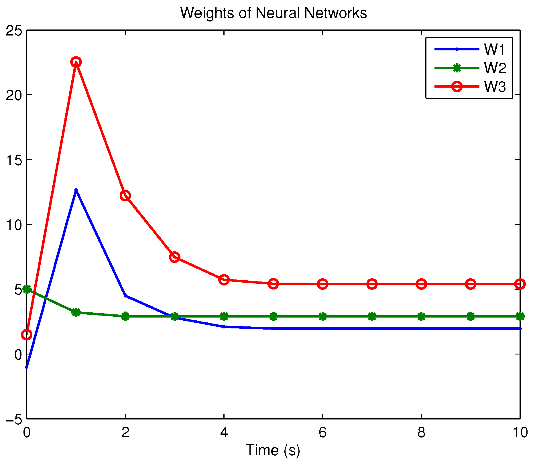
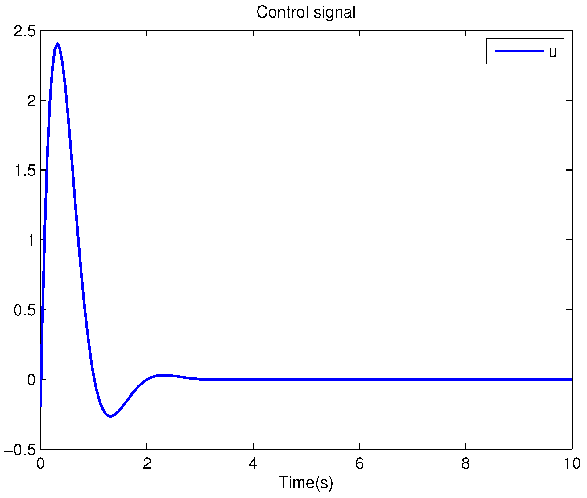
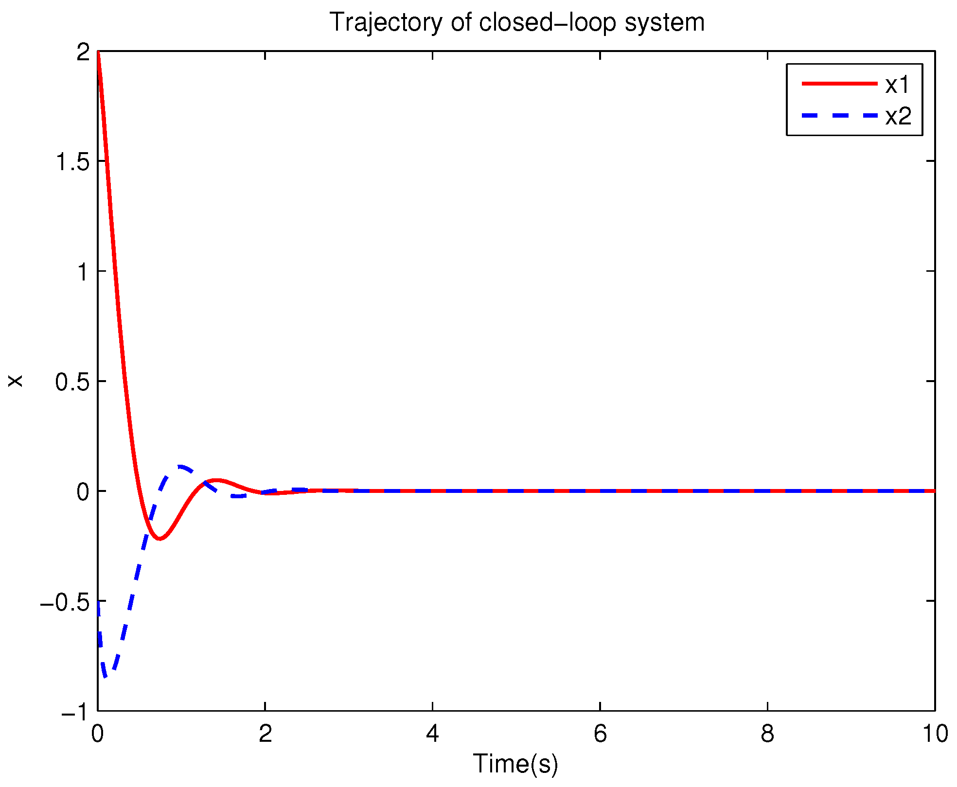
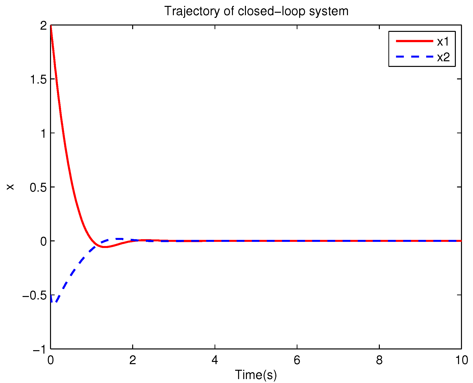
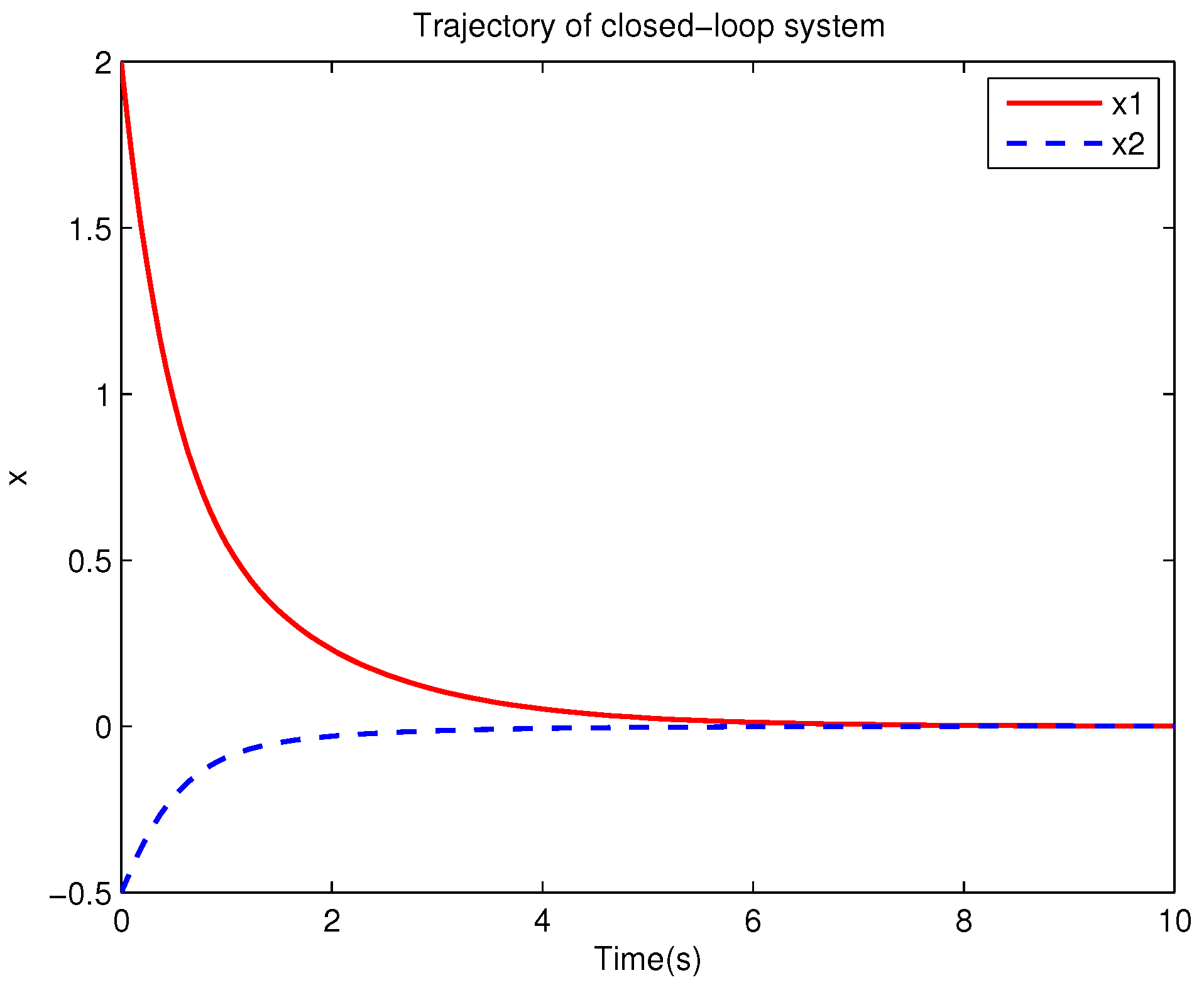
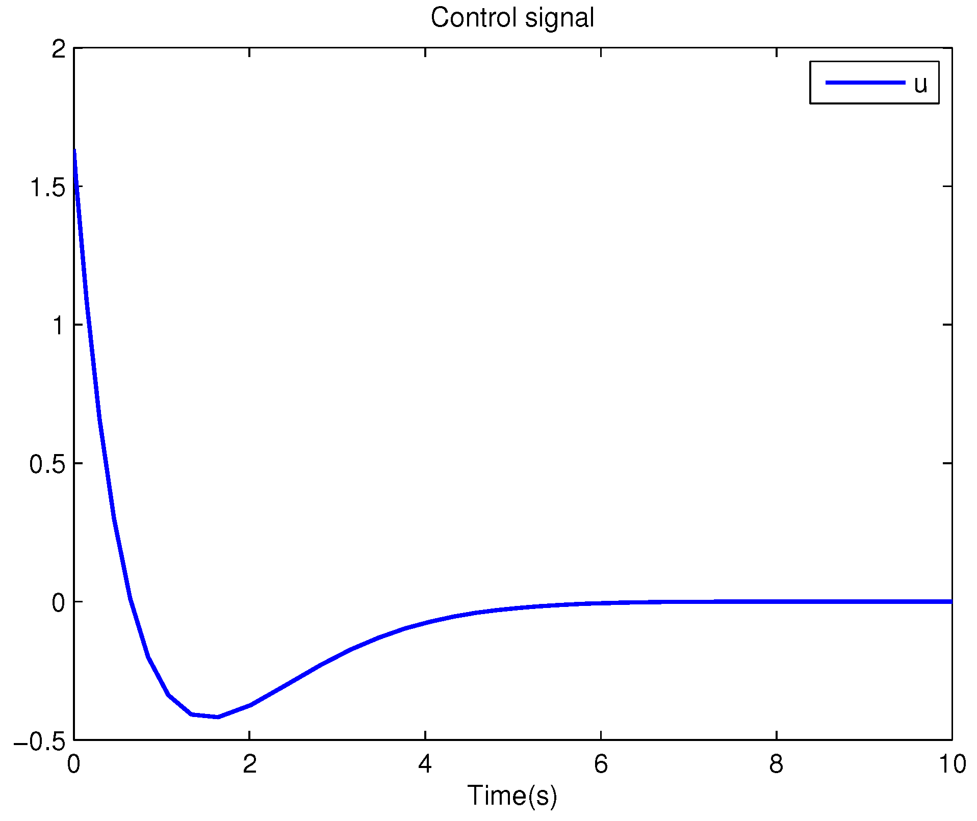
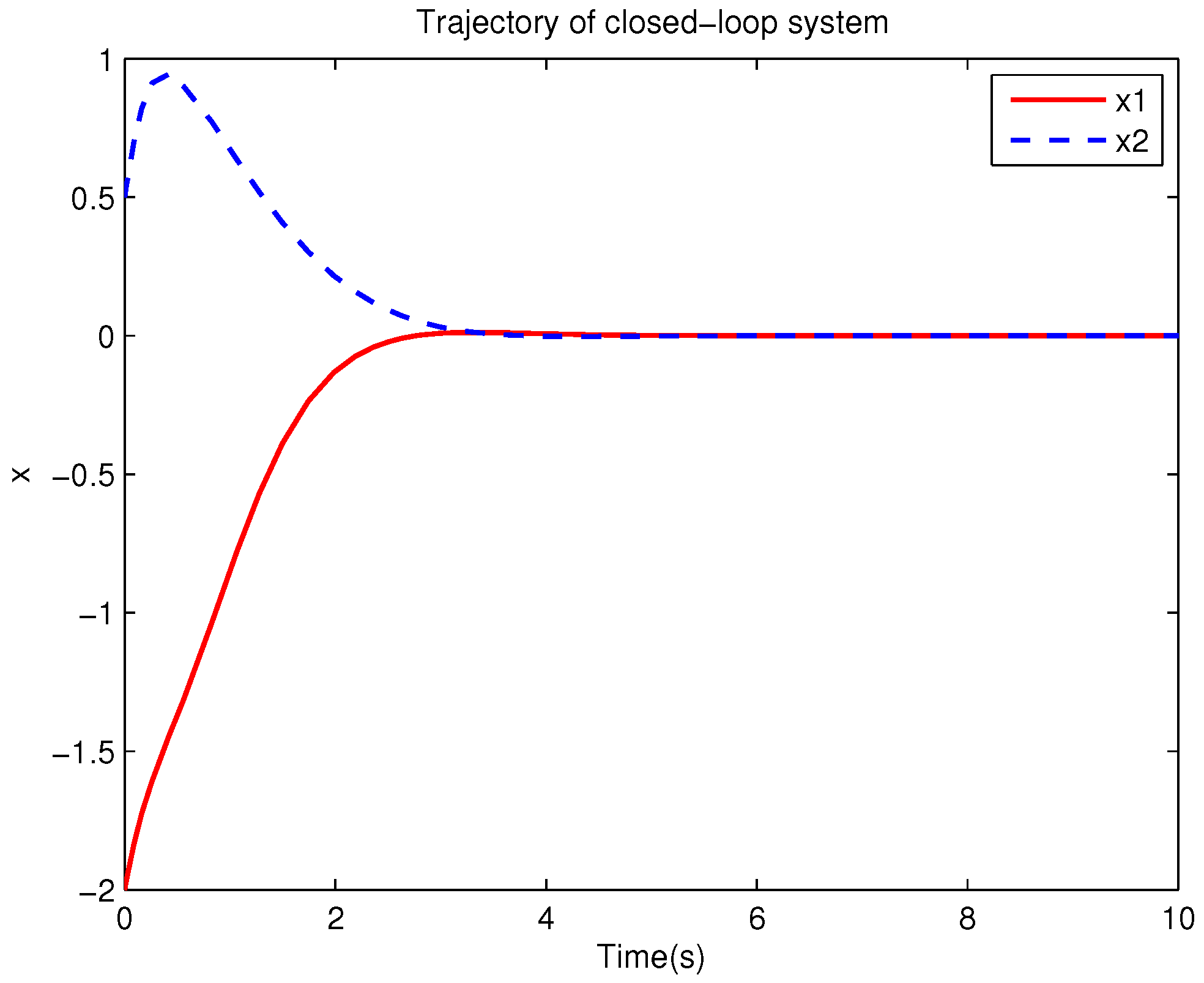
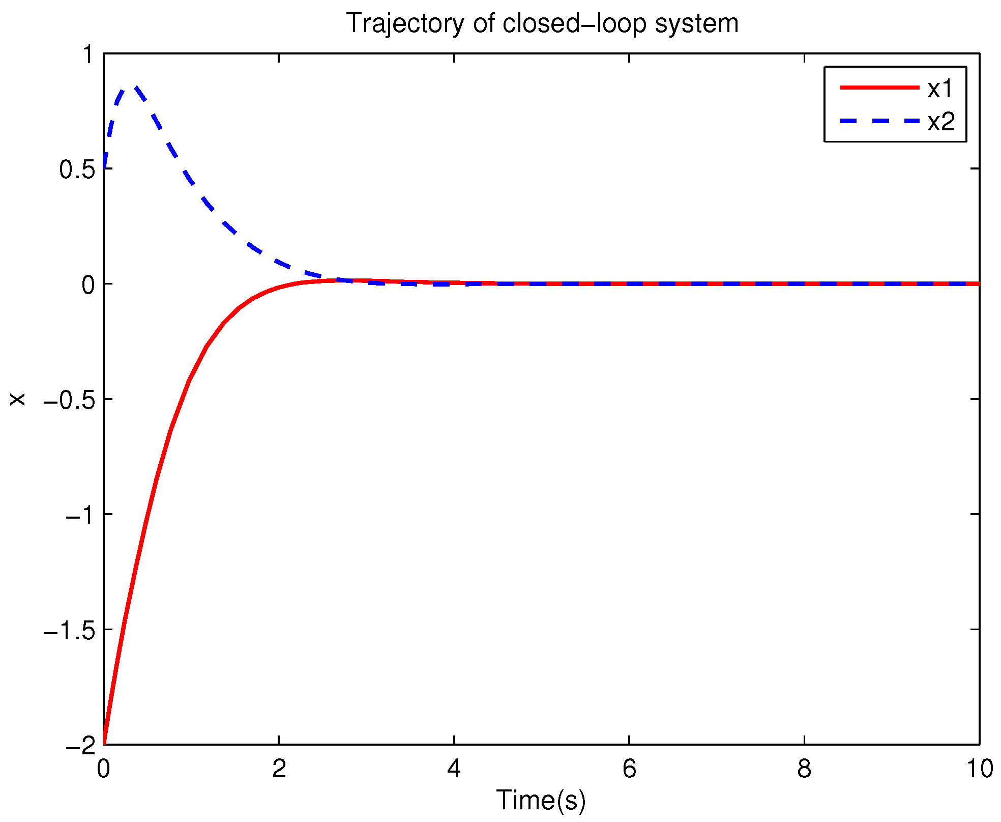
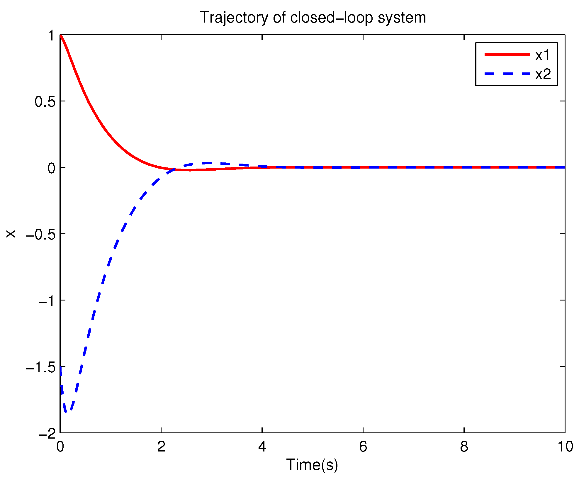
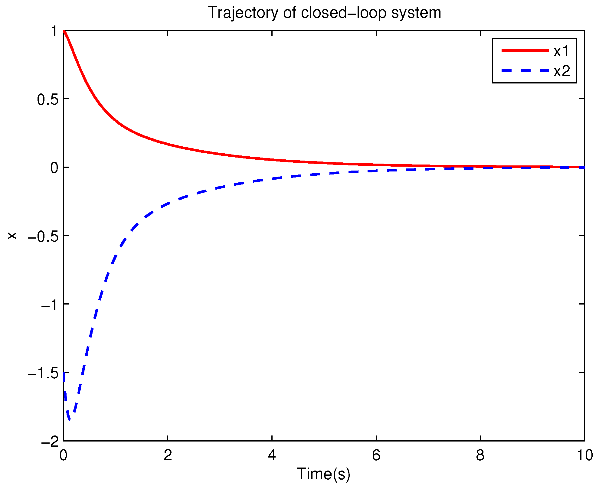
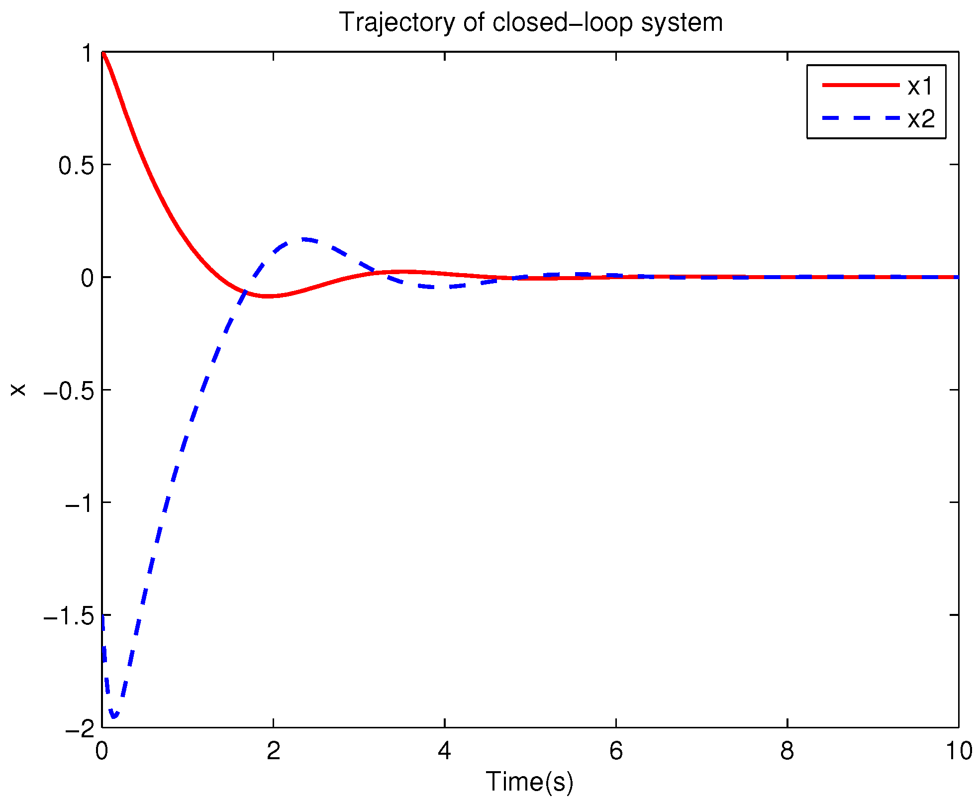
Example 1.

Consider the following uncertain nonlinear systems

$$\dot{x}\left(t\right)=\left[\begin{array}{cc}0& 6\\ -1& 1\end{array}\right]\left[\begin{array}{c}{x}_1\\ x_2\end{array}\right]+\left[\begin{array}{c}0\\ p_1{x}_{1}cos\left(x_2^2\right)\end{array}\right]+\left[\begin{array}{c}0\\ 1+p_2{x}_2^2\end{array}\right]u$$

(47)

where $x={[x_1,x_2]}^T$ is the system state, $\Delta f\left(x\right)=\left[\begin{array}{c}0\\ p_1{x}_{1}cos\left(x_2^2\right)\end{array}\right]$ is the uncertain disturbance function of the system, $\Delta g\left(x\right)=\left[\begin{array}{c}0\\ p_2{x}_2^2\end{array}\right]$ is input uncertainty function, $p_1\in [-2,2]$, $p_2\in [0,10]$.

Obviously,

$$\begin{array}{c}\hfill \Delta f\left(x\right)=g\left(x\right)h\left(x\right),\Delta g\left(x\right)=g\left(x\right)m\left(x\right)\end{array}$$

(48)

where $g\left(x\right)=\left[\begin{array}{c}0\\ 1\end{array}\right]$, $h\left(x\right)=p_1{x}_{1}cos\left(x_2^2\right)$, $m\left(x\right)=p_2{x}_2^2$. Moreover, $\left|h\left(x\right)\right|\le |2x_1|=f_{max}\left(x\right)$. Thus, the original robust control problem is converted into calculating optimal control law. For nominal system

$$\dot{x}\left(t\right)=\left[\begin{array}{cc}0& 6\\ -1& 1\end{array}\right]\left[\begin{array}{c}{x}_1\\ x_2\end{array}\right]+\left[\begin{array}{c}0\\ 1\end{array}\right]u,$$

(49)

find the control function u, such that the performance index

$$\begin{array}{c}\hfill \begin{array}{cc}\hfill J(x,u)& ={\int }_0^{\infty }[f_{max}^2\left(x\right)+x^{T}x+u^{T}u]dt\hfill \\ & ={\int }_0^{\infty }[5x_1^2+x_2^2+u^2]dt\hfill \end{array}\end{array}$$

(50)

is minimized.

In order to solve the robust control problem by using Algorithm 1, it is assumed that the optimal cost function $V^{*}\left(x\right)$ has a neural network structure: $V^{*}\left(x\right)=W^T\varphi \left(x\right)$, where $W={[W_1,W_2,W_3]}^T$, $\varphi \left(x\right)={[x_1^2,x_1{x}_2,x_2^2]}^T$. The initial weight is taken as $W_0={[-1,5,1.5]}^T$, and the initial state of system $x_0={[2,-0.5]}^T$. The neural network weights are calculated iteratively by MATLAB. In each iteration, 10 sets of data samples are collected along the nominal system trajectory to perform the batch least squares problem. After five iterations, the weight converges to $[1.9645,2.8990,5.4038]$. The robust control law of uncertain system (47) is $u^{*}=-1.4495x_1-5.4038x_2$. The convergence process of neural network weight is shown in Figure 1, while the changing process of control signal is shown in Figure 2. The uncertain parameter $p_1$ and $p_2$ in uncertain system (47) take different values, the state trajectories of the closed-loop system are obtained by the robust control law. Figure 3 shows the trajectory of the closed-loop system when $p_1=-2$, $p_2=1$. Figure 4 shows the trajectory of the closed-loop system when $p_1=-1$, $p_2=4$. Figure 5 shows the trajectory of the closed-loop system when $p_1=0$, $p_2=7$. Figure 6 shows the trajectory of the closed-loop system is $p_1=2$, $p_2=10$. From these figures, we can see that the closed-loop system is stable, which shows the effectiveness of the robust control law.

In this example, because of the linear property of the nominal system, MATLAB software can be used to solve LQR problem directly. With this method, the optimal control is calculated as $u^{*}=-1.4496x_1-5.4038x_2$. It is almost the same as the result of neural network approximation, which shows the validity of Algorithm 1.

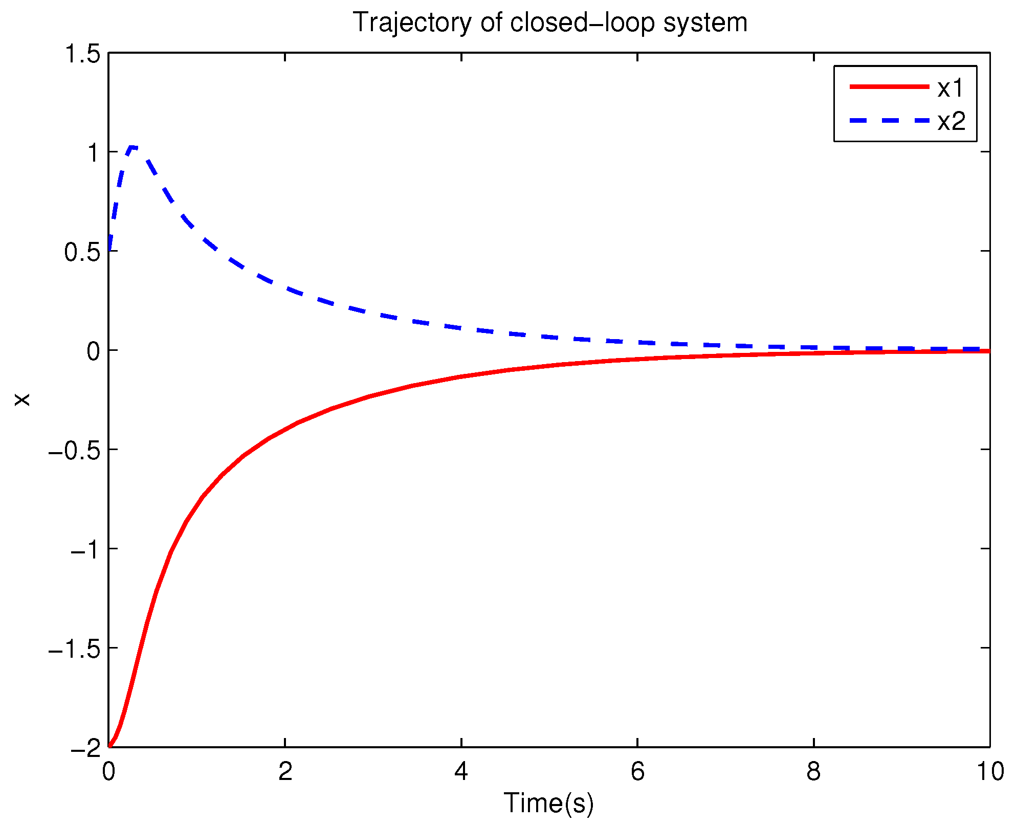
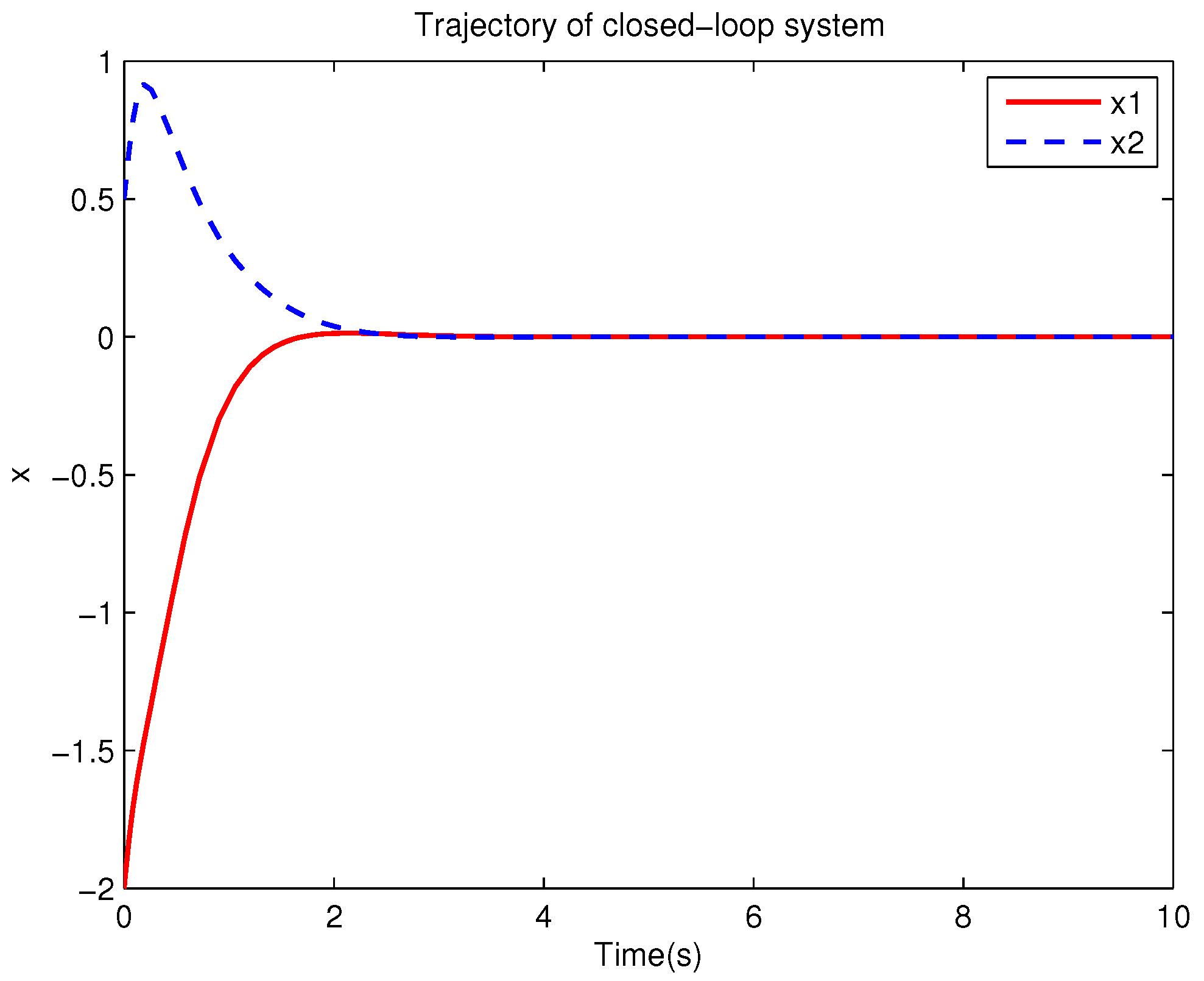
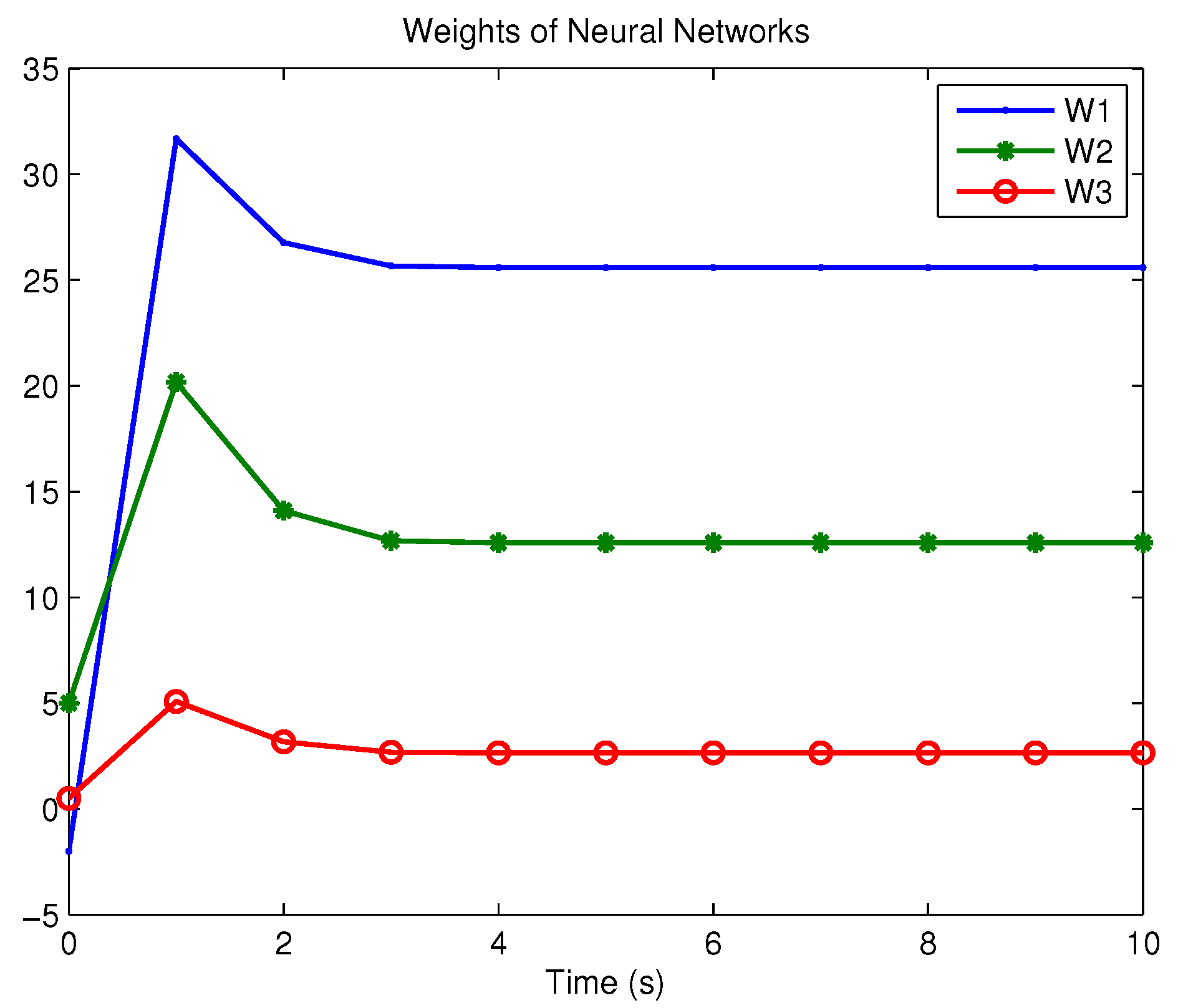
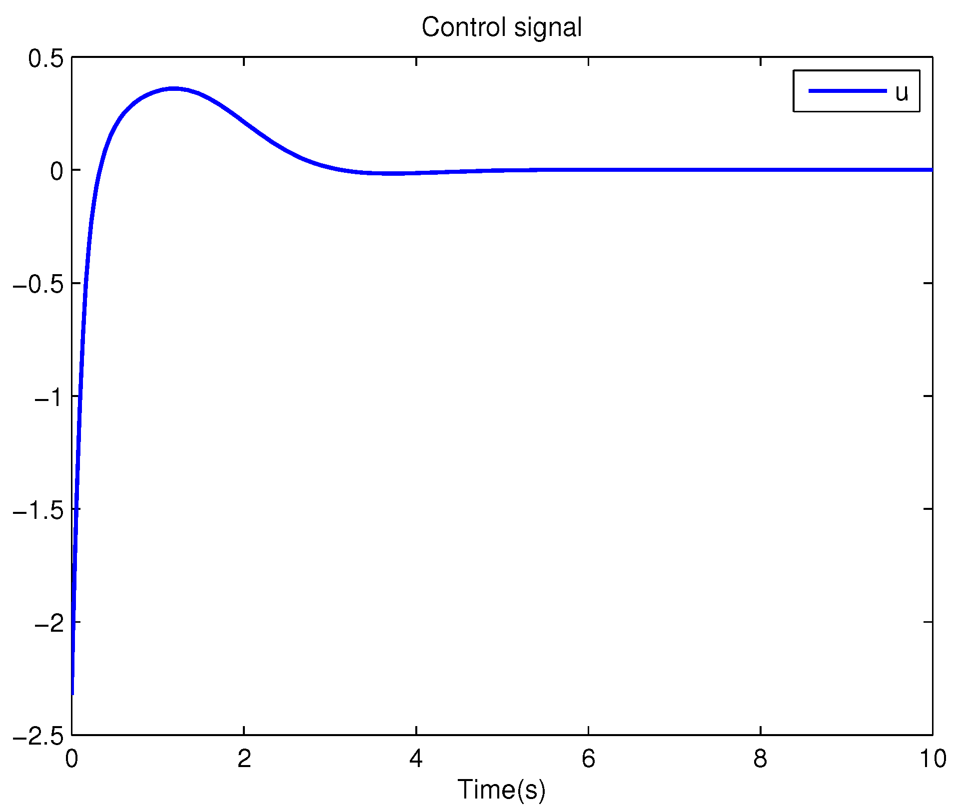
Example 2.

Consider the following uncertain nonlinear systems

$$\dot{x}\left(t\right)=\left[\begin{array}{cc}0& 8\\ -5& 1\end{array}\right]\left[\begin{array}{c}{x}_1\\ x_2\end{array}\right]+\left[\begin{array}{c}0\\ 0.5+p_2{x}_2^2\end{array}\right]u+\left[\begin{array}{c}{p}_1{x}_{1}cos\left(x_2^2\right)+p_3{x}_{2}sin\left(x_1{x}_2\right)\\ 0\end{array}\right]$$

(51)

where $x={[x_1,x_2]}^T$ is the system state, $p_1\in [-2,2]$, $p_2\in [0,5]$, $p_3\in [-1,1]$. Let $\Delta f\left(x\right)=\left[\begin{array}{c}{p}_1{x}_{1}cos\left(x_2^2\right)+p_3{x}_{2}sin\left(x_1{x}_2\right)\\ 0\end{array}\right]$, $\Delta g\left(x\right)=\left[\begin{array}{c}0\\ p_2{x}_2^2\end{array}\right]$. It is easy to know that the system (51) is a mismatched system. The uncertain disturbance of the system is decomposed as

$$\begin{array}{c}\hfill \Delta f\left(x\right)=c\left(x\right)h\left(x\right),\Delta g\left(x\right)=g\left(x\right)m\left(x\right)\end{array}$$

(52)

where, $g\left(x\right)=\left[\begin{array}{c}0\\ 0.5\end{array}\right]$, $c\left(x\right)=\left[\begin{array}{c}1\\ 0\end{array}\right]$, $h\left(x\right)=p_1{x}_{1}cos\left(x_2^2\right)+p_3{x}_{2}sin\left(x_1{x}_2\right)$, $m\left(x\right)=p_2{x}_2^2$. Moreover, $f_{max}\left(x\right)$ and $g_{max}\left(x\right)$ are calculated as follows.

$${\parallel g\left(x\right)}^{+}c\left(x\right)h\left(x\right)\parallel =\parallel \left[\begin{array}{cc}0& 2\end{array}\right]\left[\begin{array}{c}1\\ 0\end{array}\right]h\left(x\right)\parallel =0=f_{max}\left(x\right),$$

and

$$\begin{array}{c}\hfill \begin{array}{c}\hfill \parallel h\left(x\right)\parallel =\parallel p_1{x}_{1}cos\left(x_2^2\right)+p_3{x}_{2}sin\left(x_1{x}_2\right)\parallel \le |2x_1+x_2|=g_{max}\left(x\right)\end{array}\end{array}$$

Select the parameter $\beta =1$. Then the original robust control problem is converted into solving an optimal control problem. For the auxiliary system

$$\dot{x}\left(t\right)=\left[\begin{array}{cc}0& 8\\ -5& 1\end{array}\right]\left[\begin{array}{c}{x}_1\\ x_2\end{array}\right]+\left[\begin{array}{cc}0& 1\\ 0.5& 0\end{array}\right]\overline{u},$$

(53)

find the control policy, $\overline{u}$, such that the following performance index is minimized

$$\begin{array}{cc}\hfill J(x,u)& ={\int }_0^{\infty }[f_{max}^2\left(x\right)+g_{max}^2\left(x\right)+{\beta }^2{x}^{T}x+{\overline{u}}^T\overline{u}]dt\hfill \\ \hfill & ={\int }_0^{\infty }[5x_1^2+2x_2^2+4x_1{x}_2+{\overline{u}}^T\overline{u}]dt.\hfill \end{array}$$

(54)

In order to obtain the obust control law by using Algorithm 2, it is assumed that the optimal cost function $V^{*}\left(x\right)$ has a neural network structure: $V^{*}\left(x\right)=W^T\varphi \left(x\right)$, where $W={[W_1,W_2,W_3]}^T$, $\varphi \left(x\right)={[x_1^2,x_1{x}_2,x_2^2]}^T$. The initial weight is taken as $W_0={[1,-3,0.5]}^T$, and the initial state of system is chosen as $x_0={[-2,0.5]}^T$. The neural network weights are calculated iteratively by MATLAB. In each iteration, 10 sets of data samples are collected along the nominal system trajectory to perform the batch least squares problem. After six iterations, the weight converges to $W={[2.8983,-0.6859,5.2576]}^T$. The optimal control of the auxiliary system is calculated as ${\overline{u}}^{*}=\left[\begin{array}{c}0.1715x_1-2.6288x_2\\ -2.8983x_1+0.3429x_2\end{array}\right]$. The robust control law of the original uncertain system is $u^{*}=0.1715x_1-2.6288x_2$. The convergence process of neural network weight is shown in Figure 7, while the changing process of control signal is shown in Figure 8. The uncertain parameters $p_1$, $p_2$ and $p_3$ in uncertain system (51) take different values, the state trajectories of the closed-loop system are obtained by the robust control law. Figure 9 shows the trajectory of the closed-loop system when $p_1=-1$, $p_2=1$ and $p_3=1$. Figure 10 shows the trajectory of the closed-loop system when $p_1=-1$, $p_2=2$ and $p_3=0$. Figure 11 shows the trajectory of the closed-loop system when $p_1=0.3$, $p_2=3$ and $p_3=-1$. Figure 12 shows the trajectory of the closed-loop system when $p_1=-2$, $p_2=5$ and $p_3=1$. From these figures, we can see that the closed-loop system is stable, which shows the effectiveness of the robust control law.

The nominal system is also a linear system, so MATLAB software can be used to solve LQR problem directly. With this method, the optimal control is calculated as ${\overline{u}}^{*}=\left[\begin{array}{c}0.1713x_1-2.6286x_2\\ -2.8983x_1+0.3430x_2\end{array}\right]$. It has little difference with the approximate result of neural network, which shows the validity of Algorithm 2.

The nominal systems corresponding to the above two examples are linear systems. The following is an example with nonlinear nominal system.

Example 3.

Consider the following uncertain nonlinear systems

$$\dot{x}\left(t\right)=\left[\begin{array}{cc}1& 1\\ -1& -2\end{array}\right]\left[\begin{array}{c}{x}_1\\ x_2\end{array}\right]+\left[\begin{array}{c}0\\ 2x_1^{2}co{s}^2\left(x_2\right)\end{array}\right]+\left[\begin{array}{c}0\\ p_1{x}_{2}co{s}^2\left(x_1\right)\end{array}\right]+\left[\begin{array}{c}0\\ 1+p_2{x}_2^2\end{array}\right]u$$

(55)

where $x={[x_1,x_2]}^T$ is the system state, $\Delta f\left(x\right)=\left[\begin{array}{c}0\\ p_1{x}_{2}co{s}^2\left(x_1\right)\end{array}\right]$ is the uncertain disturbance function of the system, $\Delta g\left(x\right)=\left[\begin{array}{c}0\\ p_2{x}_2^2\end{array}\right]$ is input uncertainty function, $p_1\in [-2,2]$, $p_2\in [0,2]$.

Obviously,

$$\begin{array}{c}\hfill \Delta f\left(x\right)=g\left(x\right)h\left(x\right),\Delta g\left(x\right)=g\left(x\right)m\left(x\right)\end{array}$$

(56)

where $g\left(x\right)=\left[\begin{array}{c}0\\ 1\end{array}\right]$, $h\left(x\right)=p_1{x}_{2}co{s}^2\left(x_1\right)$, $m\left(x\right)=p_2{x}_2^2$. Moreover, $\left|h\left(x\right)\right|\le |2x_2|=f_{max}\left(x\right)$. Thus, the original robust control problem is converted into calculating optimal control law. For nominal system

$$\dot{x}\left(t\right)=\left[\begin{array}{cc}1& 1\\ -1& -2\end{array}\right]\left[\begin{array}{c}{x}_1\\ x_2\end{array}\right]+\left[\begin{array}{c}0\\ 2x_1^{2}co{s}^2\left(x_2\right)\end{array}\right]+\left[\begin{array}{c}0\\ 1\end{array}\right]u,$$

(57)

find the control function u, such that the performance index

$$\begin{array}{c}\hfill \begin{array}{cc}\hfill J(x,u)& ={\int }_0^{\infty }[f_{max}^2\left(x\right)+x^{T}x+u^{T}u]dt\hfill \\ & ={\int }_0^{\infty }[x_1^2+5x_2^2+u^2]dt\hfill \end{array}\end{array}$$

(58)

is minimized.

In order to solve the robust control problem by using Algorithm 1, it is assumed that the optimal cost function $V^{*}\left(x\right)$ has a neural network structure: $V^{*}\left(x\right)=W^T\varphi \left(x\right)$, where $W={[W_1,W_2,W_3]}^T$, $\varphi \left(x\right)={[x_1^2,x_1{x}_2,x_2^2]}^T$. The initial weight is taken as $W_0={[-2,5,0.5]}^T$, and the initial state of system $x_0={[2,-0.5]}^T$. The neural network weights are calculated iteratively by MATLAB. In each iteration, 10 sets of data samples are collected along the nominal system trajectory to perform the batch least squares problem. After five iterations, the weight converges to $[25.5830,12.5830,2.6458]$. The robust control law of uncertain system (55) is $u^{*}=-6.2915x_1-2.6458x_2$. The convergence process of neural network weight is shown in Figure 13, while the changing process of control signal is shown in Figure 14. The uncertain parameter $p_1$ and $p_2$ in uncertain system (55) take different values, the state trajectories of the closed-loop system are obtained by the robust control law. Figure 15 shows the trajectory of the closed-loop system when $p_1=1$, $p_2=0.8$. Figure 16 shows the trajectory of the closed-loop system when $p_1=-0.5$, $p_2=1$. Figure 17 shows the trajectory of the closed-loop system when $p_1=1$, $p_2=2$. Figure 18 shows the trajectory of the closed-loop system is $p_1=2$, $p_2=1$. From these figures, we can see that the closed-loop system is stable, which shows the effectiveness of the robust control law.

7. Conclusions

In this paper, the PI algorithms in RL are proposed to solve robust control problem for a class of nonlinear continuous time uncertain system. The robust control law is obtained without knowing the internal dynamics of the nominal system. The considered robust control problem is converted into solving an optimal control problem containing a nominal or auxiliary system with a predefined performance index. The online PI algorithms are established to calculate the robust controller of matched and mismatched system. The numerical examples are given to show the availability of the theoretical results. The proposed method may be extended to solve robust tracking problems for some nonlinear systems with uncertainty entering output, which may be the subject of our future research.