Matching Point Clouds with STL Models by Using the Principle Component Analysis and a Decomposition into Geometric Primitives

Abstract

While repairing industrial machines or vehicles, recognition of components is a critical and time-consuming task for a human. In this paper, we propose to automatize this task. We start with a Principal Component Analysis (PCA), which fits the scanned point cloud with an ellipsoid by computing the eigenvalues and eigenvectors of a 3-by-3 covariant matrix. In case there is a dominant eigenvalue, the point cloud is decomposed into two clusters to which the PCA is applied recursively. In case the matching is not unique, we continue to distinguish among several candidates. We decompose the point cloud into planar and cylindrical primitives and assign mutual features such as distance or angle to them. Finally, we refine the matching by comparing the matrices of mutual features of the primitives. This is a more computationally demanding but very robust method. We demonstrate the efficiency and robustness of the proposed methodology on a collection of 29 real scans and a database of 389 STL (Standard Triangle Language) models. As many as 27 scans are uniquely matched to their counterparts from the database, while in the remaining two cases, there is only one additional candidate besides the correct model. The overall computational time is about 10 min in MATLAB.

1. Introduction

Computer recognition of 3-dimensional (3D) objects is of a high interest in all domains where the identification of an a priori unknown object is required, e.g., when repairing a complex machine that consists of thousands of mechanical components. A typical problem that arises is matching a component, possibly damaged, to its drawing, nowadays an STL (Standard Triangle Language) triangulation. For a human, this is a demanding task. Fortunately, the human can be replaced with a robotical system, which scans the surface of the component and matches the resulting point cloud with a unique item from the database of STL triangulations of the mechanical components. The aim of this paper is to provide a fast and robust computational method for this matching.

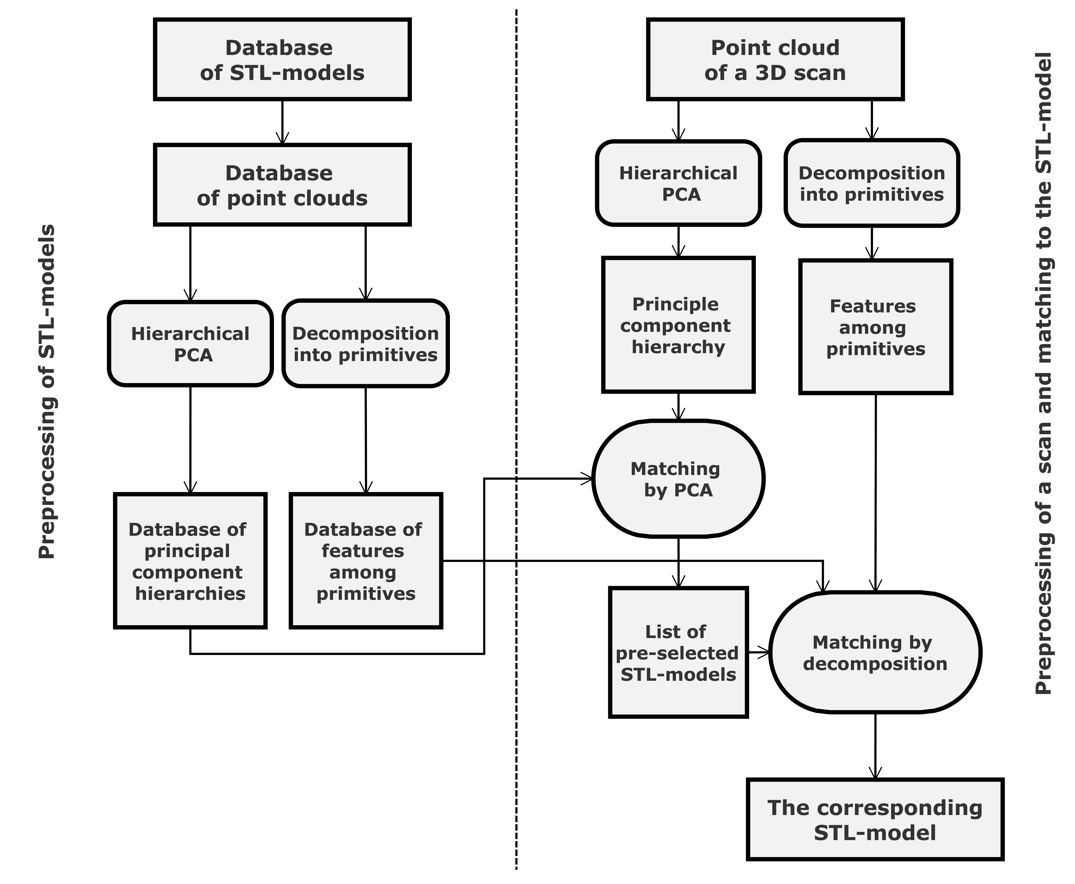
We propose the successive use of two methods. The first one relies on the Principal Component Analysis (PCA), which is fast. However, it may not result in a unique match but rather in a small collection of candidates. Therefore, we developed yet another method that relies on decomposition into planar and cylindrical primitives. This is robust, meaning that it typically results in a unique match. This method exhibits a higher computational complexity, which is not critical, so we apply it to the small collection of models preselected by the first method. The overall scheme of our methodology is depicted in Figure 1.

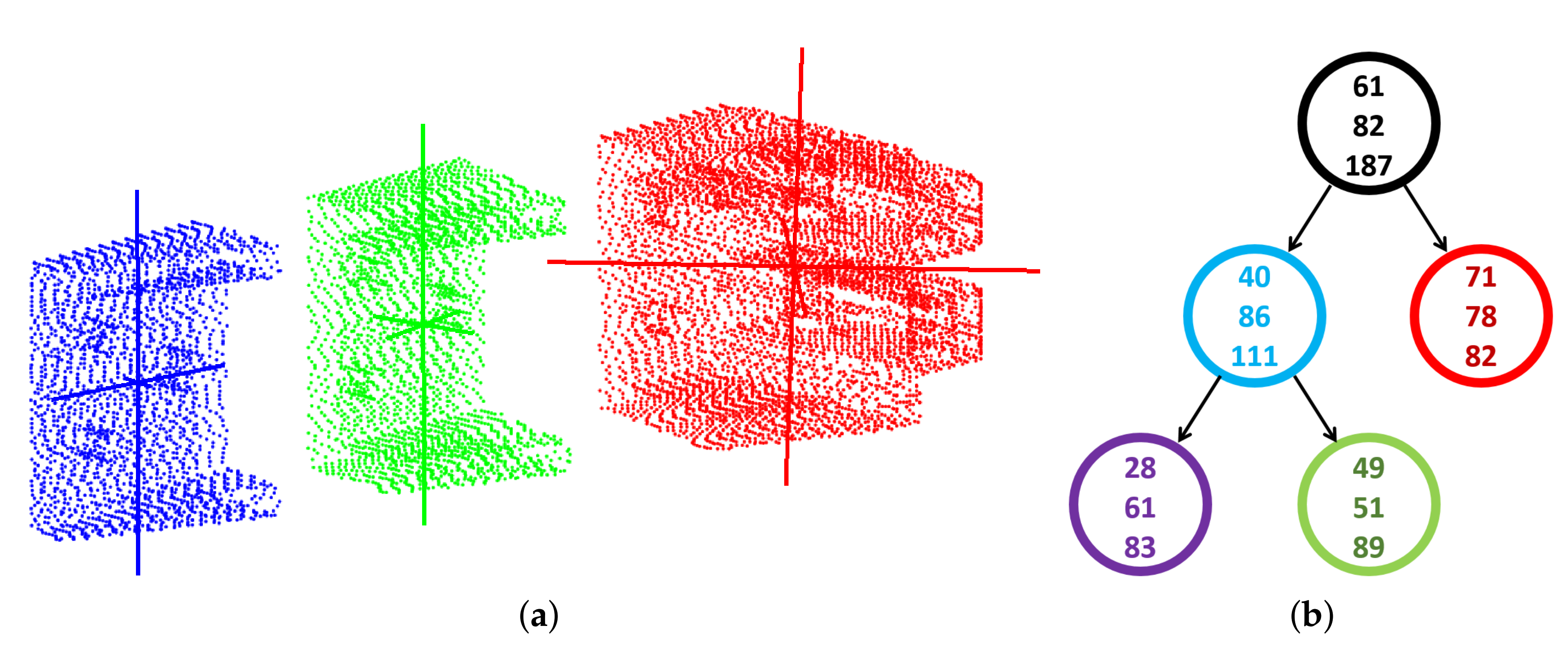
Principal Component Analysis (PCA) fits the point cloud with an ellipsoid by means of computing the eigenvalues and eigenvectors of a 3-by-3 covariant matrix. In case there is a dominant eigenvalue, the point cloud is decomposed into two clusters to which the PCA is applied recursively. This results in a binary tree, where each vertex (corresponding to a cluster of points) is associated with the three eigenvalues. The algorithm is also applied (preprocessing phase) to all the STL triangulations from the database. The matching is performed by comparing the trees and the triples of eigenvalues. This algorithm has an almost linear complexity with respect to the number of points and a logarithmic complexity with respect to the number of STL triangulations in the database. Hence, on a single processor, it is an optimal complexity method. A drawback is that the method fails in cases with objects differing by small details. The result of the PCA is a small collection of STL triangulations.

To overcome the lack of robustness of the PCA, we developed another method. It exploits the fact that surfaces of mechanical parts are mostly planar or cylindrical. We decomposed each object in the database (preprocessing phase) as well as the scan into planar and cylindrical primitives. For each STL triangulation and the point cloud, we computed four matrices—two for planar and the other two for cylindrical primitives. One of the two contains distances, and the other one contains angles between the primitives. The construction of such matrices has a quadratic computational complexity with respect to the number of points or triangles. Finally, we evaluate the similarity of the matrices of the point cloud to the respective matrices of STL triangulations. This has an unpleasant combinatorial complexity with respect to the number of primitives; hence, it is crucial that we apply this method to the small collection of objects preselected by PCA.

2. Related Work

The method PCA has been a well-known concept for a century [1]. Although it was discovered in the context of statistical analysis [2], it is applicable in many modern areas of research. We refer to [3], which focuses on machine learning. The PCA also has good application for sparsification of densely populated matrices arising in boundary element methods [4,5].

Decomposition of point clouds into geometrical primitives relies on the RANSAC (Random Sample Consensus) algorithm [6]. It chooses random points from the point cloud and tries to form them into planes cylinders, spheres, cones, or tori. Note that the key features of the algorithm that we use include estimation of normals [7], detection of planes [8], and detection of cylinders [9]. The algorithm is fast also due to exploitation of oct-tree sampling. In [10], the authors processed topology graphs on top of the geometric primitives, labelled the vertices and edges with features, and finally matched the point clouds with the given shapes. They applied the method in the architectural domain. This paper is the main inspiration for our second method. Similarly, we are inspired by [11], where the authors additionaly reconstructed incomplete point clouds. This is exactly what we do when a mechanical component to be recognized is damaged. In [12], the authors extended their method and its use in architecture by allowing measurements of wall thickness, for instance. Another interesting approach is template matching [13], where the authors do not extract features but rather search for templates in the point cloud.

Various combinations of PCA and the RANSAC algorithm have appeared mostly in geoscience research. In [14] the authors evaluated hierarchical point cluster correlations, which are in a sense similar to hierarchical PCA, and they applied sparse coding to identify complex geometries. Another very similar approach to ours is described in [15], where a locally affine-invariant geometric constraint effectively handles processing of point clouds. In [16], contour areas of building facades were extracted and the objects were identified using PCA and finalized with RANSAC to identify planes. Another hierarchical approach using oct-trees was considered in [17] for a lossy compression of static point clouds.

There is an important direction relying on optimization methods. In [18], the authors employed least-square fitting of 6 rigid body modes to recognize objects under affine transformations. This has actually been suggested in the scholarly paper of [19]. In [20], it wsa observed that the metrics to be minimized have many local minimizers and that searching for the global minimum is of utmost importance. A very interesting new approach was suggested in [21], where the authors employed an L1-metric (integral from the function absolute value) and linear programming, where the search set was successively convexified.

Many methods rely on statistics. In [22], the authors considered point histogram features. Similarly, in [23], a comparison of histograms of pairwise diffusion distances and histograms of pairwise geodesic distances was made.

Novel techniques for representations of objects have also been proposed. In [24], 3D wireframes were revisited to be adjusted relative 3D positions of object parts. In [25], 3D shapes were matched to polyhedral objects by comparing multiresolution graphs, which are typically geodesic distance functions.

Finally, as computational power is nowadays great, a large amount of work on object recognition has been devoted to artificial intelligence techniques such as deep neural networks [26] or support vector machines.

3. Principal Component Analysis

We consider a cloud $C=\{P_1,P_2,\dots ,P_N\}\subset {\mathbb{R}}^3$ of N 3D points. We compute the mass point $P\in {\mathbb{R}}^3$ and the covariant matrix $M\in {\mathbb{R}}^{3\times 3}$,

$$P=\frac{1}{N}\sum _{i=1}^N{P}_i,M_{jk}=\frac{1}{N}\sum _{i=1}^N{(P_i-P)}_j{(P_i-T)}_k.$$

Since M is real-valued, symmetric, and positive definite, it has three positive eigenvalues,

$$0<{\lambda }_3\le {\lambda }_2\le {\lambda }_1$$

and the related eigenvectors can be formed into an orthonormal system $(v_1,v_2,v_3)$, i.e., $v_i·v_j={\delta }_{ij}$, where ${\delta }_{ij}$ is the Dirac delta function. In fact, the vectors

$${\tilde{\lambda }}_1{v}_1,{\tilde{\lambda }}_2{v}_2,{\tilde{\lambda }}_3{v}_3,\mathrm{where}{\tilde{\lambda }}_i=2\sqrt{{\lambda }_i},$$

(1)

form semi-axes of in a sense best-fitted ellipsoid; see Figure 2.

Notice that (1) is motivated by the fact that ${\lambda }_i$, $i=1,2,3$, are eigenvalues of the covariant matrix of the ellipsoidal point cloud of $N=N_1\times N_2$ points

$$P_{\mathbf{i}}=\left(\begin{array}{c}{\tilde{\lambda }}_{1}sin{\theta }_{i_1}cos{\phi }_{i_2}\\ {\tilde{\lambda }}_{2}sin{\theta }_{i_1}sin{\phi }_{i_2}\\ {\tilde{\lambda }}_{3}cos{\theta }_{i_1}\end{array}\right),$$

where $\mathbf{i}=(i_1,i_2)$ is a multi-index; ${\theta }_{i_1}=\frac{i_1}{N_1}\pi$, $i_1=1,2,\cdots ,N_1$; and ${\phi }_{i_2}=\frac{i_2}{N_2}2\pi$, $i_2=1,2,\cdots ,N_2$. For completeness, we recall that the eigenvalues are computed by Kardan’s formulae:

$$\left\{{\lambda }_1,{\lambda }_2,{\lambda }_3\right\}=\left\{2rcos\frac{\varphi }{3}-\frac{a}{3},-2rcos\frac{\varphi \pm \pi }{3}-\frac{a}{3}\right\},$$

where $\varphi =arccos\left(-\frac{q}{2r^3}\right)$; $r=-\frac{1}{3}\sqrt{|-a^2+3b|}$; $q=-\frac{2a^3}{27}+\frac{ab}{3}-c$; and $a=\mathrm{tr}M=M_{11}+M_{22}+M_{33}={\lambda }_1+{\lambda }_2+{\lambda }_3$, $b=\frac{1}{2}({\left(\mathrm{tr}M\right)}^2-\mathrm{tr}{M}^2)={\lambda }_1{\lambda }_2+{\lambda }_1{\lambda }_3+{\lambda }_2{\lambda }_3$, and $c=\det M={\lambda }_1{\lambda }_2{\lambda }_3$ are the three principle matrix invariants.

In the case of a dominant axis, $(1-\epsilon ){\tilde{\lambda }}_1>{\tilde{\lambda }}_2$, where $\epsilon \in (0,1)$ is a relative tolerance, we divide the point cloud C into sub-clouds $C_1$ and $C_2$ by a cutting plane, which has the normal direction $v_1$ and contains the following mass point:

$$C_1=\left\{P_i\in C:(P_i-P)·v_1\ge 0\right\},C_2=C\backslash C_1.$$

We apply PCA recursively to $C_1$ and $C_2$; see Figure 3. This way, we proceed and construct a subdivision binary tree. The vertices of the tree are associated with the length of the ellipsoid semi-axes (1). The leaves satisfy ${\tilde{\lambda }}_1\approx {\tilde{\lambda }}_2$ and represent objects such as balls or squab cylinders. In Figure 4, we depict a subdivision of a point cloud and the related tree.

Matching Point Clouds Using PCA

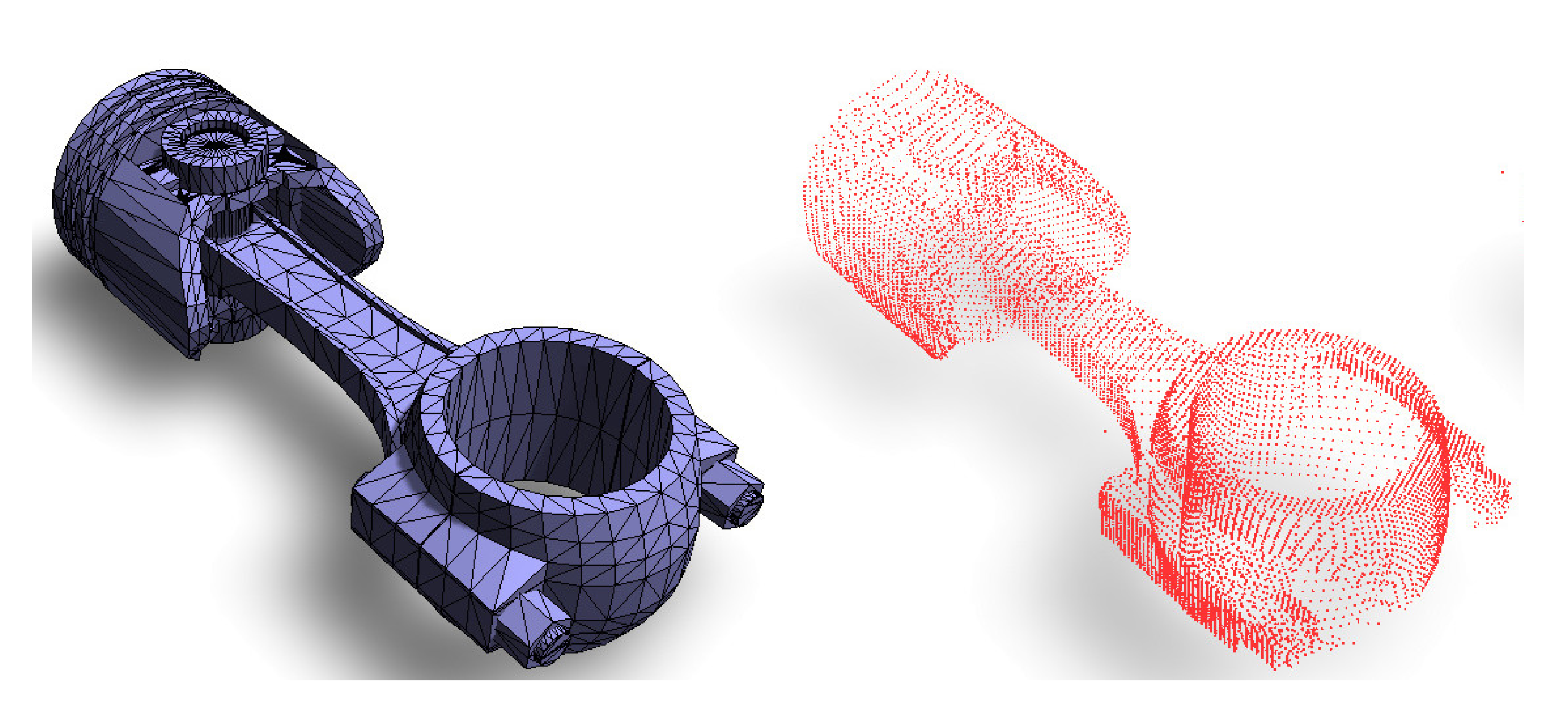
First, the recursive PCA is applied to each of the STL triangulations from the database of models. Each triangle is covered with points with as equal as possible surface density. We then apply the PCA to this auxiliary point cloud and store the resulting tree in the database. Moreover, access to the database can be significantly accelerated by indexing the database according to the semi-axis lengths of the ellipsoids associated with the root vertices of the trees.

The matching of a scanned point cloud to STL triangulations proceeds as follows: For the scanned point cloud, we compute its three semi-axis lengths and find candidates from the database with the same triples up to the tolerance $\epsilon$. The measure is the standard 3D Euclidean norm:

$$∥\tilde{\lambda }-\tilde{\xi }∥<\epsilon ∥\tilde{\lambda }∥,∥\tilde{\lambda }∥=\sqrt{{({\tilde{\lambda }}_1)}^2+{({\tilde{\lambda }}_2)}^2+{({\tilde{\lambda }}_3)}^2},$$

(2)

where $\tilde{\lambda }=\left({\tilde{\lambda }}_1,{\tilde{\lambda }}_2,{\tilde{\lambda }}_3\right)$ and $\tilde{\xi }=\left({\tilde{\xi }}_1,{\tilde{\xi }}_2,{\tilde{\xi }}_3\right)$ are the ellipsoidal semi-axis lengths of the scanned point cloud and of a point cloud from the database, respectively. If there is no unique candidate at this zero level, we repeat the matching procedure at the first level of the trees, provided that it is applicable at least to the tree of the scanned point cloud. For all admissible first-level candidates, we apply (2) to the two sons of the root vertex and use the 6D Euclidean norm, i.e., $\parallel \mathbf{v}\parallel =\sqrt{{\sum }_{i=1}^6{\left(v_i\right)}^2}$, as the measure. If necessarry, we proceed to the next level (in the case of two or four second-level sons) and so on.

4. Decomposition into Geometric Primitives

While we implemented the previous method from scratch, in this second method, we relied on the open-source software package Point Cloud Library (PCL) [27,28]. For each point cloud, either the scan or the auxiliary point cloud were created from an STL triangulation; we proceed with three major steps:

• Identify geometrical primitives that are sub-clouds of points belonging to the same plane or cylinder.
• Calculate the following four pairwise-feature matrices: distances between the parallel planar primitives, angles between the planar primitives, distances between the parallel axes of the cylindrical primitives, and angles between the axes of the cylindrical primitives.
• Find the STL triangulation of the feature matrices that fits best with the feature matrices of the scanned point cloud.

Now, we present the details of the procedures behind these three steps.

4.1. Identification of Geometrical Primitives

Given a point cloud C, we find the largest planar sub-cloud using the PCL command pcfitplane, that results in a sub-cloud $C^{\mathrm{pl}}$ and the plane equation

$$n·x+d=0,x=(x_1,x_2,x_3)\in {\mathbb{R}}^3,$$

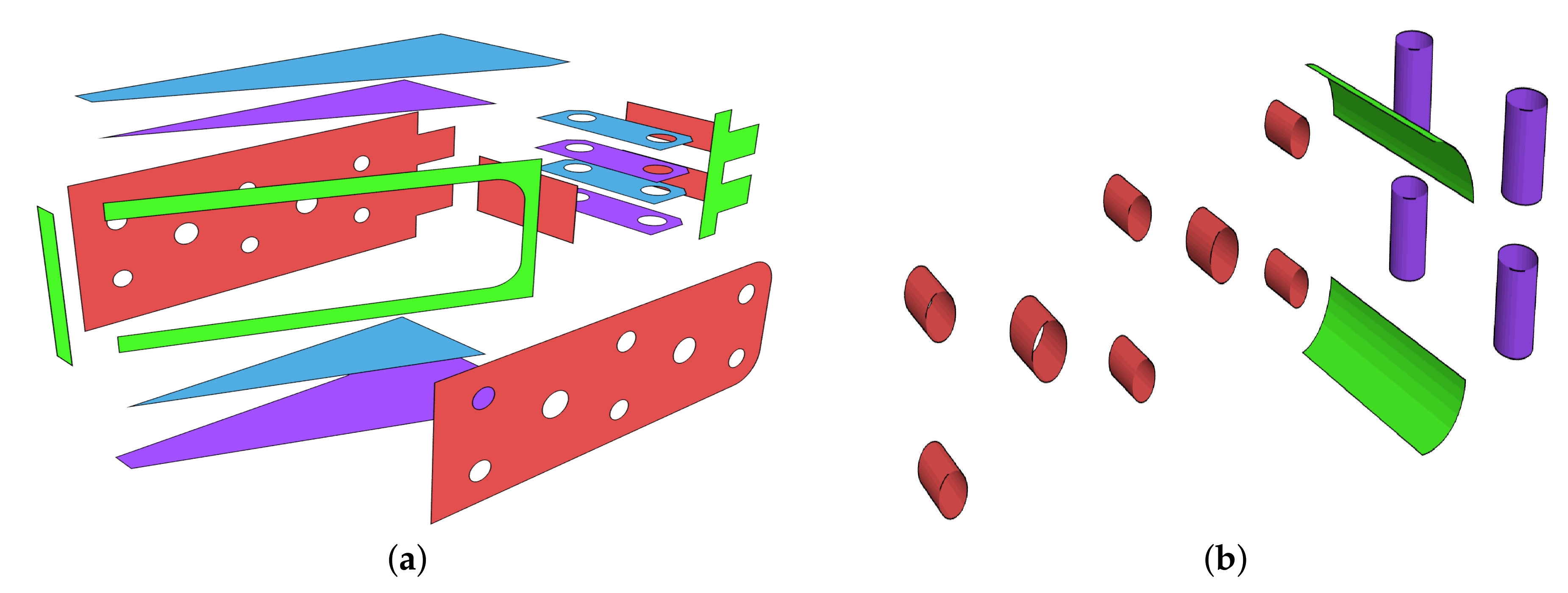
where $n\in {\mathbb{R}}^3$ is the unit ($\parallel n\parallel =1$) normal direction and $d\in \mathbb{R}$. In Figure 5, we depict the decomposition of an object into planar primitives.

Next, we subtract the sub-cloud $C=C\backslash C^{\mathrm{pl}}$ and find the largest cylindrical subcloud using the PCL command, pcfitcylinder, that results in a sub-cloud $C^{\mathrm{cyl}}$ and the cylinder equation

$${\parallel x-P\parallel }^2=r^2+{\left[(x-P)·(Q-P)\right]}^2,$$

where $P=(P_1,P_2,P_3)\in {\mathbb{R}}^3$ and $Q=(Q_1,Q_2,Q_3)\in {\mathbb{R}}^3$ are two distinct points on the cylinder axis and $r>0$ is the radius. In Figure 5, we depict the cylindrical primitives.

We subtract the sub-cloud $C=C\backslash C^{\mathrm{cyl}}$ and repeat the procedure to find the second largest planar and cylindrical primitives until the PCL commands fail or the number of points in the sub-cloud is below our tolerance. We arrive at $N^{\mathrm{pl}}$ planar sub-clouds:

$$C_1^{\mathrm{pl}},C_2^{\mathrm{pl}},\cdots ,C_{N^{\mathrm{pl}}}^{\mathrm{pl}},$$

(3)

each of which, $C_i^{\mathrm{pl}}$, is associated with the normal vector $n_i^{\mathrm{pl}}\in {\mathbb{R}}^3$ and the shift $d_i^{\mathrm{pl}}\in \mathbb{R}$. Furthermore, this results in $N^{\mathrm{cyl}}$ cylindrical sub-clouds:

$$C_1^{\mathrm{cyl}},C_2^{\mathrm{cyl}},\cdots ,C_{N^{\mathrm{cyl}}}^{\mathrm{cyl}},$$

(4)

each of which, $C_i^{\mathrm{cyl}}$, is associated with the points $P_i^{\mathrm{cyl}},Q_i^{\mathrm{cyl}}\in {\mathbb{R}}^3$ determining the axis and the radius $r_i^{\mathrm{cyl}}>0$. Note that the order of the sub-clouds matters as larger sub-clouds were likely identified by the PCL commands earlier.

4.2. Pairwise-Feature Matrices

Consider a point cloud C and the decomposition into $N^{\mathrm{pl}}$ planar primitives (3). We compute the following two matrices of pairwise distances and angles:

$$D^{\mathrm{pl}}\in {\mathbb{R}}_{+}^{N^{\mathrm{pl}}\times N^{\mathrm{pl}}},A^{\mathrm{pl}}\in {[0,\pi /2]}^{N^{\mathrm{pl}}\times N^{\mathrm{pl}}},$$

where

$$A_{ij}^{\mathrm{pl}}=arccos\left|n_i^{\mathrm{pl}}·n_j^{\mathrm{pl}}\right|,$$

$$D_{ij}^{\mathrm{pl}}=\left\{\begin{array}{cc}0,\hfill & A_{ij}^{\mathrm{pl}}<\mathrm{tolerance},\hfill \\ |d_i^{\mathrm{pl}}-d_j^{\mathrm{pl}}|,\hfill & \mathrm{otherwise}.\hfill \end{array}\right.$$

Similarly, we compute the two matrices of pairwise distances and angles between the axes of the $N^{\mathrm{cyl}}$ cylindrical primitives (4):

$$D^{\mathrm{cyl}}\in {\mathbb{R}}_{+}^{N^{\mathrm{cyl}}\times N^{\mathrm{cyl}}},A^{\mathrm{cyl}}\in {[0,\pi /2]}^{N^{\mathrm{cyl}}\times N^{\mathrm{cyl}}},$$

where

$$A_{ij}^{\mathrm{cyl}}=arccos\left|v_i^{\mathrm{cyl}}·v_j^{\mathrm{cyl}}\right|,$$

$$D_{ij}^{\mathrm{cyl}}=\left\{\begin{array}{cc}0,\hfill & A_{ij}^{\mathrm{cyl}}<\mathrm{tolerance},\hfill \\ \left|(P_j^{\mathrm{cyl}}-P_i^{\mathrm{cyl}})·(v_i^{\mathrm{cyl}}\times v_j^{\mathrm{cyl}})\right|,\hfill & \mathrm{otherwise},\hfill \end{array}\right.$$

where $v_i^{\mathrm{cyl}}=\frac{1}{∥Q_i^{\mathrm{cyl}}-P_i^{\mathrm{cyl}}∥}(Q_i^{\mathrm{cyl}}-P_i^{\mathrm{cyl}})\in {\mathbb{R}}^3$ is the unit axial direction.

4.3. Matching Procedure

Matching of the point cloud of a scan with the auxiliary point cloud of an STL triangulation is done by finding the number of geometric primitives that are common to the scan and to the STL model. Unfortunately, calculating this number is computationally demanding. Namely, it has a combinatorial complexity as it needs to find proper permutations of the pairwise-feature matrices.

Consider the plane-distance matrices $D^{\mathrm{pl},\mathrm{scan}}$ and $D^{\mathrm{pl},\mathrm{model}}$ of the scan and the model, respectively, and the related plane-angle matrices $A^{\mathrm{pl},\mathrm{scan}}$ and $A^{\mathrm{pl},\mathrm{model}}$. We take sorted nonzero entries of the first column of $D^{\mathrm{pl},\mathrm{scan}}$ and the first column of $A^{\mathrm{pl},\mathrm{scan}}$. We look for the column index in $D^{\mathrm{pl},\mathrm{model}}$ and $A^{\mathrm{pl},\mathrm{model}}$ such that the columns are the same up to a tolerance. In case where we succeed, we find the first common planar primitive; we remove the affected rows and columns from $D^{\mathrm{pl},\mathrm{scan}}$, $A^{\mathrm{pl},\mathrm{scan}}$, $D^{\mathrm{pl},\mathrm{model}}$, and $A^{\mathrm{pl},\mathrm{model}}$; and we continue to search for the second common planar primitive. In cases where we fail, we remove the first column from $D^{\mathrm{pl},\mathrm{scan}}$ and from $A^{\mathrm{pl},\mathrm{scan}}$ and repeat the procedure with the next (originally second) column of $D^{\mathrm{pl},\mathrm{scan}}$ and $A^{\mathrm{pl},\mathrm{scan}}$. This way, we proceed until we remove all the columns from either matrix. Finally, we repeat the procedure for the cylindrical feature matrices $D^{\mathrm{cyl},\mathrm{scan}}$, $A^{\mathrm{cyl},\mathrm{scan}}$, $D^{\mathrm{cyl},\mathrm{model}}$, and $A^{\mathrm{cyl},\mathrm{model}}$ and add the number of common cylindrical primitives to the number of common planar primitives. We store this total number of common primitives.

The procedure is performed for all models from the database. The model with the maximal number of common primitives is recognized as successfully matched to the scan.

5. Software and Laboratory Equipment

To be able to quickly and easily verify the algorithm on a big dataset, simulated virtual scanning was used instead of a physical scanner at this stage of the work. The custom-made scanning software (see Figure 6) simulated the behavior of a time-of-flight scanner that uses laser rays to probe the scanned surface. The software casts rays from the location of the imaginary scanner and detects their intersections with surface triangles of the scanned 3D model (in the stl format). The system can also simulate a turntable scanner by rotating the 3D model between scans by a set angle. For a better match with reality, it is possible to introduce any amount of random noise to the resulting point cloud (see Figure 7) and to cut off select parts of the 3D model or bend the model to simulate damaged components.

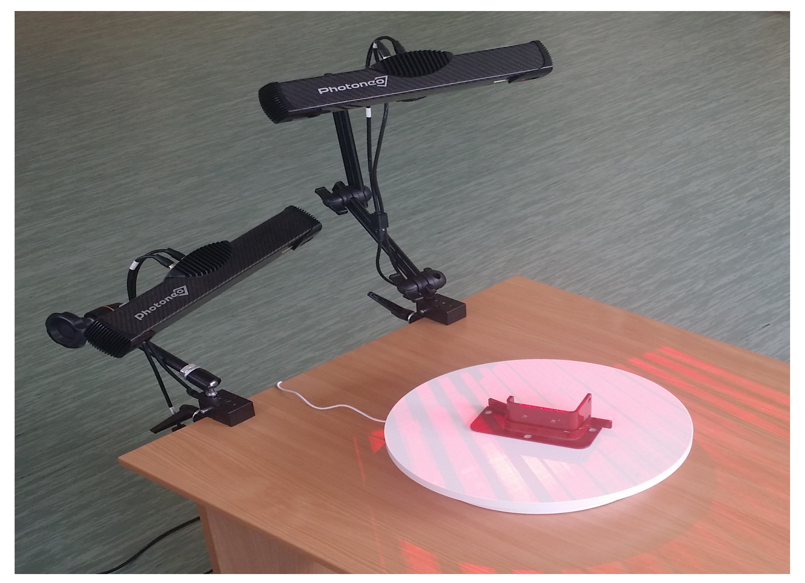
For real experiments, a 3D scanning solution from Photoneo [29] was used; see Figure 8. The system consisted of two PhoXi 3D Scanners (size M) mounted at different heights above a motorized turntable. These three devices were connected to a PC running the software PhoXi 3D Meshing that was responsible for controlling the turntable, acquiring individual scans from the scanners, and finally merging and trimming the point clouds to obtain the resulting single point cloud.

6. Experimental Results

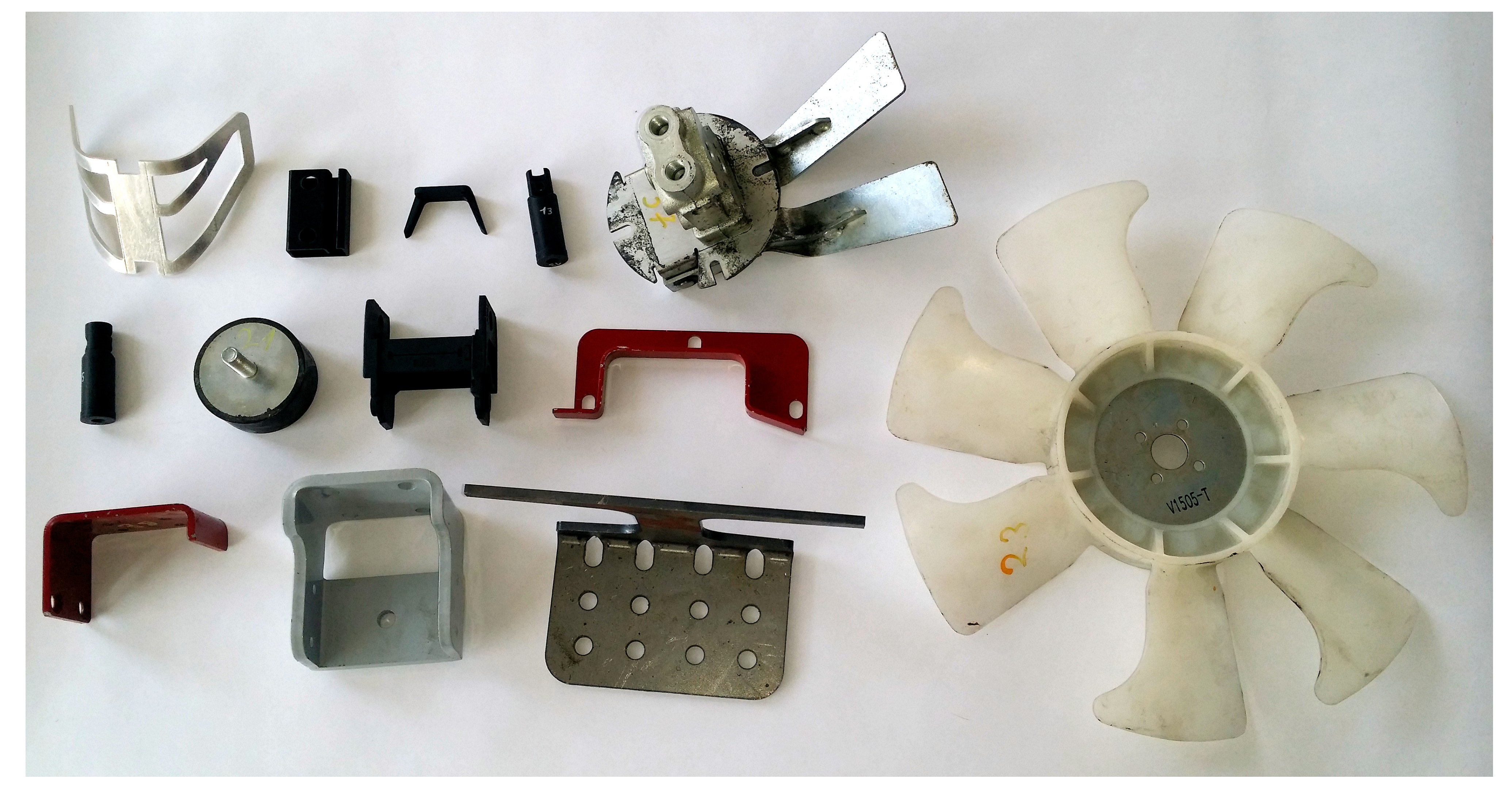
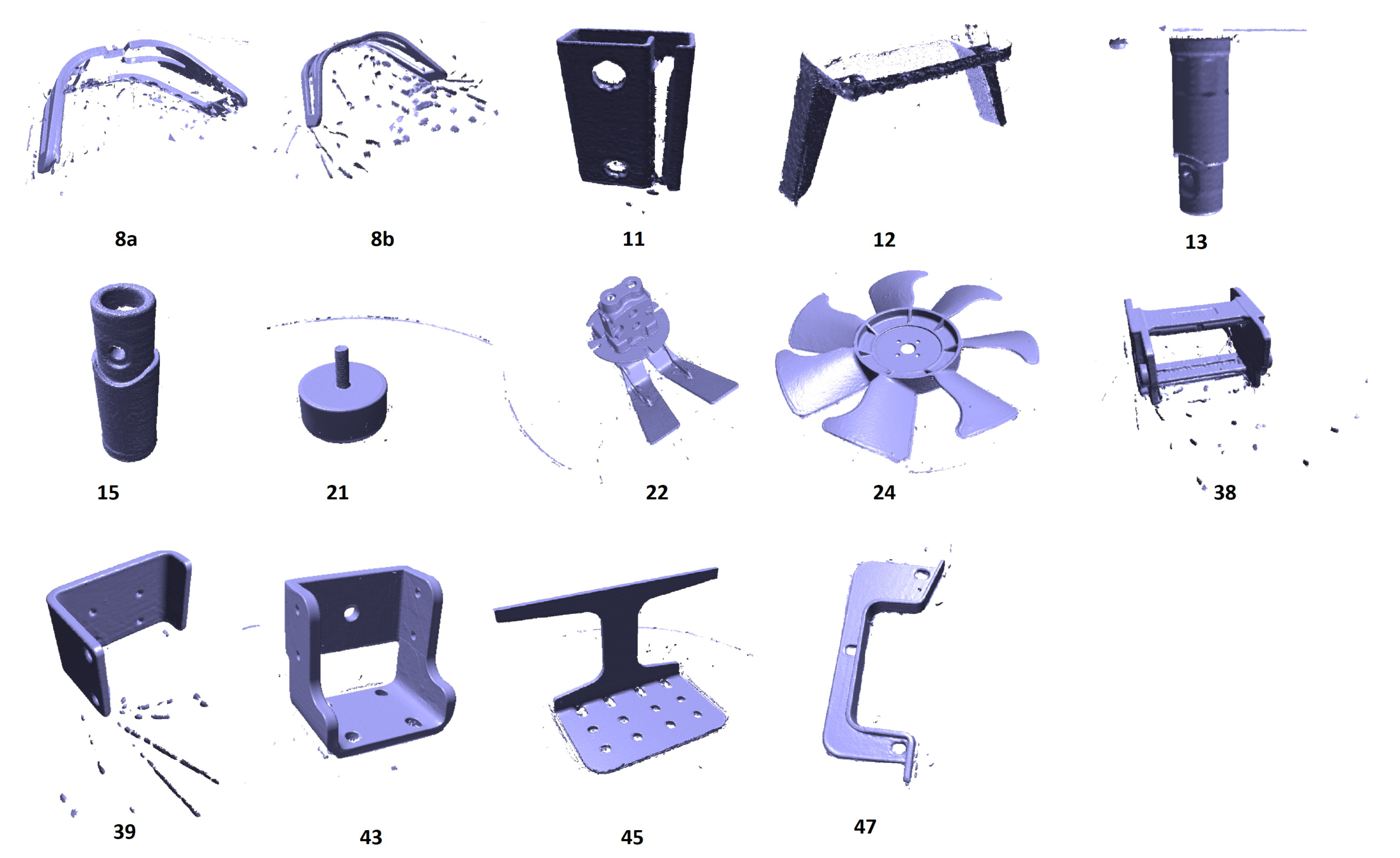
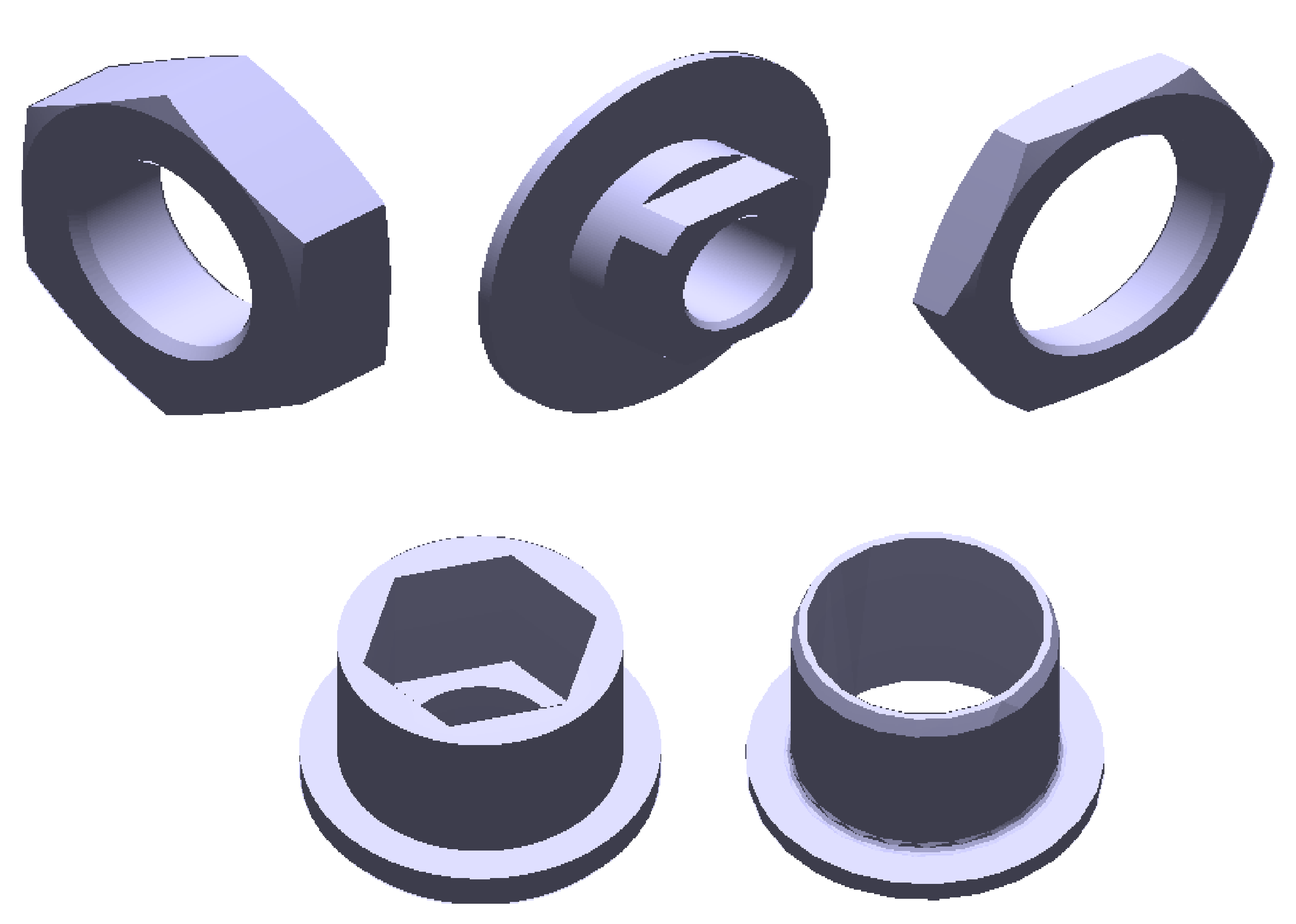
We considered a collection of 29 mechanical components, a subset of which is displayed in Figure 9. The objects were scanned in our lab; see Figure 10. The database of STL models comprises the 29 models of the scans and additional 360 models.

First, each model was preprocessed by the hierarchical PCA and the method of decomposition into geometric primitives and the resulting hierarchies; see Figure 4. The distances and angles among the primitives were stored in their respective database. This step is displayed in Figure 1 on the left. Processing of a model in MATLAB takes cca 5 min on a common laptop with a 4-quad Intel i7 processor. The overall database of 389 models was processed in 33 h, which is fine since the preprocessing step is performed once, prior to scanning.

Secondly, for each of the 29 scans, we performed a postprocessing step, as depicted in Figure 1 on the right. After an eventual noise filtering, we applied the hierarchical PCA to the point cloud of the scan and saved the resulting binary tree of triples of eigenvalues. We preselected a collection of candidate models so that the topology of the trees must match and the eigenvalue triples match in the euclidean norm at 90% and more. This preselection took a few seconds. 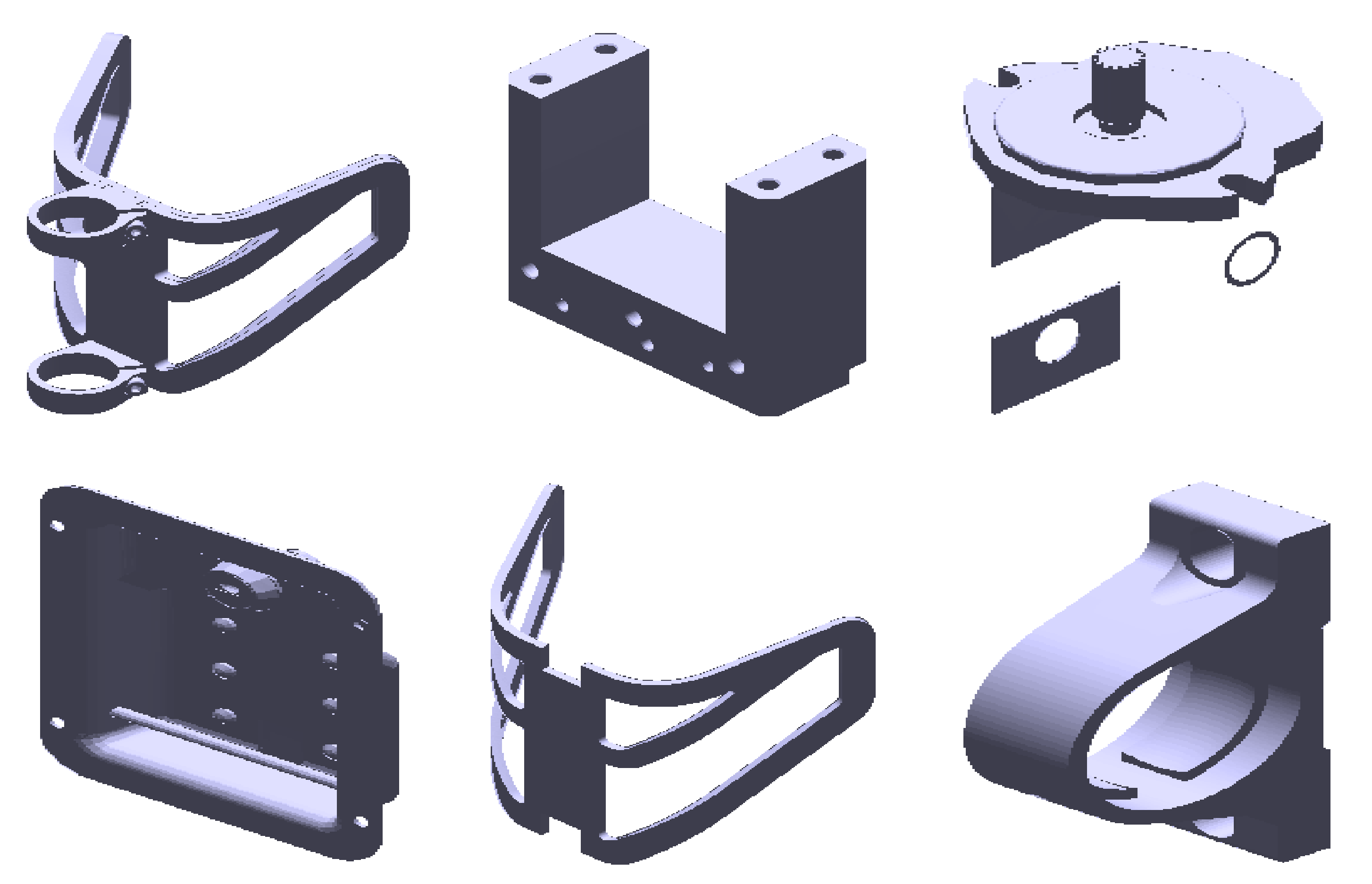A typical example of successful use of the hierarchical PCA is depicted in Figure 11, where only 6 candidates were considered after 2 levels of PCA while the right one was ranked first. On the other hand, the hierarchical PCA can hardly distinguish among the objects depicted in Figure 12. For each of the 29 scans, the method delivered a collection containing the right model, though some of the collections comprise about 50 models.

Finally, we took the list of candidates preselected by the hierarchical PCA and completed the matching procedure using the method of decomposition into geometric primitives. We counted the relative amount of planar and cylindrical primitives that have the same (under a tolerance) mutual distances and angles in both the scanned and model point clouds. The algorithm worked fast and safely for all of the 29 scans and the 389 models. The efficiency of the method of decomposition into geometric primitives is depicted in

Table 1. Matching results of the method of decomposition into geometric primitives. The first column comprises the identification numbers (IDs) of the 29 scans. Notice that object 8 was scanned twice; see also Figure 10. The next 5 columns display the IDs of the 5 best matched candidates from the collection of 389 models. The percentual score is the amount of primitives in the model that match the primitives of the scan. This amount is divided by the total amount of primitives in the scan (and multiplied by 100%).

Scan ID	Top-5 Models
	Model ID: Matching-Score
1	1: 38%	68: 25%	87: 25%	271: 25%	292: 25%
2	2: 50%	164: 36%	165: 36%	13: 29%	15: 29%
3	3: 42%	22: 33%	45: 33%	135: 33%	158: 33%
7	7: 63%	3: 21%	8: 21%	38: 21%	43: 21%
8a	8: 56%	194: 40%	91: 24%	6: 16%	7: 16%
8b	8: 66%	13: 28%	15: 28%	7: 21%	6: 14%
9	9: 38%	6: 25%	135: 25%	159: 25%	1: 13%
11	11: 88%	4: 47%	215: 47%	5: 35%	47: 35%
12	12: 87%	4: 27%	5: 27%	6: 27%	17: 27%
13	13: 83%	15: 33%	26: 33%	64: 33%	127: 33%
15	15: 50%	13: 35%	26: 30%	37: 30%	120: 30%
17	17: 53%	43: 27%	205: 27%	210: 27%	215: 27%
20	20: 88%	186: 59%	321: 41%	135: 35%	153: 35%
21	21: 80%	27: 40%	50: 40%	70: 40%	79: 40%
22	22: 83%	37: 31%	189: 31%	370: 31%	74: 29%
24	24: 85%	22: 46%	196: 46%	321: 38%	31: 31%
26	26: 84%	43: 54%	153: 54%	169: 54%	176: 54%
28	28: 86%	47: 64%	152: 64%	27: 57%	304: 57%
29	29: 50%	224: 22%	272: 22%	319: 22%	22: 17%
30	30: 38%	91: 31%	174: 31%	319: 31%	191: 23%
32	32: 88%	28: 38%	139: 31%	142: 31%	54: 25%
36	36: 71%	89: 71%	63: 57%	69: 57%	155: 57%
38	38: 92%	212: 42%	129: 33%	167: 33%	218: 33%
39	39: 75%	370: 42%	318: 38%	74: 33%	29: 29%
41	41: 62%	5: 29%	29: 29%	332: 29%	190: 24%
43	43: 93%	93: 31%	159: 31%	240: 31%	4: 28%
45	45: 73%	205: 29%	66: 24%	11: 18%	27: 18%
47	47: 78%	350: 39%	130: 35%	294: 35%	22: 30%
50	50: 71%	221: 71%	160: 57%	34: 43%	35: 43%

. As many as 27 scans were uniquely matched to their counterparts from the database, while in the remaining two cases—scans 36 and 50—there was only one additional candidate besides the correct model. The overall computation took 5 min in MATLAB using the PCL library (Image Toolbox).

7. Conclusions

In this paper, we dealt with matching 3D scans of mechanical components to an STL triangulation from a database. This problem is of interest in all domains where the identification of an a priori unknown object is required, e.g., when searching for a drawing of a damaged component. We presented an application of principal component analysis, which turned out to be very fast but lacked robustness in the case of objects differing by small details. Therefore, we developed yet another method that is based on decomposition of the point cloud into planar and cylindrical primitives. The method compares point clouds in terms of mutual properties between the primitives such as distance and angle. The second method turned out to be very robust but computationally demanding. Hence, successive application of the methods is the right choice, minimizing the computational effort while preserving the robustness.

Our work on hierarchical PCA was inspired by [4,5], where the authors used the method for clustering of 3D surface meshes into binary trees. The method is invariant with respect to rigid body modes, which may make it superior when compared, for instance, to oct-tree algorithms. The method of decomposition into geometric primitives was inspired by the group at University of Bonn [6,10,11,12]. Their work applies mostly in the area of architecture. Many similar approaches were published in geosciences when scanning terrain or in urban sciences [10,11,12,13]. In [14], the weuthors are concerned with correlations among clusters of points, which is in a sense similar to our PCA. The paper in [16] combined PCA and RANSAC to identify planar walls of buildings.

In the context of the abovementioned references, the main contribution of our work is that we applied the methodology in robotics, where most researchers have been so far concerned with artificial intelligence techniques such as deep neural networks or support vector machines. However, such approaches are computationally demanding. In our opinion, it is worth tailoring methods to the problem structure, namely, to make use of the geometrical features of point clouds and STL models. We follow exactly this purely geometrical approach. Obviously, depending on the taste of the researchers, it can be given us a priori knowledge, e.g., to the deep neural network.

In future research, we plan to accelerate the process of primitive pairing. Towards this aim, we will replace the complete graph approach, which leads to pairwise features among all the primitives, with a dense graph approach, where we will compute the pairwaise features only among the primitives that are geometricaly connected. Another improvement is with regards to robustness. We will enhance the decomposition into planar and cylindrical geometric primitives using decomposition into straight and elliptical edges that arise via intersections of the primitives. Then, we will again apply the graph approach to assemble mutual pairwise features among the edges, which will make the matching more robust.

In order to accelerate the most computationally expensive algorithm in our methodology, which is matching using the method of decomposition into geometric primitives, we shall employ parallelism so that evaluations of matching scores of point-cloud couples within the collection will be performed concurrently.

Finally, inspired by [18,19,20], it will be worth implementing yet another method, the nonlinear least-square minimization approach. In this method, we will select representative points from the scanned point cloud and we will minimize their distances from the STL models. We plan to employ Newton-based methods with global minimization strategies.

References

- Pearson, K. On lines and planes of closest fit to systems of points in spaces. Philos. Mag. 1901, 2, 559–572. [Google Scholar] [CrossRef]
- Hotelling, H. Analysis of a complex of statistical variables into principal components. J. Educ. Psychol. 1933, 24, 417–441. [Google Scholar] [CrossRef]
- Jolliffe, I.T. Principal Component Analysis, 2nd ed.; Springer: New York, NY, USA, 2002. [Google Scholar]
- Rjasanow, S.; Steinbach, O. The Fast Solution of Boundary Integral Equations; Springer: Berlin/Heidelberg, Germany, 2007. [Google Scholar]
- Lukáš, D.; Kovář, P.; Kovářová, T.; Merta, M. A parallel fast boundary element method using cyclic graph decompositions. Numer. Algorithms 2015, 70, 807–824. [Google Scholar] [CrossRef]
- Schnabel, R.; Wahl, R.; Klein, R. Efficient RANSAC for point-cloud shape detection. Comput. Graph. Forum 2007, 26, 214–226. [Google Scholar] [CrossRef]
- Zhang, J.; Cao, J.; Liu, X.; Wang, J.; Liu, J.; Shi, X. Point cloud normal estimation via low-rank subspace clustering. Comput. Graph. 2013, 37, 697–706. [Google Scholar] [CrossRef]
- Zhao, J.; Zong, C.; Cao, L.; Chen, S.; Liu, G.; Xu, J.; Xin, S. Automatically modeling piecewise planar furniture shapes from unorganized point cloud. Comput. Graph. 2020, 90, 116–125. [Google Scholar] [CrossRef]
- Tran, T.T.; Cao, V.T.; Laurendeau, D. Extraction of cylinders and estimation of their parameters from point clouds. Comput. Graph. 2015, 46, 345–357. [Google Scholar] [CrossRef]
- Schnabel, R.; Wessel, R.; Wahl, R.; Klein, R. Shape Recognition in 3D Point-Clouds. In Proceedings of the 16-th International Conference in Central Europe on Computer Graphics, Visualization and Computer Vision’2008, Plzen, Czech Rebuplic, 4–7 February 2008; pp. 65–72. [Google Scholar]
- Schnabel, R.; Degener, P.; Klein, R. Completion and reconstruction with primitive shapes. Comput. Graph. Forum 2009, 28, 503–512. [Google Scholar] [CrossRef]
- Ochmann, S.; Vock, R.; Wessel, R.; Klein, R. Automatic reconstruction of parametric building models from indoor point clouds. Comput. Graph. 2016, 54, 94–103. [Google Scholar] [CrossRef]
- Vock, R.; Dieckmann, A.; Ochmann, S.; Klein, R. Fast template matching and pose estimation in 3D point clouds. Comput. Graph. 2019, 79, 34–45. [Google Scholar] [CrossRef]
- Zhang, Z.; Zhang, L.; Tong, X.; Zhen, W.; Guo, B.; Huang, X.; Yuebin, W. A multilevel point-cloud-based discriminative feature for ALS point cloud classification. IEEE Trans. Geosci. Remote Sens. 2016, 54, 3309–3321. [Google Scholar] [CrossRef]
- Yu, Y.; Li, J.; Guan, H.; Jia, F.; Wang, C. Three-dimensional object matching in mobile laser scanning point clouds. IEEE Geosci. Remote Sens. Lett. 2014, 12, 492–496. [Google Scholar]
- Yang, B.; Wei, Z.; Li, Q.; Li, J. Semiautomated building facade footprint extraction from mobile LiDAR point clouds. IEEE Geosci. Remote Sens. Lett. 2013, 10, 766–770. [Google Scholar] [CrossRef]
- Rente, P.; Brites, C.; Ascenso, J.; Pereira, F. Graph-based static 3d point clouds geometry coding. IEEE Trans. Multimed. 2018, 21, 284–299. [Google Scholar] [CrossRef]
- Somani, N.; Cai, C.; Perzylo, A.; Rickert, M.; Knoll, A. Object recognition using constraints from primitive shape matching. In Proceedings of the International Symposium on Visual Computing, Rethymnon, Crete, Greece, 29–31 July 2013; pp. 783–792. [Google Scholar]
- Besl, P.; McKay, H.D. A method for registration of 3-d shapes. IEEE Trans. Pattern Anal. Mach. Intell. 1992, 14, 239–256. [Google Scholar] [CrossRef]
- Roth, G.; Levine, M.D. Extracting geometric primitives. Image Underst. 1993, 58, 1–22. [Google Scholar] [CrossRef]
- Jiang, H.; Drew, M.; Li, Z.N. Matching by linear programming and successive convexification. IEEE Trans. Pattern Anal. Mach. Intell. 2007, 29, 959–975. [Google Scholar] [CrossRef] [PubMed]
- Rusu, R.B. Semantic 3D Object Maps for Everyday Robot Manipulation; Springer: Berlin/Heidelberg, Germany, 2013. [Google Scholar]
- Mahmoudi, M.; Sapiro, G. Three-dimensional point cloud recognition via distributions of gemetric distances. Graph. Model. 2009, 71, 22–31. [Google Scholar] [CrossRef]
- Zia, Z.; Stark, M.; Schiele, B.; Schindler, K. Detailed 3d representations for object recognition and modeling. IEEE Trans. Softw. Eng. 2013, 35, 2608–2623. [Google Scholar] [CrossRef] [PubMed]
- Hilaga, M.; Shinagawa, Y.; Komura, T.; Kunii, T.L. Topology matching for fully automatic similarity estimation of 3d shapes. In Proceedings of the 28th Annual Conference on Computer Graphics and Interactive Techniques, Los Angeles, CA, USA, 12–17 August 2001; pp. 203–212. [Google Scholar]
- Gonzalez, J.P.; Luna-Madrigal, F.; Pina-Ramirez, O. Deep learning point cloud registration based on distance features. IEEE Lat. Am. Trans. 2019, 17, 2053–2060. [Google Scholar] [CrossRef]
- Rusu, R.B.; Cousins, S. 3D is here: Point Cloud Library (PCL). In Proceedings of the IEEE International Conference on Robotics and Automation (ICRA), Shangai, China, 9–13 May 2011; pp. 65–72. [Google Scholar]
- The Point Cloud Library. Available online: http://pointclouds.org (accessed on 19 March 2020).
- Photoneo, PhoXi 3D Meshing. Available online: https://www.photoneo.com/3d-model-creation/ (accessed on 12 February 2020).