Combining Chemical Composition Data and Numerical Modelling for the Assessment of Air Quality in a Mediterranean Port City

Abstract

The aim of this study is to characterize the air quality in a Mediterranean port city. The impact of ship emissions on both gaseous and particulate pollutants has been investigated through an integrated methodology which includes atmospheric flow and dispersion numerical modelling as well as chemical composition and statistical analyses. Specifically, chemical compositional data (ionic fraction, carbonaceous compounds, and metals) of PM_2.5 were acquired during an experimental field campaign carried out in the port city of Brindisi (Apulia Region, Southern Italy). The sampling site was located on the roof of a building (ASI) within the port area. Given the complexity of the site in which both domestic buildings and a large industrial area are present, analyses were done by selecting different wind sectors to test different techniques to discriminate between sources. Linear Discriminant Analysis (LDA) and Principal Component Analysis (PCA) were applied to evaluate statistical differences in the composition of PM_2.5 sampled within the area when the sampling site was downwind to the port or to the urban-industrial area. Only LDA allowed to discriminate the separation between urban-industrial and port macroareas. Those results were further confirmed in terms of PM_2.5 concentrations directly associated to ship emissions using a coupled modelling approach. The mesoscale model BOLCHEM was used to investigate the contribution of ship emissions both on primary and secondary PM_2.5 concentration in the area surrounding the port, as well as on PM₁₀, NO_X and O₃ concentrations. Then, the model was coupled offline with the local dispersion model ADMS-Urban. The adopted approach was crucial to evaluate the spatial distribution of the impact of ship emissions. BOLCHEM results showed that in the cell of the port the average impact of ship emissions on NO_X was 37.6%, and −11.7% on O₃. The average impact on PM_2.5 was 6.1%, distributed between primary (2.7%) and secondary fraction (3.4%). At local scale, the analysis of high-resolution modelling results obtained from ADMS-Urban highlighted that, at ASI position, the impact of ship emissions on PM_2.5 was 6.8% when the sampling site was positioned downwind to the port area and reduced to lower than 3.0% at about 2 km from the sources.

1. Introduction

Air pollution is among the most critical environment issue and it is strictly linked to climate change through emissions, processes, chemistry, and dynamic of the atmosphere [1,2]. Atmospheric particles, for example, play crucial roles in deteriorating air quality and affecting human health, in the pollution transfer to ecosystems, in the direct and indirect effects on atmospheric radiative balance, and in the climate system [3,4,5]. The identification and quantification of air pollution sources are then important tasks for abatement strategies and mitigation actions. Ship emissions represent a large and growing contribution to the total emissions from the transportation sector. In contrast to the progress in reducing anthropogenic emissions on land since the 1990s due to regulation in Europe, emissions from marine transportation have continued to increase [6]. Nowadays, their effects on atmospheric pollution and climate are not negligible. Key emitted compounds are carbon dioxide (CO₂), nitrogen oxides (NO_X), carbon monoxide (CO), volatile organic compounds (VOC), sulphur dioxide (SO₂), black carbon (BC), and organic aerosol (OA) [7]. Nearly 70% of ship emissions occur within 400 km of coastlines and they contributed to increase the air pollutants concentration level in coastal areas and harbour cities [8,9]. The effect on PM_2.5 concentration and sulphur and nitrogen deposition in European coastal regions are greater when emissions occur near the coast rather than offshore, while for ozone (O₃) larger contributions are from open sea shipping [10,11]. Several authors have estimated the impact of ship emissions in the Mediterranean area, where, especially during summer months, meteorological and chemical conditions favour the formation of secondary gases and aerosols. Marmer and Langmar [12] employed a regional atmospheric-chemistry model to determine the origin, the seasonal variability of secondary gases and aerosol and their effects on climate. Tagaris et al. [13] found that shipping emissions played an important role on O₃ levels compared to road transport sector near the coastal zone. The effect of international shipping on air pollution have been studied in several papers [14,15]. Eyring et al. [14] quantified the global impact of shipping on atmospheric chemistry and radiative forcing, as well as the associated uncertainties. Different ship emission scenarios, including ship emissions increase up to 2030, were investigated. It was found that under pessimistic anthropogenic sources emissions scenario, increasing emissions from shipping would significantly counteract the benefits derived from reducing SO₂ emissions from all other anthropogenic sources. Sofiev et al. [15] evaluated the impact of low-sulphur marine fuels in global shipping on public health and on climate, the last in terms of net aerosol forcing, for the year 2020. Considering that the International Maritime Organization (IMO) proposed the change in the standards of sulphur in fuel oil from 3.5% (by mass) to 0.5% after 1 January 2020, they found that lower sulphur fuels reduced ship-related premature mortality and morbidity by 34% and 54%, respectively, and radiative cooling from ship aerosols by about 80%, equating to a 3% increase in current estimates of total anthropogenic forcing.

Urban area with ports, often in combination with petrochemical and energy intensive industries, are thus particularly exposed to ship emissions. Several studies have demonstrated advancements in the assessment of shipping emission impact on air quality and human health and in the implementation of control techniques, technology improvements in ship engines, and mitigation measures in port areas [16,17]. Recently, Sorte et al. [18] reviewed the status of the air quality measured in harbour areas and found that emissions from the maritime transport sector should be considered as a significant source of NO₂, PM₁₀, and PM_2.5. Depending on the measurement period and on the geographical area, in Europe the average ambient NO₂ and PM₁₀ concentrations associated with shipping emissions ranges in 12–107 μg/m³ and 2–50 μg/m³, respectively. In urban areas close to population clusters, such as Taranto and Naples, ship emissions led to several exceedances of the NO₂ annual limit. The SO₂ concentrations measured in different case studies have instead relatively low value, as a consequence of the mitigation strategies which regulated the SO₂ ship emissions in EU harbours from January 2010 (MARPOL Annex VI and the Directives 2005/33/EU and 2012/33/EU). For example, Schembari et al. [19] performed SO₂ concentration measurements from August to October 2009 and 2010 at an automated monitoring station placed on a cruise ship following a fixed weekly route in the Western Mediterranean. They found an average daily mean concentration decrease of about 66% in all the analysed EU harbours after the implementation of the aforementioned Directive. Buccolieri et al. [20], using numerical simulations, found for the port of Brindisi (South-East Italy), a significant SO₂ concentration reduction up to 60% in the summer period of the year 2012.

Brindisi port city is one of those included in the CESAPO project (Contribution of Emission Sources on the Air quality of the Port cities in Greece and Italy) of the European Territorial Cooperation Programme Greece–Italy 2007–2013 and in the POSEIDON project (Pollution monitoring of ship emissions: an integrated approach for harbours of the Adriatic basin) of the MED program 2007–2013. Relevant findings from field experimental champaigns carried out in the frame of the CESAPO project have been documented in Cesari et al. [21] and Donateo et al. [22]. These studies highlighted the difficulty of identifying the impact of ship sources in complex urban-industrial-port scenarios and open up to the application of integrated methodologies in which numerical modelling is beneficial to the interpretation of chemical analyses.

Focusing on chemical characterization only, there exist methods based on the evaluation of monitoring data. This has the advantage of being simple with a low impact of mathematical manipulation in the data treatment. In addition, statistical methods can be used as complementary to other approaches to guarantee robustness to findings. One of the main differences between several approaches is the degrees of knowledge required about the pollution sources. Chemical mass balance (CMB) can be performed when the changes of the source profiles between the emitter and the receptor may be considered minimal and secondary aerosols must be included not as components of emission sources profile but as single chemical compounds. Multivariate methods (e.g., Absolute Principal Component Analysis, Positive Matrix Factorization, Factor Analysis) may contemplate a mixture of emission sources, as opposed to clearly independent source profiles [23,24].

A different approach is based on Chemical and Transport Models (CTMs). These models include the description of the main physical and chemical processes involved in pollutant transport and transformation and allow the prediction of air quality at various spatial and temporal scales, as well as of future scenarios. Modelled concentrations are influenced by model formulation [25,26] and by the input emissions. Marmer et al. [27] assessed the accuracy of three different commonly used ship emission inventories, confirming that the air pollution levels in the Mediterranean area are significant, but strongly dependent on the applied inventory. Source apportionment tools can be implemented in numerical models [28] and they can be used in combination with receptor models [29].

Scope and Content of the Paper

In this context, the aim of this paper is to characterize air quality and ship emissions impact on both gaseous and particulate matter in the city of Brindisi using an integrated approach that includes the most up-to-date techniques available in the realm of those current in use and often applied in isolation and rarely in combination. While the first part of the work is based on chemical and statistical analyses of PM_2.5, the second part is based on atmospheric dispersion numerical modelling. The modelling approach has been first employed to evaluate the concentration levels of NO_X, O₃, PM_2.5, and PM₁₀ in the port area and then integrated with measurements to evaluate the impact of ship emissions on pollutants concentration in the study area, with a focus on PM_2.5.

2. Site Description and Techniques for Data Analyses

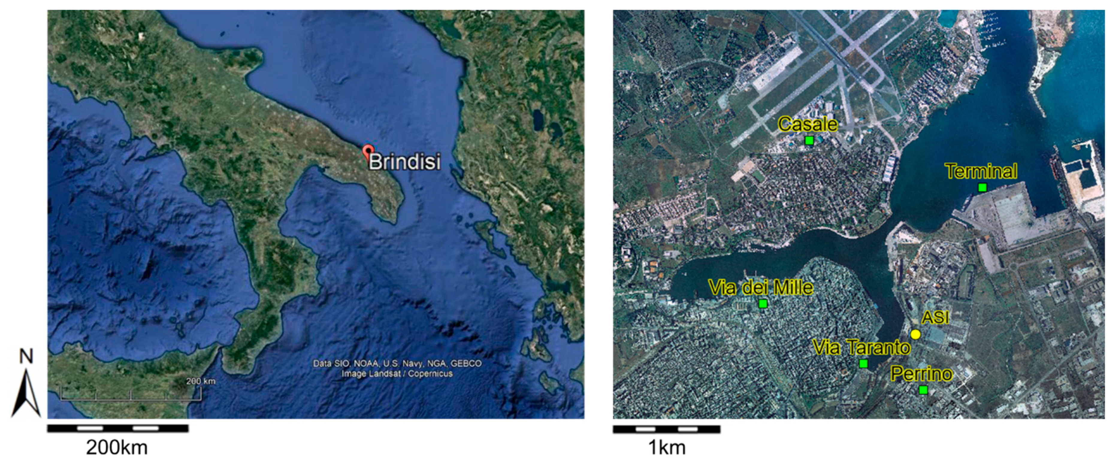
2.1. Experimental Site and General Methodology

The experimental site was set in the Brindisi port-industrial area (Figure 1). The experimental campaign was part of the CESAPO project as largely described in Cesari et al. [21]. Here, we report only those aspects relevant to the scope of this paper. Brindisi is a city with about 86,000 inhabitants located in the Apulia Region, Southern Italy. The area is characterized by a complex scheme of emission sources which need to be identified with respect to the PM_2.5 sampling site located on the roof of the ASI (Consorzio per l’Area di Sviluppo Industriale) building at 13 m above the ground level. Broadly speaking, emissions can be categorized as urban emissions, port-related emissions with port traffic accounted for more than 9.5 million tons, 520,000 passengers, and 175,000 vehicles and industrial emissions. With respect to the sampling site, the port is located at NNE to WNW, airport emissions are located at NW, while petrochemical emissions, power-plant emissions, and several artisan activities are located at SSW.

To estimate the impact of the port area on the city, an evaluation of the existence of a statistical difference among PM_2.5 samples collected in the port area according to the prevailing winds has been performed using a linear discriminant analysis. Given the specific layout of the port of Brindisi (Figure 1), and in accordance with Cesari et al. [21], for winds in the sector NNE to WNW (22.5°–292.5°) the sampling site was directly affected by the urban and industrial areas, while for winds in the sector WNW to NNE (292.5°–22.5°), the sampling site was affected directly by the port area. In the first case (referred to as Urban-Industrial) a total of 38 days were considered in the analysis (8 days in June, 8 days on July, 5 days in August, 10 days in September, and 7 days in October); in the second case (referred to as Port) 55 days were considered (15 days in June, 11 days in July, 10 days in August, 8 days in September, and 11 days in October). Please note that PM_2.5 samples were collected for 24 h, starting from 00:00 to 24:00. Each sample was representative of the sampling day and the prevailing wind direction was obtained from meteorological data measured close to the study site by calculating the median of measured wind directions.

It is known that organic matter and elemental carbon account for a relevant part of PM_2.5, ranging between 20 and 45% [30]. With this in mind, the chemical characterization of pollution sources on the PM_2.5 samples collected in the port of Brindisi, previously reported in Cesari et al. [21], has been extended to organic carbon and elemental carbon and in this respect this work completes the analyses previously reported. Principal Component Analysis has been applied to a larger and more comprehensive data set with respect to Cesari et al. [21] with the aim of deriving more realistic source profiles through factor loadings of the variables affecting the receptor site. Further, chemical mass closure has been used for sources quantification.

Chemical characterization of PM_2.5 has been then completed with numerical investigations by combining the mesoscale model BOLCHEM [31,32] and the local scale advanced-Gaussian dispersion model ADMS-Urban [33]. BOLCHEM simulations were performed for the whole measurement campaign period (June-October 2012) to reproduce hourly pollutants concentration, both for gaseous and particulate and to calculate mean concentration over the area, at regional scale. Simulation results were compared with measurements at the sampling site (ASI) and at monitoring stations managed by ARPA-Puglia (Environmental Protection Agency of Apulia Region, https://www.arpa.puglia.it/pagina2795_aria.html (accessed on 1 March 2021)) (Figure 1). The impact of ship-related emissions of PM_2.5 on PM_2.5 and PM₁₀ concentration, as well as of NO_X emissions on O₃ concentration, has been also estimated. The spatial distribution of concentration levels at local scale has then been assessed using ADMS-Urban in which background concentrations were calculated by the mesoscale model.

2.2. Gravimetric and Chemical Analysis

Detailed description of chemical analysis methods could be found in Cesari et al. [21]. PM_2.5 daily samples were collected by using two sequential low-volume samplers (2.3 m³h⁻¹, EN12341), using two different substrates: Teflon collected by a Thermo ESM Andersen (FH95SEQ) sampler and quartz fibre by an Explorer Plus (Zambelli) sampler. Each sampling starts at midnight. In total 100 Teflon substrate samples and 100 quartz substrate samples were collected from June to October 2012. Wind, atmospheric pressure, relative humidity, and temperature were measured from the meteorological station located close to the study site.

After stabilizing for 48 h in controlled environment (constant humidity and temperature), all filters were weighted with an analytical balance (Sartorius CP2/F, reading precision 1 μg) before and after sampling. The daily concentrations of quartz and Teflon substrates were similar (Pearson correlation coefficient of 0.87 and an average value of 15.1 µg m⁻³ and of 14.2 µg m⁻³ for Teflon and quartz substrates, respectively). Teflon substrates measurements showed lower uncertainty than those on quartz substrates, then they were taken as reference for PM_2.5.

Teflon samples were used to measure water-soluble species (Na⁺, K⁺, Mg²⁺ and Ca²⁺, SO₄²⁻, NO₃⁻, NH₄⁺, Cl⁻), water-soluble inorganic carbon (WSIC) and water-soluble organic carbon (WSOC). Two aliquots of 5 mL of deionized water were used to extract the soluble ionic species by ultrasonic agitation for 20 min. Chemical analysis was performed using a Dionex DX500 (Dionex, Sunnyvale, CA, USA) Ion Chromatography system, and the method is reported in Cesari et al. [21].

WSOC and WSIC were measured using a Shimadzu TOC analyser (model 5050, Shimadzu corporation) with high-temperature (680 °C) Pt-catalysed oxidation coupled to non-dispersive infrared (NDIR) gas detection of CO₂ [21].

Quartz samples were used for the determination of 16 metal concentrations and OC and EC measurements. 8 elements (Ni, Cu, V, Mn, As, Pb, Cr, Sb) were analysed by Graphite Furnace Atomic Absorption Spectroscopy (GF-AAS, Perkin Elmer Analyst 600 System) and 8 elements (Ca, Mg, Na, K, Fe, Al, Zn, and Ti) by Inductively Coupled Plasma Atomic Emission Spectroscopy (ICP-AES, Varian Liberty 110 spectrometer). 1 mL of H₂O₂, 2 mL of HF and 4 mL of HNO₃ were used for acid digestion in a MILESTONE MLS 1200 MEGA (FKV) microwave oven. 0.7 g of H₃BO₃ was added after cooling to complex fluoride ions and to dissolve fluoride salts [21].

Organic/Elemental carbon (OC and EC) were analysed by a carbon aerosol analyser (Sunset Laboratory Inc., Tigard, OR, USA) [34] using NIOSH protocol [35]. The carbonaceous fraction of PM_2.5 was detected on a 1.5 cm² quartz substrate punch. Uncertainties in EC and OC measurements were of about 5% ± 0.2 μg cm⁻². For sampling of quartz substrate a denuder was not used [36,37].

2.3. Statistical Treatment of Data: Principal Component Analysis and Linear Discriminant Analysis

Multivariate statistical techniques were used to grossly discriminate between the main sources acting on the port city by ensuring that the tested dataset had a suitable number of objects. The analyses were carried out using the R statistical software (www.r-project.org (accessed on 1 March 2021)) and an auto-scaling procedure.

Principal Component Analysis (PCA) was applied to a dataset of daily PM_2.5 samples (objects). The PCA performs orthogonal linear combinations of the auto-scaled variables, generally by using the correlation matrix. Linear combinations are called principal components scores, while their coefficients are referred to as principal component loadings. The Principal Components are obtained according to the maximum variance criterion, i.e., each successive component is an orthogonal combination of the original variables, so that it covers the maximum of the variance not accounted for by the previous components. The strength of the PCA is that it is based on the data collection evolving in a specific site (receptor). Moreover, it does not require an a priori knowledge about the sources [38,39,40]. Therefore, this is the most suitable technique to discriminate between different sources acting on a site according to meteorological/climatological conditions.

The Linear Discriminant Analysis (LDA) was applied to a dataset of daily PM_2.5 samples (cases), considering the two prevailing wind direction observed as categories (or groups) and 20 chemical components of PM_2.5 as variables. LDA identifies which variables allow to discriminate between two or more groups, determining how these groups can differ as concern the mean of a variable and then using this one to classify new cases. As happens in PCA, in LDA the first discriminates function considered supplies the most discrimination between groups, the second supplies second most, and so on [39,41,42]. In our work we performed the LDA in order to evaluate groups separation. The LDA results are generally shown by confusion matrix which contains how many errors, and which types arise in resubstitution. When there are K groups, the confusion matrix R is a K-by-K matrix with R(i,j) = the number of observations of group i that the classifier predicts to be of class j.

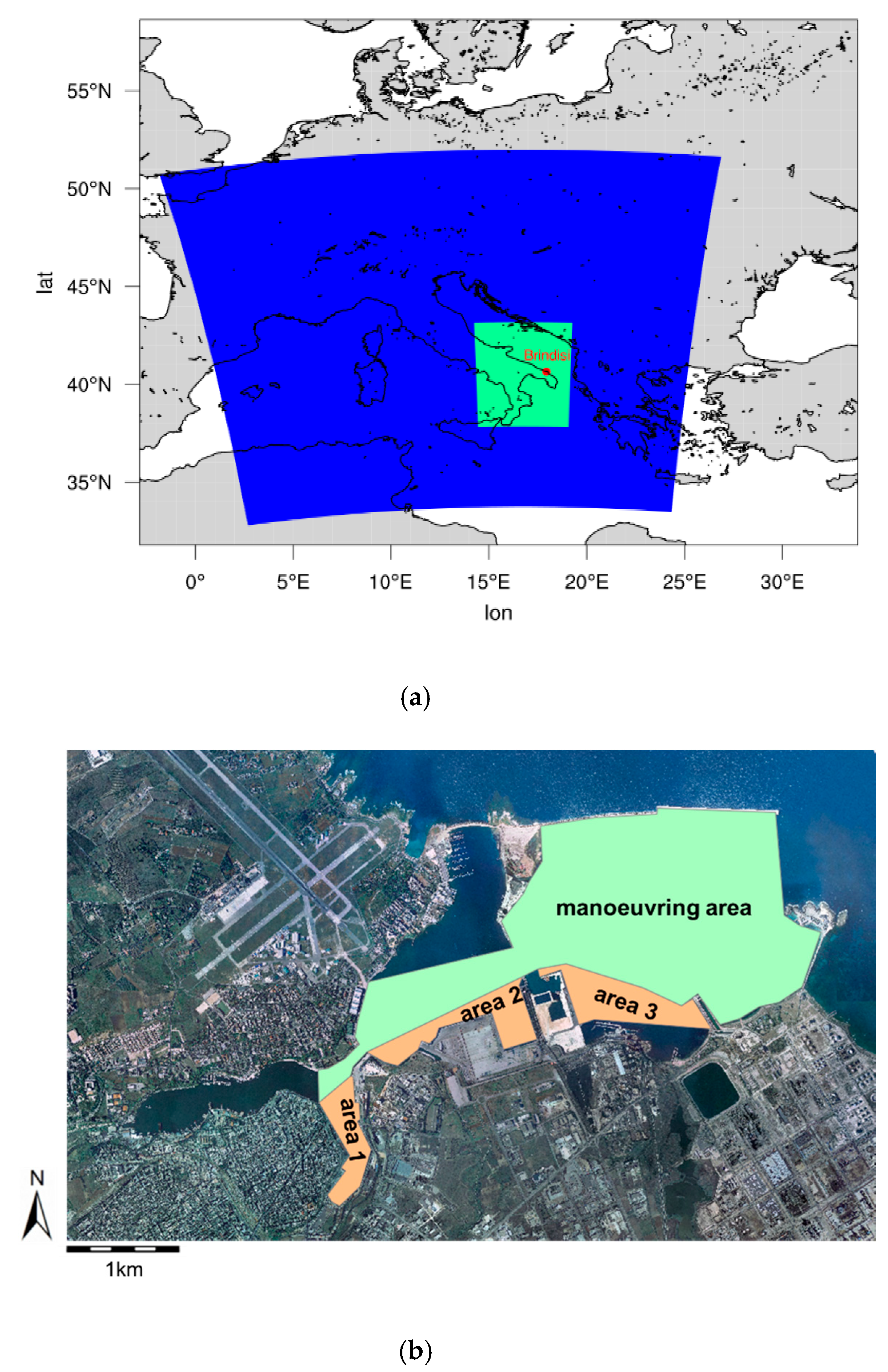
2.4. Numerical Modelling

To quantify the impact of ship emissions, two different models have been employed: BOLCHEM [31,32] and ADMS-Urban [33]. BOLCHEM simulations domain covered the Apulia region, allowing to evaluate the spatial distribution of the ship emissions impact in the area surrounding the port. ADMS-Urban, using background concentration simulated by BOLCHEM and modelling explicitly the ship emissions, allowed to evaluate the detailed spatial distribution of pollutants at a local level. Unlike BOLCHEM, ADMS-Urban uses a simplified chemical module for NO_x-VOC-O₃ chemistry and the formation of secondary aerosols is not included in the model.

2.4.1. Ship Emissions

Ship emissions were calculated (in the frame of CESAPO project, and then updated in the MED POSEIDON project) following the methodology Tier 3 of the European methodology EMEP/EEA emission inventory guidebook [43], that takes into account gross tonnage and ship typology to calculate the specific fuel consumption. The emission inventory was built considering ship by ship, i.e., every ship was represented as a single point source characterized by its own emissions rates. Emission factors for CO, NO_X, NMVOC, and PM were estimated as a function of the combination of engine type and fuel type. The considered engine types were: gas and steam turbines, diesel engines at low, medium, and high speed; for the fuel we considered: Bunker Fuel, Oil, BFO, Marine Diesel Oil, MDO, and Marine Gas Oil, MGO. We have used the statistical distribution of fuel and engine type of the ship derived from tables of world fleet data from Lloyd’s [43], since more detailed information was not available in the database supplied by the Port Informer. Emissions factor (EF) for SO₂ were calculated as a function of the percentage of content sulphur by mass (S) in the fuel, that is EF = 20*S. As for the percentage of content sulphur by mass in the fuel, we distinguished between manoeuvring and hotelling phase. For the manoeuvring phase, we considered a limit of sulphur in fuel equal to 1.5% for all passenger ships (including cruise ships), and a limit equal to 3.5% for all other ship typologies, according to the current legislation in force, the revised MARPOL Annex VI. For the hotelling phase, a limit equal to 0.1% was considered for all ship typologies. The fuel consumption was estimated according to Buccolieri et al. [20]. Ship data regarding ship movements (manoeuvring and hotelling phases) were available from the Brindisi Port Informer (http://www.porto.br.it/bpi/index.php (accessed on 1 March 2021)). Emissions rates were then calculated by considering time spent by each ship in the different phases. The uncertainties related to emission factors of the different pollutants range between 20% and 50% [43]. Furthermore, inaccurate information about fuel consumption, engine typologies, and used fuel could increase the uncertainties of the estimated emissions fluxes.

2.4.2. Models Description and Set-Up

BOLCHEM is an on-line atmospheric composition model, which comprises the hydrostatic meteorological model BOLAM [44], an algorithm for airborne transport and diffusion of pollutants, the photochemical mechanisms SAPRC90 [45] extended to describe the formation of condensable organic products and the oxidation in aqueous [46] and the aerosol dynamic model AERO3 [47]. The aerosol model is coupled with the inorganic thermodynamic equilibrium model ISORROPIA [48] and with the partitioning model SORGAM [49] for secondary organic aerosol. A full description of the model and its performance over European and Italian domain can be found in Cesari et al. [32], and a model application of estimation and inclusion of emissions from specific source is shown in Cesari et al. [50]. In the present study, the model has been used in a one-way nested grid configuration [51], with a parent domain covering Italy with horizontal resolution of 0.25° × 0.25° and a nested domain covering Apulia region at 0.06° × 0.06° horizontal resolution. Both parent and nested simulations used 50 vertical levels for the meteorology and 25 for the chemistry. We recall that the vertical coordinate is based on a hybrid, pressure-based coordinate system, in which the pure terrain-following coordinate at the model surface, gradually tends to a pure pressure coordinate with increasing height above the ground. In the adopted set up, the first vertical level height was about 20 m. The parent run was driven by initial and boundary conditions for meteorology provided by ECMWF. The simulations were re-initialised every 24 h with the ECMWF fields and lateral boundary conditions were updated every 6 h. Climatological boundary conditions provided by INERIS in the frame of the CityZen project were used for chemistry [52]. The anthropogenic emission data were based on TNO inventory for the 2010 year [53]. For the nested run, the initial and boundary conditions, both meteorological and chemical, were provided by the output of the parent simulation. The anthropogenic emissions field, developed within the CESAPO project, was based on the 2007 regional emission inventory INEMAR (INventarioEMissioni in Aria), the emission inventory ISPRA 2005 (focused on 2007 and with the addition of PM by road re-suspension and agriculture) and the emission inventory EMEP 2007. Only ship emissions from the port of Brindisi refer to the year 2010 and were calculated following the methodology described in Section 2.4.1 in order to take into account the European Directive concerning the sulphur content of maritime fuels. In both simulations, biogenic emissions, calculated run time by the model, were based on an inventory providing potential emissions and generated by NKUA (National and Kapodistrian University of Athens) in the frame of the GEMS project [54].

Two runs were performed with BOLCHEM over the inner domain: the base simulation including anthropogenic emissions from all sources, the other one switching off the ship emissions from the Brindisi port. Following the zero-out method, the difference between the concentration fields produced by the two runs then represented the contribution of ship emissions. Figure 2a shows the simulation domain.

ADMS-Urban simulations were then performed over a grid of 100 × 100 cells covering an area of 13 km × 7 km. ADMS-Urban is a multiple-source advanced Gaussian dispersion model which can simulate urban air pollution arising from industrial, domestic, and road traffic sources in urban areas using point, line, area, volume, and grid-source types. Concentration distributions are Gaussian in stable and neutral conditions, but the vertical distribution is non-Gaussian in convective conditions to take account of the skewed structure of the vertical component of the turbulence. A meteorological pre-processor calculates the required boundary layer parameters from a variety of input data (in our case data were provided by a meteorological station). One of the main advantages of the ADMS-Urban model over other dispersion models is that the boundary layer structure is based on two parameters: the Monin-Obukhov length and boundary layer height, instead of a single Pasquill-Gifford parameter. Model is time independent so there are no time steps; there are no limits to horizontal and vertical spatial resolution. No numerical methods are required except Runge Kutta for plume rise model and adaptive time stepping for chemistry. As for the chemistry, ADMS-Urban models NO_X chemistry using the 8 reaction Generic Reaction Set [55]. This scheme is a semi-empirical photochemical model which reduces the complicated series of chemical reactions involving NO_X, NO₂, and O₃ and many hydrocarbons to 8 reactions. It is employed in the following manner. Firstly, dispersion of NO_X, NO₂, and O₃ and VOC pollutants is calculated. Hourly background concentrations (in this case obtained from BOLCHEM) are then added onto these calculated concentrations. Finally, an adaptive time stepping technique is used to model the chemical reactions. Further details can be found at https://www.cerc.co.uk/environmental-software/assets/data/doc_techspec/P18_03.pdf (accessed on 1 March 2021). PM is only dispersed, and the final concentrations obtained from ADMS-Urban does not include secondary aerosols as consequence of ship emissions. The model is continually validated against available measured data obtained from real world situations, field campaigns and wind tunnel experiments. It has been validated using many experimental datasets that test different aspects of the models, for instance: ground/high level sources, passive and buoyant releases, buildings, complex terrain, chemistry, deposition, and plume visibility. These studies are both short-term as well as annual, and involve tracer gases or specific pollutants of interest (a review of studies is available at: http://cerc.co.uk/environmental-software/model-validation.html (accessed on 1 March 2021)). In this study, the input data used to run ADMS-Urban were sources parameters, source emissions, hourly meteorological data obtained from the 10 m high meteorological station located close to the study site, the surface roughness z₀ for both the study area (equal to 0.75 m being this an urban area) and for the meteorological site (equal to 0.5 m being a suburban area), and the latitude (40.38°). Only ship-related emissions were explicitly reproduced for the same period of the measurement campaign. The port was split into three hotelling areas and one manoeuvring area. Each ship was assigned and randomly positioned in the area containing its own quay and to the manoeuvring area (Figure 2b). Since data concerning geometric and emissive characteristics of sources (stack height and diameter, exit velocity, exit temperature) were not publicly available, they are estimated based on the literature (http://www.slc.ca.gov; http://www.epa.gov; http://www.arb.ca.gov (accessed on 1 March 2021)). Emission rates were calculated as described in Section 2.4.1. Typical molar NO₂ to NO_X emission ratio are between 10% and 40%; here a value of 10% has been used [56]. Overall, emissions in the hotelling phase were higher than those in the manoeuvring phase and contributed more than 95% to the total emission rates. Tests with ship emissions of the year 2010, as used in BOLCHEM, have shown no significant difference on the final calculated concentrations. The background field data were provided by BOLCHEM simulations, in the configuration with ship emissions from port of Brindisi switched off.

3. Results and Discussion

3.1. Overview on PM_2.5 Composition in the Investigated Area

A total of 100 PM_2.5 daily samples were collected to determine the concentrations of ten inorganic species, three carbonaceous components and sixteen metals. Results show that, on average, OC and EC accounted for 15.4% and 3.4% of PM_2.5 mass, respectively, while in terms of organic matter (OM) (that is obtained multiplying OC average concentration for f_OM/OC = 1.95) we obtained the 30.3% of PM_2.5 mass. Moreover OC, WSOC, SO₄², and NH₄⁺ concentrations were generally larger than 1 µg m⁻³; this result was explained by considering the expected contribution from anthropogenic sources for PM_2.5. Marine aerosol and suspended dust, that are sources mainly present in the PM coarse fraction, affected in minor amount the fine fraction.

The predominant anthropogenic species (OC, EC, WSOC, SO₄²⁻, NO₃⁻, and NH₄⁺) showed concentrations in the same range of values observed in other European urban areas. Mineral elements, such as Fe, Al, Ti, Ca, reached the highest concentrations associated to South wind directions. This can be explained in terms of long-range transported soil emissions, mainly from the Saharan desert, but also from the local soil resuspension. Considering the chemical composition of the samples only 6 days were characterized by Saharan dust episodes during the sampling campaign. Removing them from the dataset, a PM_2.5 mean variation of only 0.2 μg m⁻³ can be evicted, and these samples where then excluded to further analysis. The marine contribution to PM, described by sea salt components (mainly Cl⁻, Na⁺ and Mg²⁺), sometimes showed high values during Saharan dust outbreaks. The nss-K⁺ is correlated to OC (r = 0.82), suggesting its biomass burning origin, and two PM_2.5 samples, which showed particularly high levels of both OC and nss-K⁺, were excluded by the dataset. EC were consistent with mixed sources for carbonaceous particles (fossil fuel, heavy fuel oil, and biomass burning).

As mentioned in Section 2.1, given that the site was downwind to different main sources (port, urban, and industrial areas), the dataset was split in two subsets considering the prevalent winds (the samples of days in which the wind direction was variable were excluded from the analysis). Multivariate analysis methods (PCA, LDA) were applied to the dataset to evaluate if significant differences among the PM_2.5 samples divided by the two prevailing wind directions can be observed.

In

Table 1. Descriptive statistics of all determined parameters. The samples have been grouped for prevalent wind directions in two macro-sectors: Urban-Industrial (i.e., samples collected when the prevalent wind direction was from the city of Brindisi or the industrial area) and Port (i.e., samples collected when the prevalent wind direction was directly from the port).

	Urban-Industrial			Port
(ng m−3)	Median	Max	Min	Median	Max	Min
Al	302	1221	14	242	1104	11
Zn	13	90	0.12	13	129	0.14
Fe	96	358	2.5	58	417	0.03
K	340	1728	21	144	1246	29
Na	387	2584	50	316	1620	51
Ca	322	1268	19	302	1805	19
Ti	20	78	4.3	21	46	3.6
Mg	102	744	30	85	852	21
V	2.6	7.5	0.7	3.0	27	0.32
Ni	2.9	20	0.02	1.7	11	0.14
Cu	3.2	22	1.3	1.7	13	0.19
Pb	4.2	16	1.5	3.1	43	1
Cr	0.8	10	0.02	0.36	2.1	0.02
Cd	0.07	0.24	0.02	0.06	0.20	0.02
Mn	2.7	7.0	0.21	1.8	7.5	0.04
Sb	1.4	30	0.12	0.7	26	0.10
Cl−	36	1021	0.48	26	410	1.7
NO3−	243	1150	29	170	1942	29
SO42−	2868	7876	859	2999	7373	835
C2O42−	121	244	32	130	304	41
Na+	251	837	36	221	472	52
NH4+	987	2272	256	1072	3879	177
K+	219	1663	39	125	1018	19
Mg2+	45	120	5.5	33	105	6.1
Ca2+	231	730	59	144	1375	31
WSOC	1480	5713	243	1276	2745	243
WSIC	46	249	27	27	854	27
OC	2977	6960	509	1751	5977	395
EC	521	1371	195	384	1173	0.15
TC	4300	8785	1588	2816	7557	462
PM2.5 (µg m−3)	17	28	6.0	14	27	4.9

, a descriptive statistic of variables obtained on samples divided in Urban-Industrial and Port prevalent wind directions is shown.

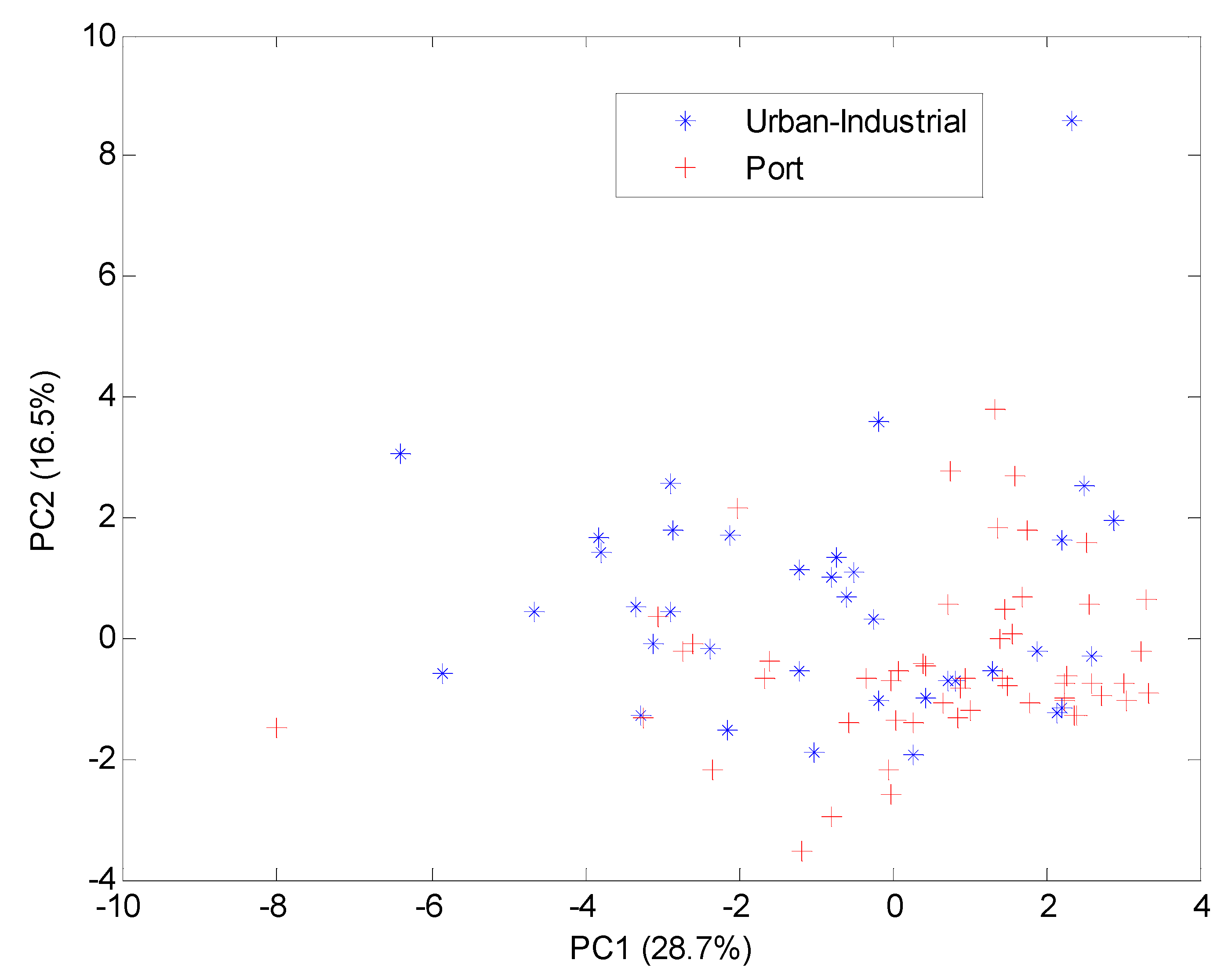
3.2. Principal Component Analysis

Before applying PCA, a preliminary analysis of data set was performed: 8 samples were excluded from it (6 samples characterized by Saharan Dust episode and 2 samples characterized by biomass burning) and the distribution of the variables was checked: some of them showed logarithmic distributions. For these variables logarithmic transformation was therefore applied to bring them closer to a normal distribution. Since PCA is sensible to the presence of outliers in the data matrix, Q index and T² Hoteling tests were applied to evaluate this presence. By the tests, one sample was identified as outlier and it was removed from the data matrix. Variables redundancy influences the efficiency of PCA method and complicates the results interpretation. For this reason, redundant variables such as TC, PM_2.5, K, Na, Ca, Mg, C₂O₄²⁻, etc. have been deleted from the data set before applying the PCA, and the final data set used was composed of 91 samples and 19 variables (Fe, V, Ni, Cu, Cr, Cd, Mn, Cl⁻, NO₃⁻, SO₄²⁻, Na⁺, NH₄⁺, K⁺, Mg²⁺, Ca²⁺, WSOC, WSIC, OC, EC).

Figure 3 shows the score plot in the plane of the first and second Principal Components (auto-scaled data), accounting for 45% of the total variance. The separation of samples between two prevalent wind directions is not totally clear. Blue samples (collected when the prevalent wind direction was from urban and industrial area) showed a slightly larger dispersion than the red ones. This is since different sources affected the sampling site [21] and the collected samples which are daily averages were affected by all sources. Perhaps in future campaigns wind selective sampling could be utilized to reduce meteorology related uncertainties.

Table 2. Principal Component Analysis (PCA) Loading values. Values larger than 0.23 are highlighted in bold.

	PC1	PC2	PC3	PC4	PC5	PC6	PC7
Fe	0.47	0.03	−0.11	0.08	0.01	−0.01	0.06
V	0.43	0.02	0.21	0.01	−0.15	−0.09	−0.02
Ni	0.38	−0.09	0.04	0.06	0.10	0.00	−0.32
Cu	0.10	−0.10	−0.03	0.62	0.08	0.02	−0.15
Pb	−0.06	−0.08	−0.01	−0.20	0.06	0.03	0.71
Cd	0.11	0.02	0.12	0.17	0.03	−0.02	0.44
Mn	0.44	0.04	−0.01	−0.08	0.06	0.06	0.06
OC	0.17	−0.06	−0.07	0.04	0.41	0.10	0.09
EC	0.21	−0.07	−0.16	0.38	0.02	−0.03	0.33
Cl−	−0.14	0.51	−0.10	0.19	0.02	−0.04	0.03
NO3−	−0.24	0.20	0.14	0.55	−0.13	0.02	0.11
SO4−	0.04	0.02	0.64	−0.06	0.06	0.00	0.02
Na+	0.07	0.65	0.00	−0.09	0.04	−0.10	−0.04
NH4+	−0.04	−0.06	0.66	0.07	−0.03	0.01	0.03
K+	0.03	0.16	0.04	−0.12	0.54	−0.07	0.09
Mg2+	0.16	0.46	0.07	−0.09	−0.04	0.25	−0.04
Ca2+	0.03	0.04	−0.01	0.01	0.09	0.62	0.04
WSOC	−0.20	−0.07	0.07	0.11	0.68	−0.01	−0.16
WSIC	−0.06	−0.05	0.00	0.01	−0.08	0.71	−0.04
Explained Variance (%)	28.7	16.5	10.3	8.3	6.9	5.3	4.9

shows the factor loading values of the considered parameters. All the factors which showed eigenvalue greater or equal to 1 have been considered. Seven factors (PCs) were evaluated, explaining up to 81% of the total variance. Factor loadings of the variables were used to identify source profiles affecting the investigated sampling site.

The first Principal Component (PC1) accounting for 29% of the total variance showed larger loading values for Fe, V, Ni and Mn, suggesting a mixed source, composed of ship emissions and crustal resuspension. The second PC, accounting for 17% of the total variance, showed high loading values for Cl⁻, Na⁺, and Mg²⁺, suggesting the presence of sea salt source. The third PC, accounting for 10% of the total variance, is characterized by higher loading values of SO₄²⁻ and NH₄⁺ and is associated to ammonium sulphate of secondary origin. The fourth PC, characterized by Cu, EC, and NO₃⁻, represents the contribution of vehicular traffic emissions accounting for 8% of the total variance. The fifth PC, characterized by K⁺, EC, and NO₃⁻, indicates a possible contribution from biomass combustions or fires to PM_2.5 concentration, with an explained total variance of 7%. The sixth PC is characterised by the species WSIC and Ca²⁺ (5% of the total variance) and it represents the contribution of calcium carbonate which is present in the crustal matter, re-suspended dust and particles from construction work. The seventh PC presents higher loadings of Pb, Cd, and EC with an explained variance of 5%, this factor suggests an industrial origin.

It is well known that both PCA and LDA are linear transformation techniques used for dimensionality reduction. PCA “ignores” class labels and its purpose is to find the directions (the principal components) that maximize the variance in a dataset, and it can be considered an “unsupervised” algorithm. In contrast to PCA, LDA is “supervised” and computes the directions (“linear discriminants”) that will represent the axes that maximize the separation between multiple classes. Generally, for a multi-class classification task where the class labels are known, LDA is considered a more robust technique. For this reason, LDA was applied to our data set.

3.3. Linear Discriminant Analysis

Table 3. Confusion matrix in cross validation and percentage of correct predictions.

	Urban-Industrial	Port	Correct Prediction (%)
Urban-Industrial	20	13	61
Port	10	48	83

shows the confusion matrix in cross validation (Venetian blind, 5 segments) and the percentage of correct predictions for data set obtained by LDA are shown. The overall percentage of correct predictions in cross validation is 72%.

By LDA it has been possible to point out the discreet separation between urban-industrial and port prevalent wind directions macroareas, that by PCA was just hinted. It is possible to observe that the model assigned samples to the category represented by Urban-Industrial with good percentage of correct predictions (61%), but it assigned samples to the category represented by Port with a high percentage of correct predictions, that is 83%: in fact, in this case, only 10 samples have been mispredicted on 58.

3.4. Mass Closure Analysis

Results on mass closure analysis (or mass reconstruction) are here reported to quantitatively identify the contribution of various emission sources on PM_2.5 samples, respectively, on the two prevailing directions identified and then confirmed by LDA. Mass reconstruction is defined by seven main classes (sources): sea-spray, crustal matter, secondary inorganic aerosol (SIA), secondary organic aerosol (SOA), combustion, anthropogenic metals, and the undefined mass (UM). The different calculations and hypotheses used for the aerosol mass reconstruction are reported below.

Sea-spray mass concentrations were calculated by adding to sodium, chloride, and the sea-salt (ss) contributions of calcium, potassium, and sulphate as follows:

Sea-spray = Na⁺ + Cl⁻ +ss-Mg²⁺ + ss-K⁺ + ss-Ca²⁺ + ss-SO₄²⁻

(1)

where ss-K⁺, ss-Ca²⁺, ss-Mg²⁺, and ss-SO₄²⁻ have been estimated as measured Na⁺ times 0.036, 0.038, 0.129, and 0.2516, respectively [57].

Crustal matter mass concentration estimate is based on Al, Si, Fe, and insoluble fraction (M_ins) of Na, K, Mg, and Ca. Due to the high correlation between Ca and WSIC, the presence of carbonates was assumed (0.72, p < 0.05) and the WSIC concentration was added to crustal matter. Then the crustal matter was calculated by the following equation assuming that Al and Fe are of crustal origin [58,59]:

Crustal matter = 21.67 * Mg_ins + 1.4 * Ca_ins + 1.35 * Na_ins + 1.43·Fe + 1.89 * Al + 2.14 * (Si/Al)_crust * Al + 1.2 * K_ins + WSIC

(2)

where (Si/Al)_crust is the ratios determined by Wedephol [60], and the insoluble fraction of Ca, Mg, K, and Na were calculated as follows:

M_ins = M_tot- Mⁿ⁺

(3)

Secondary inorganic aerosol (SIA) mass concentrations were calculated as:

SIA = (nss-SO₄²⁻ + NO₃⁻ + NH₄⁺)·1.29

(4)

where 1.29 is the factor to convert the inorganic species into hydrated species.

Secondary organic aerosol (SOA) mass concentrations were calculated from OC_sec mass concentrations as:

SOA = f_OM/OCOC_sec

(5)

where f_OM/OC = 2.1 for samples collected with prevalent wind from port direction and f_OM/OC = 1.8 when winds blew from urban-industrial area [61]. Moreover, the EC-tracer method was employed to derive OC_sec from the EC [62].

Combustion mass concentration was calculated as follows:

Combustion = nss-K⁺ + EC + OC_prim·f_OM/OC

(6)

where nss-K⁺ has been calculated as:

nss-K⁺ = K⁺-ssK⁺

(7)

Table 4. Mean mass concentration (µg m⁻³) and standard deviation of PM_2.5 and of the main mass classes: secondary inorganic aerosol (SIA), secondary organic aerosol (SOA), combustion, crustal matter, anthropogenic metals, sea salt, and the undefined mass (UM).

µg m−3	PM2.5	SIA	SOA	Combustion	Crustal Matter	Anthropogenic Metals	Sea Salt	Undef.
Urban-Industrial	17 ± 6	6.2 ± 1.6	3.1 ± 1.2	3.3 ± 0.2	3 ± 2	0.040 ± 0.019	0.6 ± 0.2	0.3 ± 0.4
Port	14 ± 5	5.5 ± 1.6	2.4 ± 0.9	2.4 ± 0.2	3 ± 2	0.031 ± 0.025	0.5 ± 0.2	0.2 ± 0.3

shows the mean mass concentrations of the six main sources considered for the mean mass reconstruction of the PM_2.5 fraction. For both prevailing wind directions, the unexplained mass was low, that is 1.8% and 1.6% for urban-industrial direction and port direction, respectively. Moreover, considering that the particulate mass (PM_2.5 mass) was higher for samples of urban-industrial area direction, the SIA, SOA, combustion, and crustal fractions were present in larger amounts when winds blew from this area, while the sea salt contribution was not statistically different between the two directions. It is also clear that notwithstanding the amount of SIA was lower in the port direction, it represented higher load on the PM_2.5 mass: 40.1% for port direction, 36.8% for urban-industrial direction.

3.5. Modelling Results

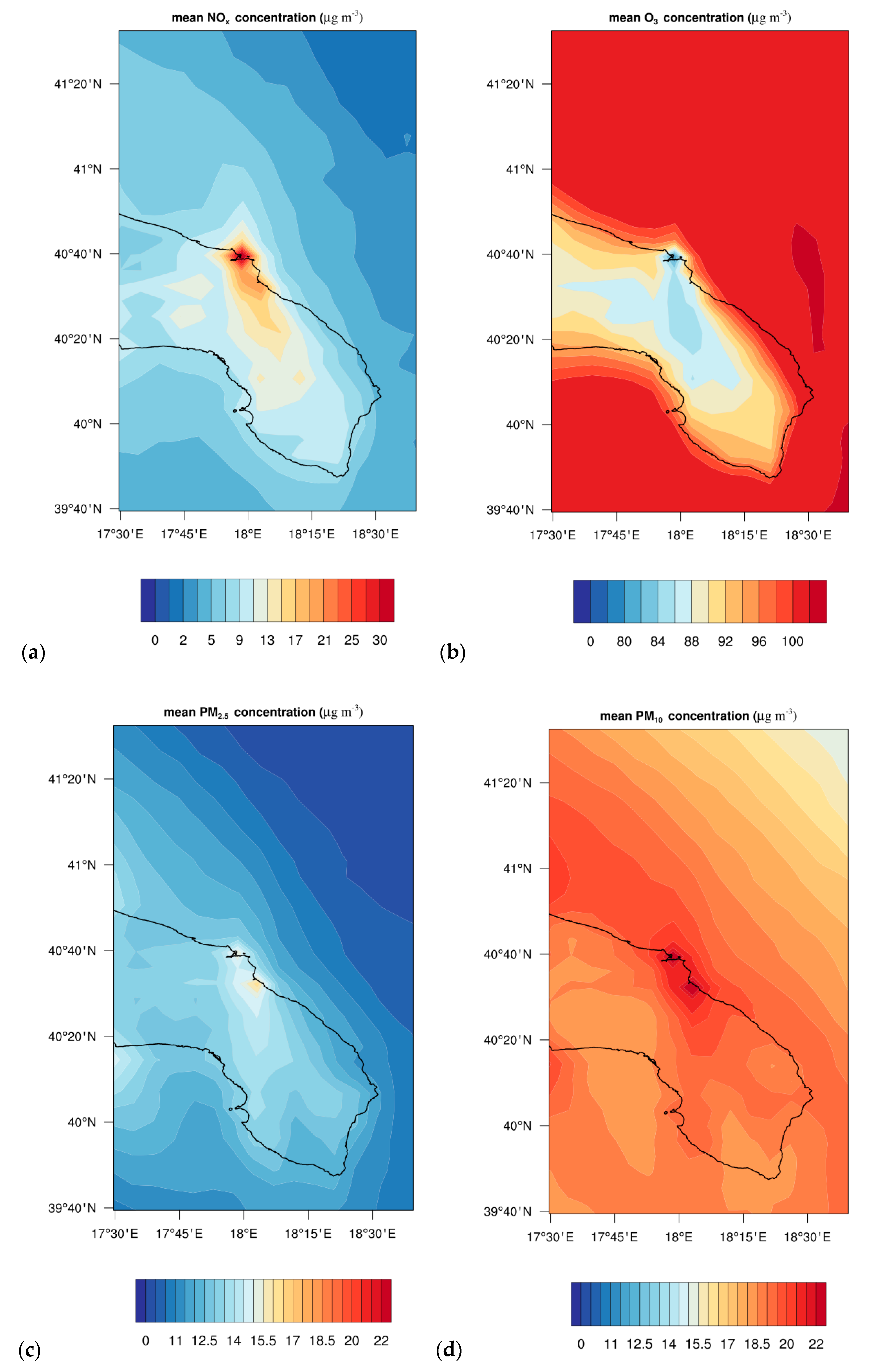
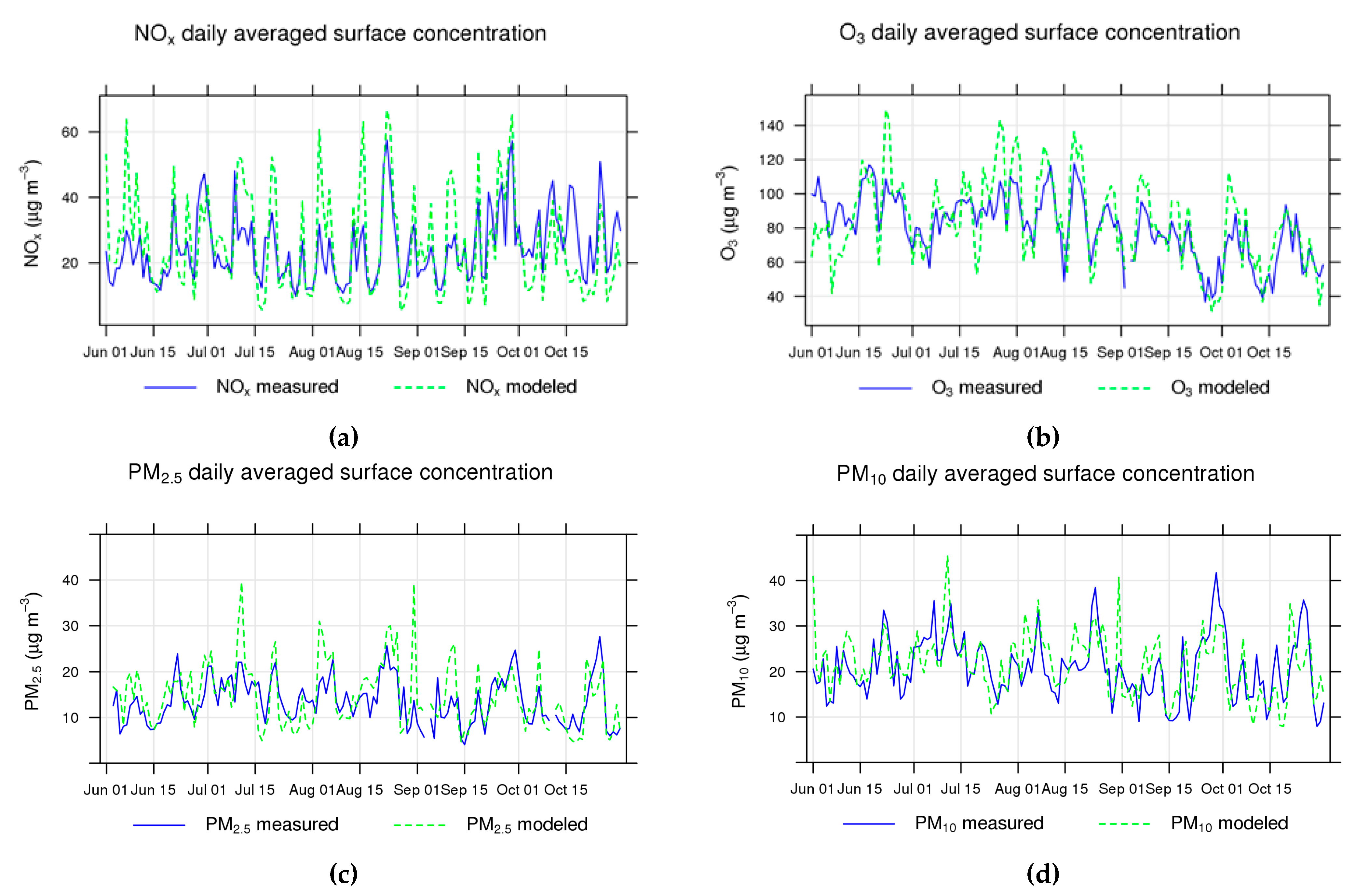
3.5.1. Pollutant Concentration Levels in the Study Area

BOLCHEM was first used to evaluate the air quality in the study area for the measurement campaign period (June–October 2012). Figure 4 shows the spatial distribution of NO_X, O₃, PM_2.5 and PM₁₀ ground concentrations averaged over the whole period. The ability of BOLCHEM was verified against data from the measurement campaign (available only for PM_2.5) and data of monitoring stations managed by ARPA-Puglia. Figure 5 shows the time series of modelled and measured daily averaged concentration over the whole period. To quantify the model performance, the Pearson correlation coefficient (R), the mean bias (MB) and the root mean square error (RMSE) were also calculated. In the calculation of the statistical indicators, mean daily value of modelled and observed data were used. The mean concentration averaged over the whole period, in addition to the statistical indices, are reported in

Table 5. BOLCHEM modelled and measured concentrations (µg m⁻³) averaged over ARPA-Puglia and ASI monitoring stations and over the whole period June–October 2012.

	Modelled (µg m−3)	Measured (µg m−3)	MB (µg m−3)	RMSE (µg m−3)	R
NOX	25.61	24.68	0.93	11.17	0.68
O3	83.54	79.71	3.83	16.19	0.78
PM2.5	14.91	13.59	1.32	5.69	0.64
PM10	21.53	20.85	0.68	5.97	0.61

.

BOLCHEM overestimation of NO_X can be due to the fact that output refers to the model cell representing the port, where also ship emissions are located, as well as to the uncertainty of the employed emissions inventory (see Section 2.4.1). As for PM_2.5 and PM₁₀, they showed an overestimation probably due to the overestimation of sea salt by the model, while Saharan dust events occurred at the end of September and October were not reproduced by the model. However, since the focus is on the impact of ship emissions, we expect such overestimations slightly affected the results.

Results show that BOLCHEM acceptably agreed with measured data. The model was then used in combination with ADMS-Urban to estimate the contribution of ship emissions on pollutant concentration levels following the zero-out method.

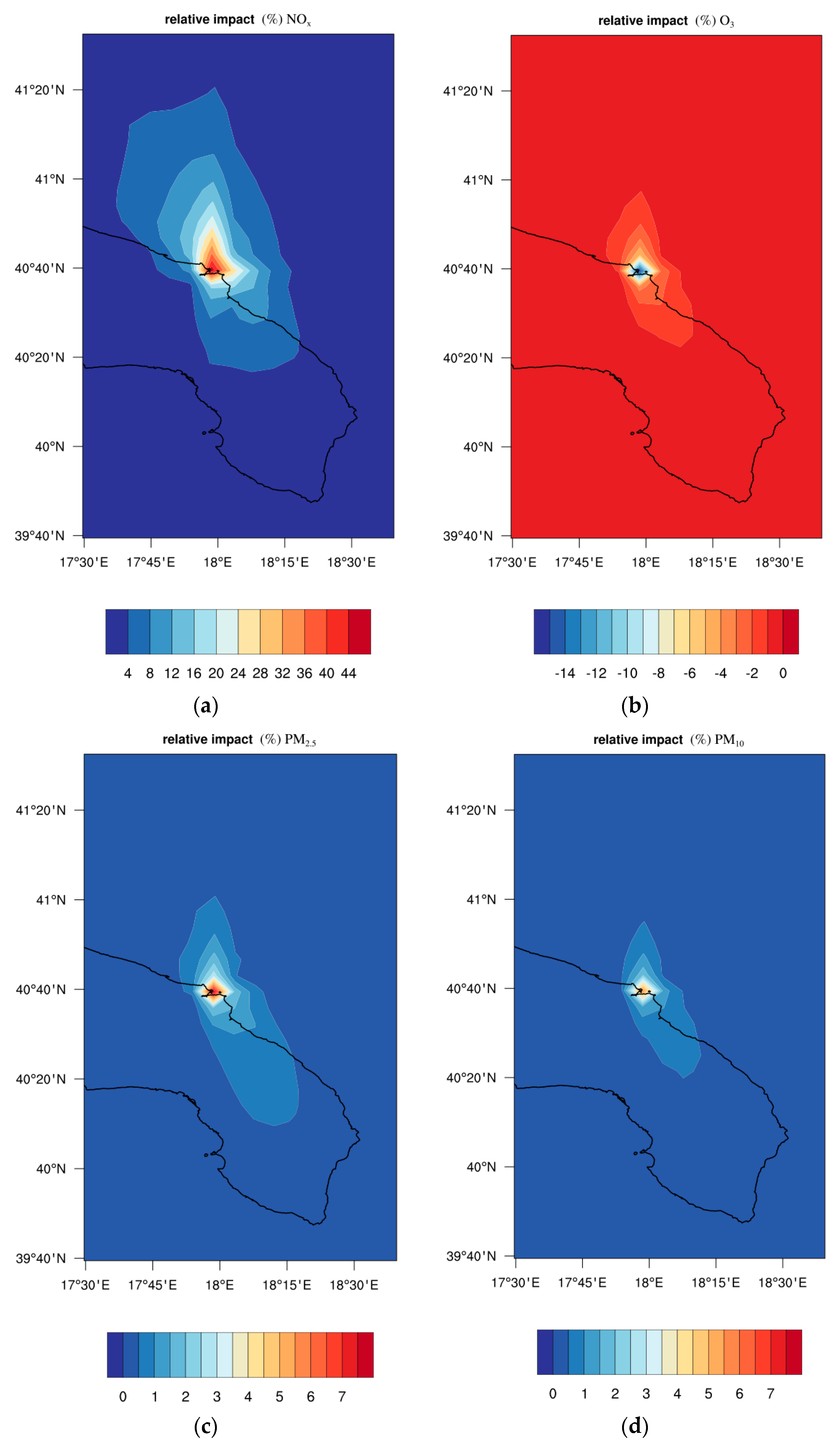
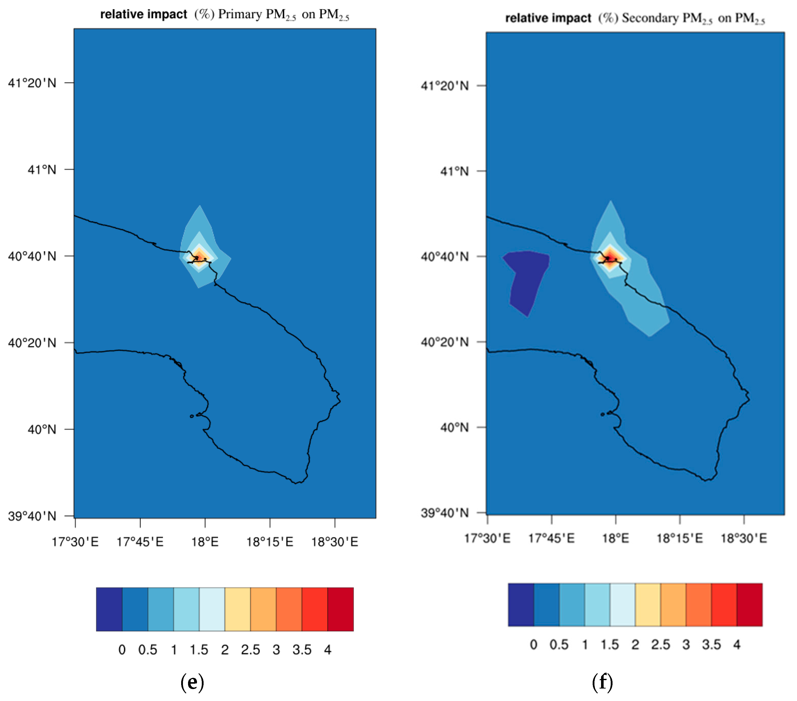
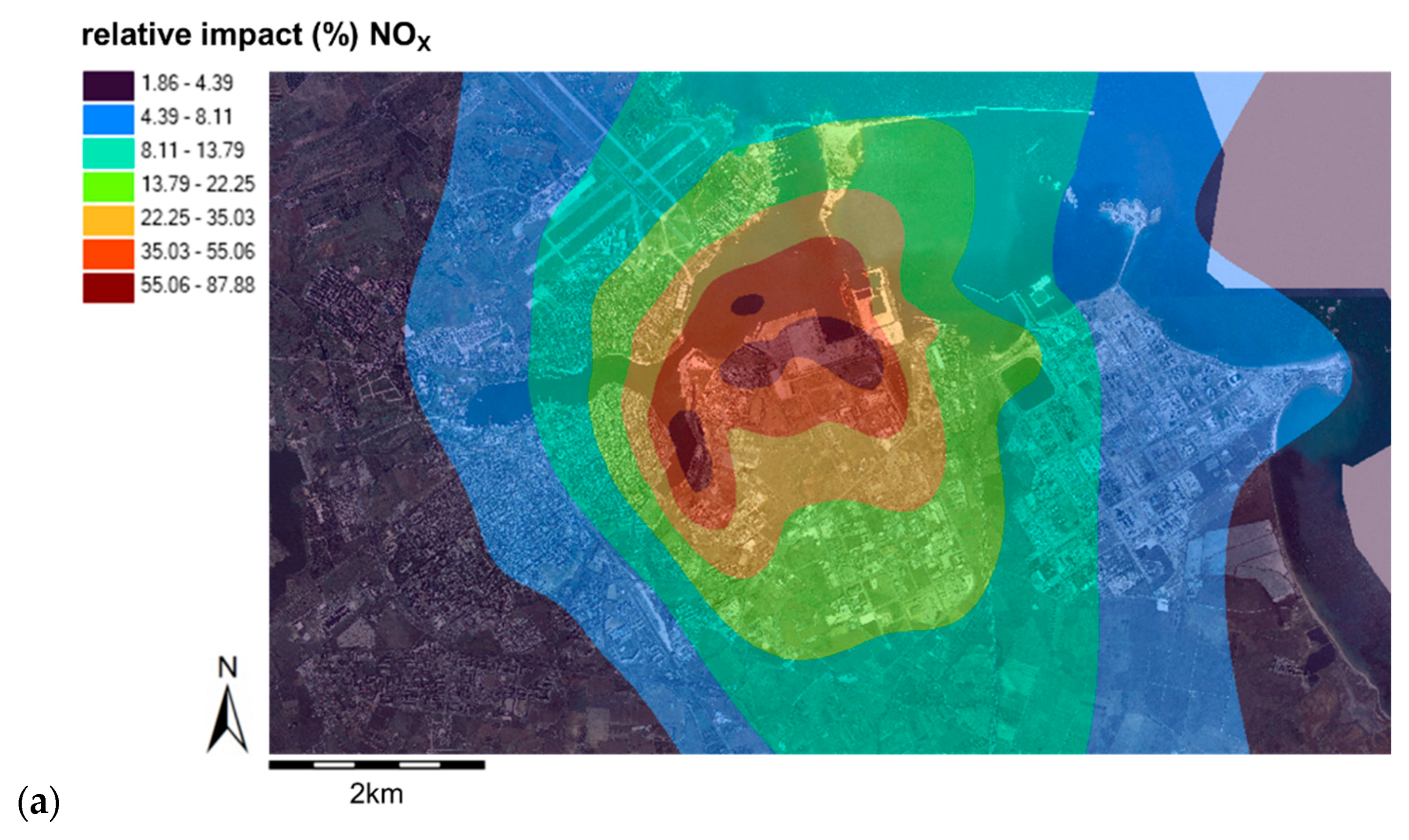
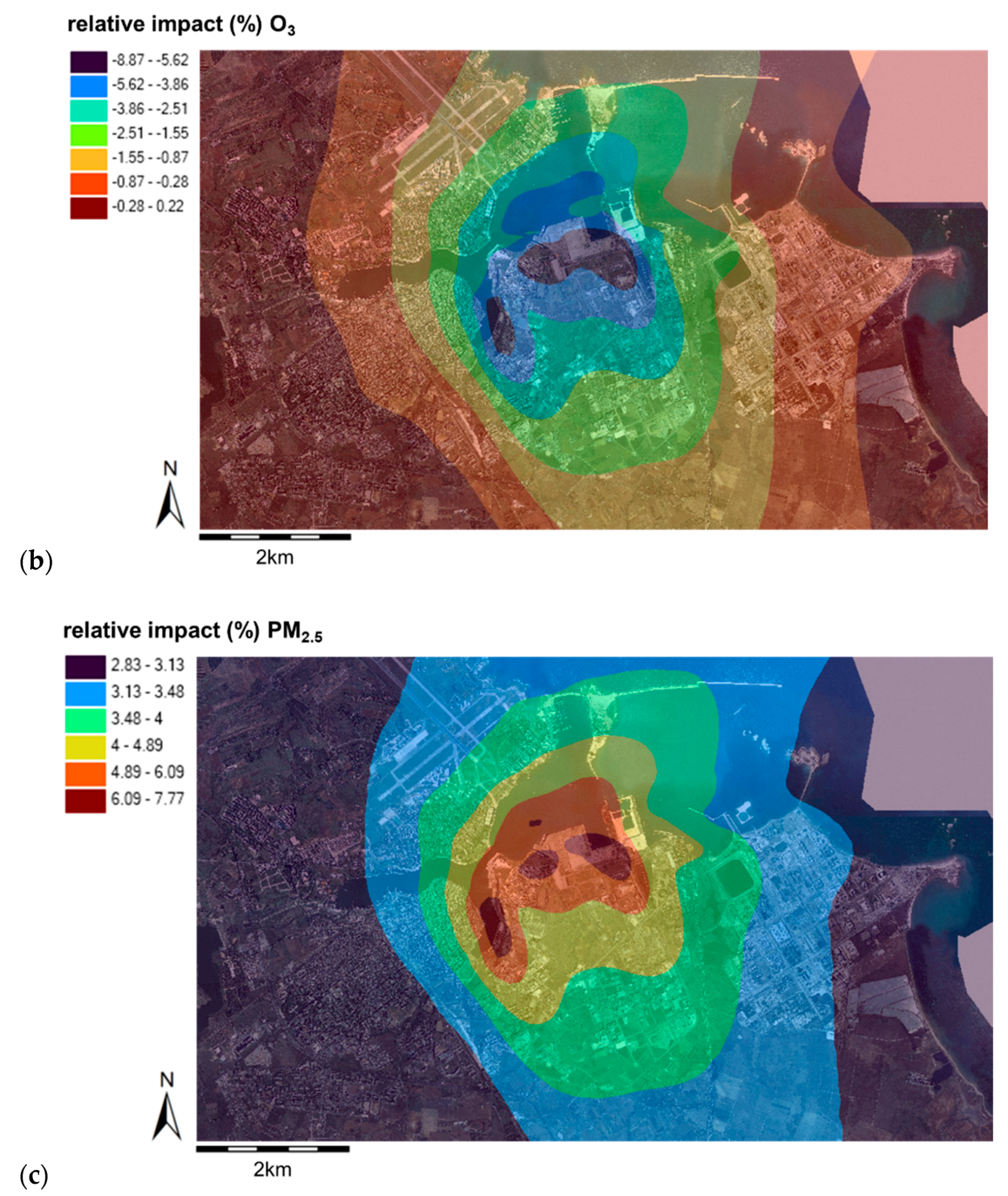
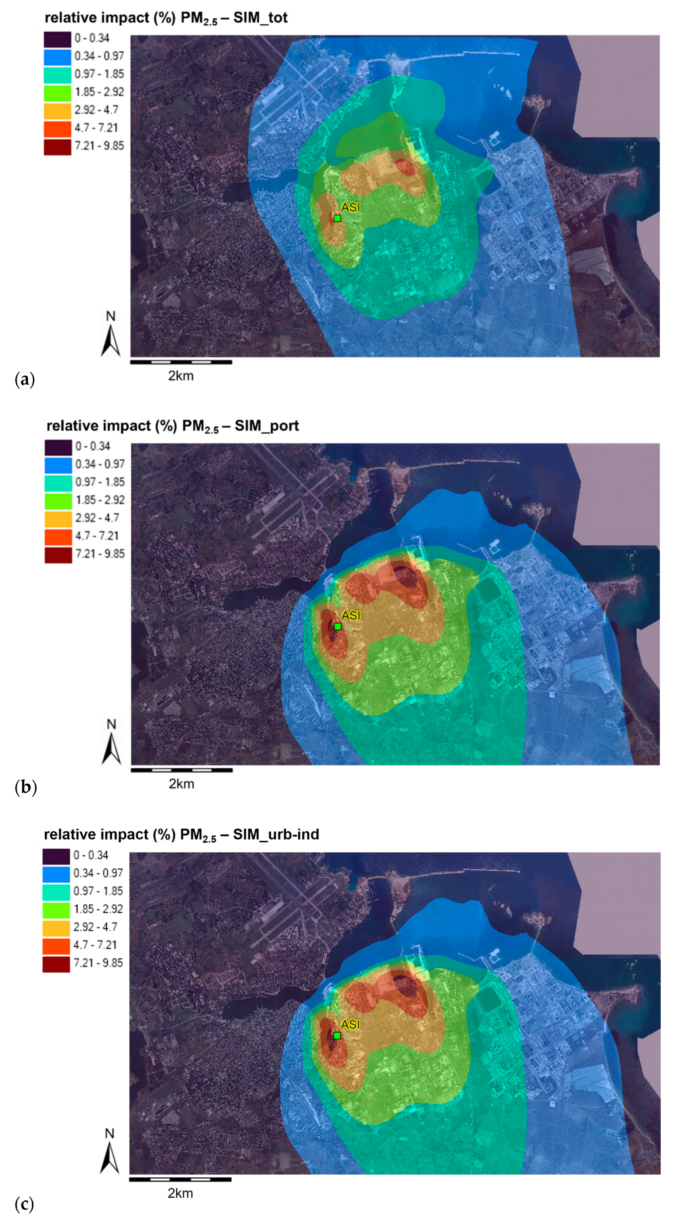
3.5.2. Ship Emissions Impact

The ship emissions impact on NO_X, O₃, PM_2.5, and PM₁₀ has been evaluated using both BOLCHEM and ADMS-Urban. The impact was calculated as (C_{with_ships} − C_{no_ships})/C_{with_ships}, with C the average concentration over the simulation period, C_{with_ships} the concentration calculated with the inclusion of ship emissions, C_{no_ships} that calculated without ship emissions (which is the concentration employed as background in ADMS-Urban simulations).

Figure 6 shows the relative impact on NO_X, O₃, PM_2.5, and PM₁₀ ground concentration obtained from BOLCHEM, while Figure 7 shows the relative impact obtained from ADMS-Urban at 2 m. As regards gas species, both figures show that, due to ship emissions, NO_X concentration increased in the port area, while O₃ decreased due to enhanced titration caused by NO_X emissions.

Table 6. BOLCHEM estimated impact of ship emissions pollutant concentrations in the port area.

BOLCHEM	% Impact
NOX	37.6
O3	−11.7
Primary PM2.5	2.7
Secondary PM2.5	3.4
PM2.5	6.1
PM10	4.3

summarizes the impact obtained from BOLCHEM in the port area. In the cell of the port, the estimated ship emissions contribution was 6.1% for PM_2.5 and 4.3% for PM₁₀. For PM_2.5, the contribution of the primary component was 2.7%. These results are comparable with results found by Cesari et al. [21] (2.8% ± 1.1%) and Donateo et al. [22] (7.4% ± 0.5%) for the same port at the ASI sampling site. The secondary contribution to PM_2.5 (3.4%) was lower of that estimated in Cesari et al. [21], who found a contribution of secondary ammonium sulphate of about 11% of PM_2.5. This can be due to the different used approach [29]. We also recall the strong dependence of model results on model formulation [26,27] and applied inventory [25], whose structure identifies the source in the CTMs model [29]. As for NO_X and O_3, the impact on NO_X concentration was 37.6%, with a corresponding decrease of 11.7% on O₃ concentration. ADMS-Urban, although the simplified chemical scheme, showed values consistent with BOLCHEM results. Further, it allowed to investigate the spatial distribution showing maximum located in the hotelling areas. We recall that the net formation of O₃ depends on the levels of NO_X and NMVOC, as well as their ratio. In regions with high NO_X concentrations, O₃ production is limited by the availability of NMVOC, while in areas limited by the availability of NO_X, an increase in NO_X emissions will lead to an increase of O₃ production [13,63]. The decrease of O₃ concentration corresponding to an increase of NO_X emissions is in accordance with the fact that although the Italian peninsula is almost entirely NO_X-sensitive, there are well defined VOC-sensitive regions located over urban/industrial areas and harbours [64]. In such polluted area, O₃ production is more sensitive to VOC emissions, and then it decreases with increasing NO_X emissions. In the same area, Merico et al. [65] found a similar O₃ decrease (about 5%). Model simulations of the effects of global ship emissions on European domain [13] found that the effect of reducing ship emission in the Mediterranean Sea was a widespread O₃ titration close to major shipping lanes and harbour, especially in winter. During spring and summer, an increase of O₃ was found in the South-Eastern Mediterranean Sea.

ADMS-Urban was finally employed to evaluate the spatial distribution of ship-related concentrations of PM_2.5. The simulations were performed considering periods according to the two observed prevailing wind directions (see Section 2.1) based on the analysis of the measured data to facilitate the comparison between simulated concentration and findings derived from chemical characterization. Three different sets of simulations were performed:

• prevailing winds from northern sectors (SIM_port hereinafter);
• prevailing wind from southern sectors (SIM_urb-ind hereinafter);
• finally, SIM_tot refers to the period comprising all the days considered in the previous two simulations.

Averaged concentration of PM_2.5 measured and simulated at ASI position have been compared for the three set of simulations.

Table 7. ADMS-Urban modelled and measured averaged PM_2.5 concentrations (µg m⁻³) at sampling site (ASI) position, and modelled impact of ship emissions (%).

	Modelled PM2.5 (µg m−3)	Measured PM2.5 (µg m−3)	Modelled Impact (%)
SIM_tot	14.0	16 ± 6	4.2
SIM_port	12.9	14 ± 5	6.8
SIM_urb-ind	16.8	17 ± 6	0.9

shows that modelled results agreed with measurements given that both shows larger concentration in the SIM_urb-ind case. However, simulations slightly underestimated measured concentrations probably due to different reasons. Emissions related to port activity (loading/unloading phase) and chemical reactions regarding secondary PM were not included in ADMS-Urban. Furthermore, the contribution of urban and industrial emissions was considered as background concentrations obtained from BOLCHEM and thus not explicitly reproduced. The impact at ASI position has been evaluated for the three sets of simulations and was 4.2% for the SIM_tot, 6.8% for the SIM_port, and 0.9% for SIM_urb-ind. The impact is in the range between values estimated by Cesari et al. [21] and Donateo et al. [22] for the same port at the same sampling site.

Figure 8 finally synthesises the spatial impact of port emissions on the whole study area showed in % at 2 m for the three sets of simulations. Mean concentration distribution follows the prevailing wind direction with a decrease far away from the sources. Overall, Figure 8a shows the largest impact was located in the hotelling area. Figure 8b,c show that, when the prevailing winds were from southern sectors (SIM_urb-ind), the impact of the port emissions was localized within the port, while when the winds were from northern sectors (SIM_port) the impact of port was larger and confined in the urban area downwind to the sources up to a distance of about 2 km, after that it reduces to lower than 3%.

4. Summary and Conclusions

This paper combines measurements and modelling approaches to investigate the air quality and the impact of ship emissions on NO_X, O₃, and PM in a Mediterranean port city (Brindisi, Apulia Region, Southern Italy).

As for measurements, 100 daily samples of fine PM were collected on the roof of the ASI building during a field experimental campaign. The PM_2.5 samples were chemically characterized in terms of ionic fraction, carbonaceous components and metals. A statistical analysis was conducted integrating complementary tools, LDA and PCA. PCA was useful to examine data structure in terms of the main sources which in this case were crustal and ship emissions (29% of the total variance), sea spray (17% of the total variance), combustion (7% of the total variance), vehicular traffic (8%), industrial (5%), and secondary aerosol (10%). By PCA no statistical differentiation of samples for the two prevailing wind directions was obtained. Probably, more useful information could be obtained using wind selective samplers. The application of LDA was successful in separating the contribution between prevalent wind directions associated to the main contributing sources: the method assigned samples to the category ‘Urban-Industrial’ with good percentage of correct predictions (61%), and samples to the category ‘Port’ with a high percentage of correct predictions (83%), respectively.

Then, the air quality and the direct impact of ship emissions contribution during the experimental period were quantified by employing a numerical modelling system (coupling offline the mesoscale chemistry model BOLCHEM and the local scale dispersion model ADMS-Urban). BOLCHEM simulations were performed to reproduce ground pollutants concentrations and the impact of ship-related PM emissions on PM_2.5 and PM₁₀ concentrations, as well as of NO_X and NMVOC emissions on NO_X and O₃ concentration, at a regional scale. The spatial distribution of concentration levels at local scale has been then assessed using ADMS-Urban. BOLCHEM results showed that the impact of ship emissions covered an area of a few dozen kilometers and was, on average for the field experimental campaign period, 37.6% for NO_X, −11.7% for O₃, 4.3% for PM₁₀, and 6.1% for PM_2.5, the last one distributed between primary (2.7%) and secondary fraction (3.4%). At a local scale, the analysis of high-resolution modelling results obtained from ADMS-Urban highlighted that, at ASI position, the impact of ship emissions on PM_2.5 was 6.8% when the sampling site was positioned downwind to the port area and reduced to lower than 3.0% at about 2 km far from the sources.

This study is an example of integrated methodologies which could be further tested in other port cities which could have even larger complexity than in our case in terms of sources, topographic features, and in turns of meteorological processes.

References

1. Mangia, C.; Ielpo, P.; Cesari, R.; Facchini, C. Crisi climatica e inquinamento atmosferico. Ithaca Viaggio Nella Scienza 2020, 15, 1–11. [Google Scholar]
2. Von Schneidemesser, E.; Monks, P.S.; Allan, J.D.; Bruhwiler, L.; Forster, P.; Fowler, D.; Lauer, A. Chemistry and the linkages between air quality and climate change. Chem. Rev. 2015, 115, 3856–3897. [Google Scholar] [CrossRef]
3. Leibensperger, E.M.; Mickley, L.J.; Jacob, D.J.; Kumar, N.; Rind, D. Climatic effects of 1950-2050 changes in US anthropogenic aerosols-Part 1: Aerosol trends and radiative forcing. Atmos. Chem. Phys. 2012, 12, 3333–3348. [Google Scholar] [CrossRef] [Green Version]
4. Leibensperger, E.M.; Mickley, L.J.; Jacob, D.J.; Kumar, N.; Rind, D. Climatic effects of 1950-2050 changes in US anthropogenic aerosols-Part 2: Climate response. Atmos. Chem. Phys. 2012, 12, 3349–3362. [Google Scholar] [CrossRef] [Green Version]
5. Karanasiou, A.; Querol, X.; Alastuey, A.; Perez, N.; Pey, J.; Perrino, C.; Berti, G.; Gandini, M.; Poluzzi, V.; the MED-PARTICLES Study Group; et al. Particulate matter and gaseous pollutants in the Mediterranean Basin: Results from the MED-PARTICLES project. Sci. Tot. Environ. 2014, 488–490, 297–315. [Google Scholar] [CrossRef] [PubMed]
6. Gaisbauer, S.; Wankmüller, R.; Matthews, B.; Mareckova, K.; Schindlbacher, S.; Tista, M.; Ullrich, B. Emissions for 2017. In Transboundary Particulate Matter, Photo-Oxidants, Acidifying and Eutrophying Components; EMEP Status Report 1/2019; The Norwegian Meteorological Institute: Oslo, Norway, 2017; pp. 43–64. Available online: https://emep.int/publ/reports/2019/EMEP_Status_Report_1_2019.pdf (accessed on 1 December 2020).
7. Eyring, V.; Isaksen, I.S.A.; Berntsen, T.; Collins, W.J.; Corbett, J.J.; Endresen, O.; Grainger, R.G.; Moldanova, J.; Schlager, H.; Stevenson, D.S. Transport impacts on atmosphere and climate: Shipping. Atmos. Environ. 2010, 44, 4735–4771. [Google Scholar] [CrossRef]
8. Viana, M.; Hammingh, P.; Colette, A.; Querol, X.; Degraeuwe, B.; de Vlieger, I.; van Aardenne, J. Impact of maritime transport emissions on coastal air quality in Europe. Atmos. Environ. 2014, 90, 96–105. [Google Scholar] [CrossRef]
9. Monteiro, A.; Russo, M.; Gama, C.; Borrego, C. How important are maritime emissions for the air quality: At European and national scale. Environ. Pollut. 2018, 242, 565–575. [Google Scholar] [CrossRef]
10. Jonson, J.; Gauss, M.; Schulz, M.; Nyíri, A. Emissions from international shipping. In Transboundary Particulate Matter, Photo-oxidants, Acidifying and Eutrophying Components; EMEP Status Report 1/2018; The Norwegian Meteorological Institute: Oslo, Norway, 2018; pp. 83–98. Available online: https://emep.int/publ/reports/2018/EMEP_Status_Report_1_2018.pdf (accessed on 1 December 2020).
11. Jonson, J.; Gauss, M.; Schulz, M.; Jalkanen, J.-P.; Fagerli, H. Effects of global ship emissions on European air pollution levels. Atmos. Chem. Phys. 2020, 20, 11399–11422. [Google Scholar] [CrossRef]
12. Marmer, E.; Langmann, B. Impact of ship emissions on the Mediterranean summertime pollution and climate: A regional model study. Atmos. Environ. 2005, 39, 4659–4669. [Google Scholar] [CrossRef]
13. Tagaris, E.; Stergiou, I.; Sotiropoulou, R.-E.P. Impact of shipping emissions on ozone levels over Europe: Assessing the relative importance of the Standard Nomenclature for Air Pollution (SNAP) categories. Environ. Sci. Pollut. Res. 2017, 24, 14903–14909. [Google Scholar] [CrossRef] [PubMed]
14. Eyring, V.; Stevenson, D.S.; Lauer, A.; Dentener, F.J.; Butler, T.; Collins, W.J.; Ellingsen, K.; Gauss, M.; Hauglustaine, D.A.; Isaksen, I.S.A.; et al. Multi-model simulations of the impact of international shipping on Atmospheric Chemistry and Climate in 2000 and 2030. Atmos. Chem. Phys. 2007, 7, 757–780. [Google Scholar] [CrossRef] [Green Version]
15. Sofiev, M.; Winebrake, J.J.; Johansson, L.; Carr, E.W.; Prank, M.; Soares, J.; Vira, J.; Kouznetsov, R.; Jalkanen, J.-P.; Corbett, J.J. Cleaner fuels for ships provide public health benefits with climate tradeoffs. Nature 2018, 9, 406. [Google Scholar] [CrossRef] [PubMed] [Green Version]
16. Schinas, O.; Stefanakos, C.N. Cost assessment of environmental regulation and options for marine operators. Transp. Res. Part C Emerg. Technol. 2012, 25, 81–99. [Google Scholar] [CrossRef]
17. Yang, Z.L.; Zhang, D.; Caglayan, O.; Jenkinson, I.D.; Bonsall, S.; Wang, J.; Huang, M.; Yan, X.P. Selection of techniques for reducing shipping NOx and SOx emissions. Transp. Res. D Transp. Environ. 2012, 17, 478–486. [Google Scholar] [CrossRef]
18. Sorte, S.; Rodrigues, V.; Borrego, C.; Monteiro, A. Impact of harbour activities on local air quality: A review. Environ. Pollut. 2020, 257, 113542. [Google Scholar] [CrossRef]
19. Schembari, C.; Cavalli, F.; Cuccia, E.; Hjorth, J.; Calzolai, G.; Perez, N.; Pey, J.; Prati, P.; Raes, F. Impact of a European directive on ship emissions on air quality in Mediterranean harbours. Atmos. Environ. 2012, 61, 661–669. [Google Scholar] [CrossRef]
20. Buccolieri, R.; Cesari, R.; Dinoi, A.; Maurizi, A.; Tampieri, F.; Di Sabatino, S. Impact of ship emissions on local air quality in a Mediterranean city’s harbour after the European Sulphur directive. Int. J. Environ. Pollut. 2016, 29, 30–42. [Google Scholar] [CrossRef]
21. Cesari, D.; Genga, A.; Ielpo, P.; Siciliano, M.; Mascolo, G.; Grasso, F.M.; Contini, D. Source apportionment of PM2.5 in the harbour-industrial area of Brindisi (Italy): Identification and estimation of the contribution of in-port ship emissions. Sci. Tot. Environ. 2014, 497, 392–400. [Google Scholar] [CrossRef]
22. Donateo, A.; Gregoris, E.; Gambaro, A.; Merico, E.; Giua, R.; Nocioni, A.; Contini, D. Contribution of harbour activities and ship traffic to PM2.5, particle number concentrations and PAHs in a port city of the Mediterranean Sea (Italy). Environ. Sci. Pollut. Res. 2015, 21, 9415–9429. [Google Scholar] [CrossRef]
23. Belis, C.A.; Karagulian, F.; Larsen, B.R.; Hopke, P.K. Critical review and meta-analysis of ambient particulate matter source apportionment using receptor models in Europe. Atmos. Environ. 2013, 69, 94–108. [Google Scholar] [CrossRef]
24. Belis, C.A.; Pernigotti, D.; Karagulian, F.; Pirovano, G.; Larsen, B.R.; Gerboles, M.; Hopke, P.K. A new methodology to assess the performance and uncertainty of source apportionment models in intercomparison exercises. Atmos. Environ. 2015, 119, 35–44. [Google Scholar] [CrossRef]
25. Seigneur, C. Current status of air quality models for particulate matter. J. Air Waste Manag. Assoc. 2001, 51, 1508–1521. [Google Scholar] [CrossRef] [PubMed] [Green Version]
26. Pirovano, G.; Balzarini, A.; Bessagnet, B.; Emery, C.; Kallos, G.; Meleux, F.; Mitsakou, C.; Nopmongcol, U.; Riva, G.M.; Yarwood, G. Investigating impacts of chemistry and transport model formulation on model performance at European scale. Atmos. Environ. 2012, 53, 93–109. [Google Scholar] [CrossRef]
27. Marmer, E.; Dentener, F.; Aardenne, J.; Cavalli, F.; Vignati, E.; Velchev, K.; Hjorth, J.; Boersma, F.; Raes, F. What can we learn about ship emission inventories from measurements of air pollutants over the Mediterranean Sea. Atmos. Chem. Phys. 2009, 9, 6815–6831. [Google Scholar] [CrossRef] [Green Version]
28. Zhang, Y.; Vijayaraghavan, K.; Seigneur, C. Evaluation of three probing techniques in a three-dimensional air quality model. J. Geophys. Res. 2005, 110, D02305. [Google Scholar] [CrossRef] [Green Version]
29. Bove, M.C.; Brotto, P.; Cassola, F.; Cuccia, E.; Massabò, D.; Mazzinoa, A.; Piazzalunga, A.; Prati, P. An integrated PM2.5 source apportionment study: Positive matrix factorisation vs. the chemical transport model CAMx. Atmos. Environ. 2014, 94, 274–286. [Google Scholar] [CrossRef]
30. Putaud, J.P.; Van Dingenen, R.; Alastuey, A.; Bauer, H.; Birmili, W.; Cyrys, J.; Flentje, H. A European aerosol phenomenology-3: Physical and chemical characteristics of particulate matter from 60 rural, urban, and kerbside sites across Europe. Atmos. Environ. 2010, 44, 1308–1320. [Google Scholar] [CrossRef]
31. Mircea, M.; D’Isidoro, M.; Maurizi, A.; Vitali, L.; Conforti, F.; Zanini, G.; Tampieri, F. A comprehensive performance evaluation of the air quality model BOLCHEM to reproduce the ozone concentrations over Italy. Atmos. Environ. 2008, 42, 1169–1185. [Google Scholar] [CrossRef]
32. Cesari, R.; Landi, T.C.; D’Isidoro, M.; Mircea, M.; Russo, F.; Malguzzi, P.; Tampieri, F.; Maurizi, A. The On-Line Integrated Mesoscale Chemistry Model BOLCHEM. Atmosphere 2021, 12, 192. [Google Scholar] [CrossRef]
33. CERC ADMS-Urban User Guide. 2020. Available online: http://cerc.co.uk/environmental-software/assets/data/doc_userguides/CERC_ADMS-Urban5.0_User_Guide.pdf (accessed on 9 November 2020).
34. Birch, M.E.; Cary, R.A. Elemental carbon-based method for monitoring occupational exposures to particulate diesel exhaust. Aerosol. Sci. Technol. 1996, 25, 221–241. [Google Scholar] [CrossRef]
35. Cassinelli, M.E.; O’Connor, P.F. (Eds.) NIOSH: Method 5040. In NIOSH: Manual of Analytical Methods (NMAM), 4th ed.; 1998; Suppl. 2, Supplement to DHHS (NIOSH) Publication No. 94-113. Available online: https://www.cdc.gov/niosh/docs/2014-151/pdfs/methods/5040.pdf (accessed on 1 March 2021).
36. Scerri, M.M.; Genga, A.; Iacobellis, S.; Delmaire, G.; Give, A.; Siciliano, M.; Siciliano, T.; Weinbruch, S. Investigating the plausibility of a PMF source apportionment solution derived using a small dataset: A case study from a receptor in a rural site in Apulia—South East Italy. Chemosphere 2019, 236, 124376. [Google Scholar] [CrossRef] [PubMed]
37. Siciliano, T.; Siciliano, M.; Malitesta, C.; Proto, A.; Cucciniello, R.; Give, A.; Iacobellis, S.; Genga, A. Carbonaceous PM10 and PM2.5 and secondary organic aerosol in a coastal rural site near Brindisi (Southern Italy). Environ. Sci. Pollut. Res. 2018, 25, 23929–23945. [Google Scholar] [CrossRef] [PubMed]
38. Thurston, G.D.; Spengler, J.D. A quantitative assessment of source contributions to inhalable particulate matter pollution in metropolitan Boston. Atmos. Environ. 1985, 19, 9–25. [Google Scholar] [CrossRef]
39. Brereton, R.G. Applied Chemometrics for Scientists; John Wiley & Sons Ltd.: Hoboken, NJ, USA, 2007. [Google Scholar]
40. Belis, C.A.; Larsen, B.R.; Amato, F.; Haddad, I.E.; Favez, O.; Harrison, R.M.; Hopke, P.K.; Nava, S.; Paatero, P.; Prévôt, A.; et al. European Guide on Air Pollution Source Apportionment with Receptor Models; Report EUR 26080 EN; Publications Office of the European Union: Luxembourg, 2014. [Google Scholar]
41. Rencher, A.C. Methods of Multivariate Analysis; John Wiley & Sons Ltd.: Hoboken, NJ, USA, 2002. [Google Scholar]
42. Ielpo, P.; Leardi, R.; Pappagallo, G.; Uricchio, V.F. Tools based on multivariate statistical analysis for classification of soil and groundwater in Apulian agricultural sites. Environ. Sci. Pollut. Res. 2016, 24, 13967–13978. [Google Scholar] [CrossRef] [PubMed]
43. EEA/EMEP Air pollutant Emission Inventory Guidebook, Technical Report No 12/2013. Available online: https://www.eea.europa.eu/publications/emep-eea-guidebook-2013/at_download/file (accessed on 9 November 2020).
44. Buzzi, A.; Fantini, M.; Malaguzzi, P.; Nerozzi, P. Validation of a limited area model in cases of Mediterranean cyclogenesis: Surface fields and precipitation scores. Meteorol. Atmos. Phys. 1994, 53, 37153. [Google Scholar] [CrossRef]
45. Carter, W.A. detailed mechanism for the gas phase atmospheric reactions of organic compounds. Atmos. Environ. 1990, 27A, 481518. [Google Scholar] [CrossRef]
46. Silibello, C.; Calori, G.; Brusasca, G.; Giudici, A.; Angelino, E.; Fossati, G.; Peroni, E.; Buganza, E. Modelling of PM10 concentrations over Milano urban area using two aerosol modules. Environ. Model. Softw. 2008, 23, 333343. [Google Scholar] [CrossRef]
47. Binkowski, F.S.; Roselle, S.J. Models-3 Community Multiscale Air Quality (CMAQ) model aerosol component 1. Model description. J. Geophys. Res. 2003, 108 D6, 4183. [Google Scholar] [CrossRef]
48. Nenes, A.; Pandis, S.N.; Pilinis, C. ISORROPIA: A new thermodynamic equilibrium model for multiphase multicomponent inorganic aerosols. Aquat. Geochem. 1998, 4, 123152. [Google Scholar] [CrossRef]
49. Schell, B.; Ackermann, I.J.; Hass, H.; Binkowski, F.S.; Abel, A. Modeling the formation of secondary organic aerosol within a comprehensive air quality modeling system. J. Geophys. Res. 2001, 106, 2827528293. [Google Scholar] [CrossRef]
50. Cesari, R.; D’Isidoro, M.; Maurizi, A.; Mircea, M.; Monti, F.; Pizzigalli, C. Modelling dispersion of smoke from wildfires in a Mediterranean area. Int. J. Environ. Pollut. 2014, 55, 219–229. [Google Scholar] [CrossRef]
51. Cesari, R.; Landi, T.; Maurizi, A. The coupled chemistry-meteorology model BOLCHEM: An application to air pollution in the Po Valley (Italy) hot spot. Int. J. Environ. Pollut. 2019, 65, 1–24. [Google Scholar] [CrossRef]
52. Colette, A.; Granier, C.; Hodnebrog, O.; Jakobs, H.; Maurizi, A.; Nyiri, A.; Bessagnet, B.; D’Angiola, A.; D’Isidoro, M.; Gauss, M.; et al. Air quality trends in Europe over the past decade: A first multi- model assessment. Atmos. Chem. Phys. 2011, 11, 11657–11678. [Google Scholar] [CrossRef] [Green Version]
53. Kuenen, J.J.P.; Visschedijk, A.J.H.; Jozwicka, M.; Denier van der Gon, H.A.C. TNO-MACC_II emission inventory; a multi-year (2003–2009) consistent high-resolution European emission inventory for air quality modeling. Atmos. Chem. Phys. 2014, 14, 10963–10976. [Google Scholar] [CrossRef] [Green Version]
54. Symeonidis, P.; Poupkou, A.; Gkantou, A.; Melas, D.; Yay, O.D.; Pouspourika, E.; Balis, D. Development of a computational system for estimating biogenic NMVOCs emissions based on GIS technology. Atmos. Environ. 2008, 42, 1777–1789. [Google Scholar] [CrossRef]
55. Venkatram, A.; Karamchandani, P.; Pai, P.; Goldstein, R. The Development and Application of a Simplified Ozone Modelling System. Atmos. Environ. 1994, 28, 3665–3678. [Google Scholar] [CrossRef]
56. Cesari, R.; Buccolieri, R.; Dinoi, A.; Maurizi, A.; Landi, T.C.; Di Sabatino, S. Influence of Ship Emissions on Ozone Concentration in a Mediterranean Area: A Modelling Approach. In Air Pollution Modeling and Its Application XXV; Springer Proceedings in Complexity; Mensink, C., Kallos, G., Eds.; Springer: Cham, Switzerland, 2018. [Google Scholar]
57. Contini, D.; Cesari, D.; Genga, A.; Siciliano, M.; Ielpo, P.; Guascito, M.R.; Conte, M. Source apportionment of size-segregated atmospheric particles based on the major water-soluble components in Lecce (Italy). Sci. Tot. Environ. 2014, 472, 248–261. [Google Scholar] [CrossRef]
58. Cesari, D.; Contini, D.; Genga, A.; Siciliano, M.; Elefante, C.; Baglivi, F.; Daniele, L. Analysis of raw soils and their re-suspended PM10 fractions: Characterisation of source profiles and enrichment factors. Appl. Geochem. 2012, 27, 1238–1246. [Google Scholar] [CrossRef]
59. Genga, A.; Baglivi, F.; Siciliano, M.; Siciliano, T.; Tepore, M.; Micocci, G.; Tortorella, C.; Aiello, D. SEM-EDS investigation on PM10 data collected in central Italy: Principal Component Analysis and Hierarchical Cluster Analysis. Chem. Centr. J. 2012, 6, S3. [Google Scholar] [CrossRef] [PubMed] [Green Version]
60. Wedepohl, K.H. The composition of the continental crust. Geochim. Cosmochim. Acta 1995, 59, 1217–1232. [Google Scholar] [CrossRef]
61. Genga, A.; Ielpo, P.; Siciliano, T.; Siciliano, M. Carbonaceous particles and aerosol mass closure in PM2.5 collected in a port city. Atmos. Res. 2017, 183, 245–254. [Google Scholar] [CrossRef]
62. Turpin, B.J.; Huntzicker, J.J.; Hering, S.V. Investigation of organic aerosol sampling artifacts in the Los Angeles basin. Atmos. Environ. 1994, 28, 3061–3071. [Google Scholar] [CrossRef]
63. Jiang, J.; Aksoyoglu, S.; Ciarelli, G.; Baltensperger, U.; Prévôt, A.S.H. Changes in ozone and PM2.5 in Europe during the period of 1990–2030: Role of reductions in land and ship emissions. Sci. Total Environ. 2020, 741, 140467. [Google Scholar] [CrossRef]
64. Maurizi, A.; Mircea, M.; D’Isidoro, M.; Vitali, L.; Monforti, F.; Zanini, G.; Tampieri, F. Ozone modeling over Italy: A sensitivity analysis to precursors using BOLCHEM air quality model. In Air Pollution Modelling and Its Application XIX; Springer: Dordrecht, The Netherland, 2008. [Google Scholar]
65. Merico, E.; Donateo, A.; Gambaro, A.; Cesari, D.; Gregoris, E.; Barbaro, E.; Dinoi, A.; Giovanelli, G.; Masieri, S.; Contini, D. Influence of in-port ships emissions to gaseous atmospheric pollutants and to particulate matter of different sizes in a Mediterranean harbour in Italy. Atmos. Environ. 2016, 139, 1–10. [Google Scholar] [CrossRef]
Figure 1. Map of the southern part of Italy showing the position of Brindisi (left) and satellite image showing the experimental site in yellow (ASI) and the monitoring stations managed by ARPA-Puglia (right).
Applsci 11 02181 g001
Figure 2. (a) BOLCHEM parent domain (in blue) and nested domain (in green); (b) ADMS domain with indication of the subdivision of the port into four areas (areas 1, 2, 3: hotelling areas).
Applsci 11 02181 g002
Figure 3. Score plot in the plane of the first and second Principal Components. Blue numbers indicate samples collected when the prevalent wind directions were from urban and industrial area; red numbers indicate samples collected when the prevalent wind directions were from the port area.
Applsci 11 02181 g003
Figure 4. Average surface concentrations (µg m−3) of (a) NOX, (b) O3, (c) PM2.5, and (d) PM10 obtained from BOLCHEM for the period June–October 2012 in the area surrounding the port.
Applsci 11 02181 g004
Figure 5. Time series of BOLCHEM modelled (green dotted line) and observed (blue solid line) daily averaged concentrations (µg m−3) of (a) NOX, (b) O3, (c) PM2.5, and (d) PM10, averaged over ARPA-Puglia and ASI monitoring stations.
Applsci 11 02181 g005
Figure 6. Average relative impact of ship emissions (%) on (a) NOX, (b) O3, (c) total PM2.5, (d) total PM10, (e) primary PM2.5, and (f) secondary PM2.5 obtained from BOLCHEM for the period June–October 2012.
Applsci 11 02181 g006aApplsci 11 02181 g006b
Figure 7. Average relative impact of ship emissions (%) on (a) NOX, (b) O3, and (c) PM2.5 concentrations obtained from ADMS-Urban at 2 m for the whole period June–October 2012.
Applsci 11 02181 g007aApplsci 11 02181 g007b
Figure 8. Average relative impact of ship emissions (%) in the (a) SIM_tot, (b) SIM_port, and (c) SIM_urb-ind obtained from ADMS-Urban at 2 m
Applsci 11 02181 g008