Abstract
Optimization problems in various fields of science and engineering should be solved using appropriate methods. Stochastic search-based optimization algorithms are a widely used approach for solving optimization problems. In this paper, a new optimization algorithm called “the good, the bad, and the ugly” optimizer (GBUO) is introduced, based on the effect of three members of the population on the population updates. In the proposed GBUO, the algorithm population moves towards the good member and avoids the bad member. In the proposed algorithm, a new member called ugly member is also introduced, which plays an essential role in updating the population. In a challenging move, the ugly member leads the population to situations contrary to society’s movement. GBUO is mathematically modeled, and its equations are presented. GBUO is implemented on a set of twenty-three standard objective functions to evaluate the proposed optimizer’s performance for solving optimization problems. The mentioned standard objective functions can be classified into three groups: unimodal, multimodal with high-dimension, and multimodal with fixed dimension functions. There was a further analysis carried-out for eight well-known optimization algorithms. The simulation results show that the proposed algorithm has a good performance in solving different optimization problems models and is superior to the mentioned optimization algorithms.
1. Introduction
Optimization is a vital issue, which is of great importance in a wide range of applications. Generally, it can be introduced to search for the best possible solution in a feasible region of a specific problem. The main goal is to maximize the efficiency, profit, and performance of the problem. In this regard, different optimization algorithms have been applied in various fields such as energy [1,2], protection [3], energy commitment [4], electrical engineering [5,6,7,8,9], and energy carriers [10,11] to achieve the optimal solution.
Recently, meta-heuristic algorithms (MHAs) such as genetic algorithm (GA), particle swarm optimization (PSO), and differential evolution (DE) have been applied as powerful methods for solving various modern optimization problems. These methods have attracted researchers’ attention because of their advantages such as high performance, simplicity, few parameters, avoidance of local optimization, and derivation-free mechanism. Many MHAs have been inspired by simple principles in nature, e.g., physical and biological systems. Among these algorithms, simulated annealing [12], spring search algorithm [13,14], ant colony optimization [15,16], particle swarm optimization [17], and cuckoo search [18] can be mentioned. For instance, PSO was derived based on the swarming behavior of the birds and fishes [17,19], whereas simulated annealing (SA) was proposed by considering the metal annealing process [20].
Furthermore, their appropriate mathematical models are constructed based on evolutionary concepts, intelligent biological behaviors, and physical phenomena. MHAs do not have any dependency on the nature of the problem because they utilize a stochastic approach; hence, they do not require derived information about the problem. This is counterintuitive in a mathematical method, which generally need precise information of the problem [21]. This independence from the nature of the problem is one of the main advantages of MHAs and makes them a perfect tool to find optimal solutions for an optimization problem without concern about the problem search space’s nonlinearity and constraints.
Flexibility is another advantage, enabling MHAs to apply any optimization problem without changing the algorithm’s main structure. These methods act as a black box with input and output modes, in which the problem and its constraints act as inputs for these methods. Hence, this characteristic makes them a potential candidate for a user-friendly optimizer.
On the other hand, contrary to mathematical methods’ deterministic nature, MHAs frequently profit from random operators. As a result, compared to traditional deterministic methods, the probability of being trapped in local optimizations decreases making them independent from the initial guess.
These methods have become more prevalent since the last three decades due to their ability to quickly explore the global search space and their independence from the problem’s nature. Even though, a unique benchmark does not exist to classify MHAs in the literature, the source of inspiration is one of the most popular classification criteria. Based on inspiration source, one can classify optimization algorithms into four main categories as follows: (i) swarm-based (SB), (ii) evolutionary-based (EB), (iii) physics-based (PB), and (iv) game-based (GB) algorithms. For convenience, some well-known optimization algorithms in the literature are summarized in Table 1. SB are based on simulating the behavior of living organisms, plants and natural processes, EB are based on simulation of genetic sciences, PB are designed based on simulation of various physical laws, and GB are based on simulation of different game rules [22,23].

Table 1.
Well-known meta-heuristic algorithms (MHAs) are proposed in the literature.
Each of the above-mentioned algorithms has its specific advantages and disadvantages. For instance, in thermal process which are sufficiently slow to allow time for simulation, simulated annealing guarantees that the obtained solution is optimal. Nevertheless, fine-tuning of parameters affects the convergence of the optimization problem.
In the development of MHAs, their mathematical analysis includes some open issues that require close attention. These problems are mainly of different components in MHAs that are stochastic, complex, and extremely nonlinear.
Various swarm intelligence (SI) algorithms have recently been reported. The particle swarm optimization (PSO) algorithm [17] is inspired by fishes or birds’ social behavior. The artificial bee colony algorithm (ABC) [59] and the ant colony optimization (ACO) algorithm [15] are inspired by the foraging behavior of honeybees and the ants’ behavior when finding the optimal path in the ant colony foraging process, respectively. The ant colony’s pheromone matrix continuously evolves within the candidate solution’s iteration leading to an optimal solution. This could be useful in solving path planning problems [60]. The cuckoo search algorithm (CS) [24] is a simulation of the obligate brood parasitic behavior of a certain kind of cuckoo [61]. These types of algorithms are not popular due to their high complexity. In 2011, a simulation of the cooperative foraging fruit flies’ behavior was presented, resulting in the fruit fly optimization algorithm (FOA) [62]. Other examples of recently introduced SI algorithms include grey, firefly algorithm (FF) [63], wolf optimization algorithm (GWO) [64], “doctor and patient” optimization (DPO) [65], donkey theorem optimization (DTO) [66], group optimization (GO) [67], squirrel search algorithm (SSA) [68,69], dragonfly algorithm (DA) [70] among others. It is worth noting that several newly introduced MHAs, such as quasi-affine transformation evolutionary (QUATRE) [71], slime mold algorithm (SMA) [72], equilibrium optimizer (EO) [73], and Henry gas solubility (HGS) [74] show superior performance in comparison with techniques mentioned above.
QUATRE is a concurrent development framework based on quasi-affine evolution. It has been shown that this algorithm can achieve superior optimization performance for large-scale optimization problems [71,75,76]. The QUATRE algorithm can be successfully employed to extract the text feature and obtain acceptable results [32].
In recent years, the swarm intelligence algorithm as a new bionic optimization technique has been developing rapidly. However, due to the no free lunch (NFL) theorem, it is impossible to use a specific algorithm as a general method to solve all types of optimization problems [77]. The NFL theorem prompted researchers to improve classical optimization algorithms as much as possible and even introduce new algorithms to attain better performance in dealing with optimization problems.
Consequently, a novel swarm intelligence algorithm named as Harris hawks Optimization (HHO) algorithm was introduced in 2019, which is inspired by the collaborative behavior of Harris hawks in the process of hunting prey [78]. The simulation results and the performed experimentations on 29 benchmarks and different engineering optimization problems validate its high efficiency in optimization problems. The HHO algorithm has many advantages, such as few parameters adjustment, easy execution, and simple implementation. Therefore, HHO is suitable and efficient for solving practical optimization problems in many fields. For instance, it can be utilized for structure optimization [79], image segmentation [80], parameter identification [81], image denoising [82], power load distribution [83], and layout optimization [84]. It is noteworthy that, despite the attractive benefits of HHO in dealing with various optimization issues, this algorithm still has some drawbacks, namely the high complexity and the compute time consuming. In response to these problems, some scholars have proposed improvement strategies from various perspectives. For instance, introducing long-term memory into the HHO algorithm has been proposed by Hussain et al. 2019 [85], in which users are allowed to exercise based on experience, and the diversity of the population is increased.
However, disadvantages of this method include ignoring the algorithm’s execution time and poor performance in high-dimensional problems. Jian et al. [80] reduced the probability of falling the HHO algorithm into a local optimum by employing dynamic control parameters and improved the global search capability by using mutation operators.
Interference terms have been added to the escape energy to control the disturbance peaks’ position, enhanced by the global searchability in the next stage as reported by Fan et al. [86]. Additionally, some researchers mixed the exploration ability of other algorithms in order to improve HHO, such as simulated annealing algorithm [87], dragonfly algorithm [88], and combination of sine and cosine algorithms [89].
The main focus of the previous literature has been on the enhancement of exploratory capabilities. Meanwhile, lacking a balanced approach between search abilities leads to weakness in search results and robustness in complicated modern optimization.
In this paper, a new optimization algorithm named “the good, the bad, and the ugly” optimizer (GBUO) is proposed to solve various optimization problems. The main idea in designing GBUO is effectiveness of three population members in updating the population. GBUO is mathematically modeled and then implemented on a set of twenty-three standard objective functions.
2. “The Good, the Bad, and the Ugly” Optimizer (GBUO)
In this section, the design steps of the “the good, the bad, and the ugly” optimizer (GBUO) are explained and modeled. In GBUO, search agents scan the problem search space under the influence of three specific members of the population. Each population member is a proposed solution to the optimization problem that provides specific values for the problem variables. Thus, the population members of an algorithm can be modeled as a matrix. The population matrix of the algorithm is specified in Equation (1).
Here, is the population matrix, is the i′th population member, is the value for d′th variable specified by i′th member, is the number of population members, and is the number of variables.
A specific value is calculated for each population member for the objective function given that each population member represents the proposed values for the optimization problem variables. The values of the objective function are specified as a matrix in Equation (2).
Here, is the objective function matrix and is the value of the objective function for i′th population member.
The objective function’s value is an indicator of whether a solution is good or bad. Based on these values, it can be determined which member provides the best quasi-optimal solution and provides the worst quasi-optimal solution. In GBUO, the algorithm’s population is updated according to three members entitled good, bad, and ugly. The good is a member of the population that is the best quasi-optimal solution, and the bad is a member of the population that has presented the worst quasi-optimal solution according to the value of the objective function. Ugly is a population member that leads the algorithm’s population to situations in the opposite direction. In this challenging phase, those situations of the search space that offer suitable quasi-optimal solutions are discovered. These three main members are defined in the proposed optimizer using Equations (3)–(5).
Here, is the good member, is the bad member, and is the ugly member selected randomly.
In each algorithm iteration, the position of the population members is updated in three following phases. In the first phase, the population moves towards the good member. In the second phase, the population distances itself from the bad member. Finally, in the third phase, the ugly member leads the population to positions contrary to the population’s movement. The concepts expressed in these three phases are mathematically simulated using Equations (6)–(11).
The algorithm population update is modeled based on the good member in Equations (6) and (7).
Here, is the new value for the d′th variable of i′th member updated based on the good member, is the new status of i′th member updated based on the good member, and is the corresponding value of the objective function.
The algorithm population update is carried out based on the bad member using Equations (8) and (9).
Here, is the new value for d′th variable of i′th member updated based on the bad member, is the new status of i′th member updated based on the bad member, and is the corresponding value of the objective function.
The algorithm population update is modeled based on the ugly member in Equations (10) and (11).
Here, is the new value for d′th variable of i′th member updated based on the ugly member, denotes the sign function, represents the new status of i′th member updated based on the ugly member, and is the corresponding value of the objective function.
After updating all population members based on the mentioned three phases and storing the best quasi-optimal solution, the algorithm starts the next iteration and the population members are updated by using Equations (3)–(11) and according to the new values of the objective functions. This process is repeated until the algorithm is stopped. The pseudo-code of the proposed optimizer is presented in Algorithm 1. Also, various steps of the proposed GBUO are shown as a flowchart in Figure 1.
| Algorithm 1.The Pseudo-Code of GBUO | |||
| Start. | |||
| 1. | Input information of optimization problem. | ||
| 2. | Set parameters. | ||
| 3. | Create an initial population. | ||
| 4. | Calculate objective function. | ||
| 5. | For iteration = 1:T T: maximum number of iteration | ||
| 6. | Update the , the , and the . Equations (3)–(5). | ||
| 7. | For i=1:N N: number of population members | ||
| 8. | Update based on the . Equations (6) and (7). | ||
| 9. | Update based on the . Equations (8) and (9). | ||
| 10. | Update based on the . Equations (10) and (11). | ||
| 11. | End for i. | ||
| 12. | Save the best quasi-optimal solution in this iteration. | ||
| 13. | End for iteration. | ||
| 14. | Output the best quasi-optimal solution of the objective function found by GBUO. | ||
| End. | |||
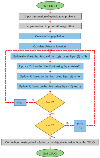
Figure 1.
Flowchart of “the good, the bad, and the ugly” optimizer (GBUO).
3. Simulation Study and Results
This section evaluates GBUO performance for optimization problem resolution. For this purpose, the proposed optimizer is implemented on a set of twenty-three standard objective functions.
3.1. Algorithms Used for Comparison and Objective Functions
The results of other well-known optimization algorithms are compared with those obtained by GBUO in order to further evaluate its capability for solving optimization problems. These optimization algorithms are genetic algorithm (GA), particle swarm optimization (PSO), gravitational search algorithm (GSA), teaching-learning-based optimization (TLBO), grey wolf optimizer (GWO), grasshopper optimization algorithm (GOA), spotted hyena optimizer (SHO), and marine predators algorithm (MPA). The values used for the main controlling parameters of the comparative algorithms are specified in Table 2.
Table 2.
Parameter values for the comparative algorithms.
The proposed optimizer’s performance and the eight optimization algorithms are evaluated for optimizing twenty-three different objective functions. These objective functions are classified into three types including unimodal, multimodal, and fixed-dimension multimodal functions. Information on these objective functions is provided in Appendix A, Table A1, Table A2 and Table A3.
The simulation and the algorithms have been implemented in the Matlab R2020a version, run in Microsoft Windows 10 with 64 bits on a Core i-7 processor with 2.40 GHz and 6GB memory. The average (Ave) and standard deviation (std) of the best obtained optimal solution until the last iteration are computed as performance evaluation metrics. Optimization algorithms utilize 20 independent runs for each objective function, where each run employs 1000 iterations to generate and report the results.
3.2. Results
In this section, simulation and implementation of optimization algorithms on standard objective functions are presented. A set of seven objective functions F1 to F7 is introduced as unimodal objective functions. Six objective functions F8 to F13 are considered multimodal objective functions. Finally, a set of ten objective functions F14 to F23 is introduced as fixed-dimension multimodal objective functions.
The optimization of the unimodal objective functions using GBUO and the mentioned eight optimization algorithms are presented in Table 3. According to the results in this table, GBUO and SHO are the best optimizers for F1 to F4 functions. After these two algorithms, TLBO is the third best optimizer for F1 to F4 functions. GBUO is also the best optimizer for F5 to F7 functions. Moreover, Table 4 presents the results for implementing the proposed optimizer compared with the eight optimization algorithms considered in this study for multimodal objective functions. According to this table, GBUO, SHO, MPA are the best optimizers for F9 and F11 objective functions. GBUO in F10 function has the best performance among algorithms. After the proposed algorithm, GWO is the second and SHO is the third best optimizers for F10. GA for F8, TLBO for F12, and GSA for F13 are the best optimizers. GBUO is the second-best optimizer on F8, F12, and F13. The results of applying the proposed optimizer and the eight other optimization algorithms on the third type objective functions are presented in Table 5. Based on the results in this table, GBUO provides the best performance in all F14 to F23 objective functions.
Table 3.
Results of applying optimization algorithms on unimodal objective functions.
Table 4.
Results of applying optimization algorithms on multimodal objective functions.
Table 5.
Results of applying optimization algorithms on fixed-dimension multimodal objective functions.
3.3. Statistical Testing
The optimization of standard test functions was presented as the average and standard deviation of the best solutions. However, these results alone are not enough to guarantee the superiority of the proposed algorithm. Even after twenty independent performances, this superiority may occur by chance despite its low probability. Therefore, the Friedman rank test is used to statistically evaluate the algorithms and further analyze the optimization results. The Friedman rank test is a non-parametric statistical test developed by Milton Friedman. Nonparametric means the test does not assume data comes from a particular distribution. The procedure involves ranking each row (or block) together, then considering the values of ranks by columns [90]. The steps for implementing the Friedman rank test are as follows:
Start.
Step1: Determine the results of different groups.
Step2: Rank each row of results based on the best result (here from 1 to 9).
Step3: Calculate the sum of the ranks of each column for different algorithms.
Step4: Determine the strongest algorithm to the weakest algorithm based on the sum of the ranks of each column.
End.
The Friedman rank test results for all three different objective functions: unimodal, multimodal, and fixed-dimension multimodal objective functions are presented in Table 6. Based on the results presented, for all three types of objective functions, the proposed GBUO has the first rank compared to other optimization algorithms. The overall results on all the objective functions (F1–F23) show that GBUO is significantly superior to other algorithms.
Table 6.
Results of the Friedman rank test for evaluate the optimization algorithms.
4. Discussion
Optimization algorithms based on random scanning of the search space have been widely used by researchers for solving optimization problems. Exploitation and exploration capabilities are two important indicators in the analysis of optimization algorithms. The exploitation capacity of an optimization algorithm means the ability of that algorithm to achieve and provide a quasi-optimal solution. Therefore, when comparing several optimization algorithms’ performance, an algorithm that provides a more appropriate quasi-optimal solution (closer to global optimal) has a higher exploitation capacity than other algorithms. An optimization algorithm’s exploration capacity means that the algorithm’s ability to accurately scan the search space, solving optimization problems with several local optimal solutions; the exploration capacity has a considerable effect on providing a quasi-optimal solution. In such problems, if the algorithm does not have the appropriate exploration capability, it provides non-optimal solutions by getting stuck in optimal local locals.
The unimodal objective functions F1 to F7 are functions that have only one global optimal solution and lack local optimal local. Therefore, this set of objective functions is suitable for analyzing the exploitation capacity of the optimization algorithms. Table 3 presents the results obtained from implementing the proposed GBUO and eight other optimization algorithms on the unimodal objective functions in order to properly evaluate the exploitation capacity. Evaluation of the results shows that the proposed optimizer provides more suitable quasi-optimal solutions than the other eight algorithms for all F1 to F7 objective functions. Accordingly, GBUO has a high exploitation capacity and is much more competitive than the other mentioned algorithms.
The second (F8 to F13) and the third (F14 to F23) categories of the objective functions have several local optimal solutions besides optimal solutions. Therefore, these types of objective functions are suitable for analyzing the exploration capability of the optimization algorithms. Table 4 and Table 5 present the results of implementing the proposed GBUO and eight other optimization algorithms on the multimodal objective functions to tolerate capability. The results presented in these tables show that the proposed GBUO has a good exploration capability. Moreover, the proposed GBUO can also find local-optimal solutions by accurately scanning the search space and thus, does not get stuck in local optimal to the other eight algorithms. The performance of the proposed GBUO is more appropriate and competitive for solving this type of optimization problem. It is confirmed that GBUO is a useful optimizer for solving different types of optimization problems.
5. Conclusions
In this paper, a new optimization method called “the good, the bad, and the ugly” optimizer (GBUO) has been introduced based on the effect of three members of the population on population updating. These three influential members include the good member with the best value of the objective function, the bad member with the worst value of the objective function, and the ugly member selected randomly. In GBUO, the population is updated in three phases; in the first phase, the population moves towards the good member, in the second phase, the population moves away from the bad member, and in the third phase, the population is updated on the ugly member. In a challenging move, the ugly member leads the population to situations contrary to society’s movement.
GBUO has been mathematically modeled and then implemented on a set of twenty-three different objective functions. In order to analyze the performance of the proposed optimizer in solving optimization problems, eight well-known optimization algorithms, including genetic algorithm (GA), particle swarm optimization (PSO), gravitational search algorithm (GSA), teaching-learning-based optimization (TLBO), grey wolf optimizer (GWO), whale optimization algorithm (WOA), spotted hyena optimizer (SHO), and marine predators algorithm (MPA) were considered for comparison.
The results demonstrated that the proposed optimizer has desirable and adequate performance for solving different optimization problems and is much more competitive than other mentioned algorithms.
The authors suggest some ideas and perspectives for future studies. For example, a multi-objective version of the GBUO is an exciting potential for this study. Some real-world optimization problems could be some significant contributions, as well.
Author Contributions
Conceptualization, M.D., Z.M. and H.G.; methodology, H.G.; software, Z.M. and M.D.; validation, R.A.R.-M. and N.N.; formal analysis, N.N., R.A.R.-M. and R.M.-M.; investigation, R.A.R.-M.; resources, Z.M. and M.D.; data curation, R.A.R.-M. and R.M.-M.; writing—original draft preparation, H.G., M.D., Z.M. and N.N.; writing—review and editing, R.A.R.-M. and R.M.-M.; supervision, M.D.; project administration, H.G.; funding acquisition, R.A.R.-M. and R.M.-M. All authors have read and agreed to the published version of the manuscript.
Funding
The current project was funded by Tecnologico de Monterrey and FEMSA Foundation (grant CAMPUSCITY project).
Institutional Review Board Statement
Not applicable.
Informed Consent Statement
Informed consent was obtained from all subjects involved in the study.
Data Availability Statement
The authors declare to honor the Principles of Transparency and Best Practice in Scholarly Publishing about Data.
Conflicts of Interest
The authors declare no conflict of interest.
Appendix A
Table A1.
Unimodal test functions.
Table A1.
Unimodal test functions.
Table A2.
Multimodal test functions
Table A2.
Multimodal test functions
Table A3.
Multimodal test functions with fixed dimension
Table A3.
Multimodal test functions with fixed dimension
| [−5,10] [0,15] | |
References
- Dehghani, M.; Montazeri, Z.; Malik, O.P. Energy commitment: A planning of energy carrier based on energy consumption. Electr. Eng. Electromech. 2019, 69–72. [Google Scholar] [CrossRef]
- Dehghani, M.; Mardaneh, M.; Malik, O.P.; Guerrero, J.M.; Sotelo, C.; Sotelo, D.; Nazari-Heris, M.; Al-Haddad, K.; Ramirez-Mendoza, R.A. Genetic Algorithm for Energy Commitment in a Power System Supplied by Multiple Energy Carriers. Sustainability 2020, 12, 53. [Google Scholar] [CrossRef]
- Ehsanifar, A.; Dehghani, M.; Allahbakhshi, M. Calculating the leakage inductance for transformer inter-turn fault detection using finite element method. In Proceedings of the 2017 Iranian Conference on Electrical Engineering (ICEE), Tehran, Iran, 2–4 May 2017; pp. 1372–1377. [Google Scholar]
- Dehghani, M.; Mardaneh, M.; Malik, O.P.; Guerrero, J.M.; Morales-Menendez, R.; Ramirez-Mendoza, R.A.; Matas, J.; Abusorrah, A. Energy Commitment for a Power System Supplied by Multiple Energy Carriers System using Following Optimization Algorithm. Appl. Sci. 2020, 10, 5862. [Google Scholar] [CrossRef]
- Dehghani, M.; Montazeri, Z.; Malik, O. Optimal sizing and placement of capacitor banks and distributed generation in distribution systems using spring search algorithm. Int. J. Emerg. Electr. Power Syst. 2020, 21. [Google Scholar] [CrossRef]
- Dehghani, M.; Montazeri, Z.; Malik, O.P.; Al-Haddad, K.; Guerrero, J.M.; Dhiman, G. A New Methodology Called Dice Game Optimizer for Capacitor Placement in Distribution Systems. Electr. Eng. Electromech. 2020, 61–64. [Google Scholar] [CrossRef]
- Dehbozorgi, S.; Ehsanifar, A.; Montazeri, Z.; Dehghani, M.; Seifi, A. Line loss reduction and voltage profile improvement in radial distribution networks using battery energy storage system. In Proceedings of the 2017 IEEE 4th International Conference on Knowledge-Based Engineering and Innovation (KBEI), Tehran, Iran, 22 December 2017; pp. 215–219. [Google Scholar]
- Montazeri, Z.; Niknam, T. Optimal utilization of electrical energy from power plants based on final energy consumption using gravitational search algorithm. Electr. Eng. Electromech. 2018, 70–73. [Google Scholar] [CrossRef]
- Dehghani, M.; Mardaneh, M.; Montazeri, Z.; Ehsanifar, A.; Ebadi, M.J.; Grechko, O.M. Spring search algorithm for simultaneous placement of distributed generation and capacitors. Electr. Eng. Electromech. 2018, 68–73. [Google Scholar] [CrossRef]
- Dehghani, M.; Montazeri, Z.; Ehsanifar, A.; Seifi, A.R.; Ebadi, M.J.; Grechko, O.M. Planning of energy carriers based on final energy consumption using dynamic programming and particle swarm optimization. Electr. Eng. Electromech. 2018, 62–71. [Google Scholar] [CrossRef]
- Montazeri, Z.; Niknam, T. Energy carriers management based on energy consumption. In Proceedings of the 2017 IEEE 4th International Conference on Knowledge-Based Engineering and Innovation (KBEI), Tehran, Iran, 22 December 2017; pp. 539–543. [Google Scholar]
- Aarts, E.; Korst, J. Simulated Annealing and Boltzmann Machines: A Stochastic Approach to Combinatorial Optimization and Neural Computing; John Wiley & Sons, Inc.: New York, NY, USA, 1988. [Google Scholar]
- Dehghani, M.; Montazeri, Z.; Dhiman, G.; Malik, O.; Morales-Menendez, R.; Ramirez-Mendoza, R.A.; Dehghani, A.; Guerrero, J.M.; Parra-Arroyo, L. A spring search algorithm applied to engineering optimization problems. Appl. Sci. 2020, 10, 6173. [Google Scholar] [CrossRef]
- Dehghani, M.; Montazeri, Z.; Dehghani, A.; Nouri, N.; Seifi, A. BSSA: Binary spring search algorithm. In Proceedings of the 2017 IEEE 4th International Conference on Knowledge-Based Engineering and Innovation (KBEI), Tehran, Iran, 22 December 2017; pp. 220–224. [Google Scholar]
- Dorigo, M.; Birattari, M.; Stutzle, T. Ant colony optimization. IEEE Comput. Intell. Mag. 2006, 1, 28–39. [Google Scholar] [CrossRef]
- Givi, H.; Noroozi, M.A.; Vahidi, B.; Moghani, J.S.; Zand, M.A.V. A Novel Approach for Optimization of Z-Matrix Building Process Using Ant Colony Algorithm. J. Basic Appl. Sci. Res. 2012, 2, 8932–8937. [Google Scholar]
- Kennedy, J.; Eberhart, R. Particle swarm optimization. In Proceedings of the ICNN′95—International Conference on Neural Networks, Perth, WA, Australia, 27 November–1 December 1995; pp. 1942–1948. [Google Scholar]
- Gandomi, A.H.; Yang, X.-S.; Alavi, A.H. Cuckoo search algorithm: A metaheuristic approach to solve structural optimization problems. Eng. Comput. 2013, 29, 17–35. [Google Scholar] [CrossRef]
- Eberhart, R.C.; Shi, Y.; Kennedy, J. Swarm Intelligence; Elsevier: Amsterdam, The Netherlands, 2001. [Google Scholar]
- Kirkpatrick, S.; Gelatt, C.D.; Vecchi, M.P. Optimization by simulated annealing. Science 1983, 220, 671–680. [Google Scholar] [CrossRef]
- Faramarzi, A.; Afshar, M. Application of cellular automata to size and topology optimization of truss structures. Sci. Iran. 2012, 19, 373–380. [Google Scholar] [CrossRef]
- Dehghani, M.; Montazeri, Z.; Dehghani, A.; Malik, O.P.; Morales-Menendez, R.; Dhiman, G.; Nouri, N.; Ehsanifar, A.; Guerrero, J.M.; Ramirez-Mendoza, R.A. Binary Spring Search Algorithm for Solving Various Optimization Problems. Appl. Sci. 2021, 11, 1286. [Google Scholar] [CrossRef]
- Dehghani, M.; Montazeri, Z.; Dehghani, A.; Samet, H.; Sotelo, C.; Sotelo, D.; Ehsanifar, A.; Malik, O.P.; Guerrero, J.M.; Dhiman, G. DM: Dehghani Method for Modifying Optimization Algorithms. Appl. Sci. 2020, 10, 7683. [Google Scholar] [CrossRef]
- Yang, X.-S.; Deb, S. Cuckoo search via Lévy flights. In Proceedings of the 2009 World Congress on Nature & Biologically Inspired Computing (NaBIC); IEEE: Piscataway, NJ, USA, 2009; pp. 210–214. [Google Scholar]
- Yazdani, M.; Jolai, F. Lion optimization algorithm (LOA): A nature-inspired metaheuristic algorithm. J. Comput. Des. Eng. 2016, 3, 24–36. [Google Scholar] [CrossRef]
- Saremi, S.; Mirjalili, S.; Lewis, A. Grasshopper optimisation algorithm: Theory and application. Adv. Eng. Softw. 2017, 105, 30–47. [Google Scholar] [CrossRef]
- Dhiman, G.; Kumar, V. Emperor penguin optimizer: A bio-inspired algorithm for engineering problems. Knowl. Based Syst. 2018, 159, 20–50. [Google Scholar] [CrossRef]
- Kallioras, N.A.; Lagaros, N.D.; Avtzis, D.N. Pity beetle algorithm—A new metaheuristic inspired by the behavior of bark beetles. Adv. Eng. Softw. 2018, 121, 147–166. [Google Scholar] [CrossRef]
- Jahani, E.; Chizari, M. Tackling global optimization problems with a novel algorithm—Mouth Brooding Fish algorithm. Appl. Soft Comput. 2018, 62, 987–1002. [Google Scholar] [CrossRef]
- Shadravan, S.; Naji, H.; Bardsiri, V.K. The Sailfish Optimizer: A novel nature-inspired metaheuristic algorithm for solving constrained engineering optimization problems. Eng. Appl. Artif. Intell. 2019, 80, 20–34. [Google Scholar] [CrossRef]
- Dehghani, M.; Mardaneh, M.; Malik, O. FOA: “Following“Optimization Algorithm for solving Power engineering optimization problems. J. Oper. Autom. Power Eng. 2020, 8, 57–64. [Google Scholar]
- Dehghani, M.; Montazeri, Z.; Dehghani, A.; Mendoza, R.R.; Samet, H.; Guerrero, J.M.; Dhiman, G. MLO: Multi Leader Optimizer. Int. J. Intell. Eng. Syst. 2020. [Google Scholar] [CrossRef]
- Holland, J.H. Genetic algorithms. Sci. Am. 1992, 267, 66–73. [Google Scholar] [CrossRef]
- Storn, R.; Price, K. Differential evolution–a simple and efficient heuristic for global optimization over continuous spaces. J. Glob. Optim. 1997, 11, 341–359. [Google Scholar] [CrossRef]
- Banzhaf, W.; Nordin, P.; Keller, R.E.; Francone, F.D. Genetic Programming; Springer: Berlin/Heidelberg, Germany, 1998. [Google Scholar]
- Beyer, H.-G.; Schwefel, H.-P. Evolution strategies–A comprehensive introduction. Nat. Comput. 2002, 1, 3–52. [Google Scholar] [CrossRef]
- Simon, D. Biogeography-based optimization. IEEE Trans. Evol. Comput. 2008, 12, 702–713. [Google Scholar] [CrossRef]
- Huang, G. Artificial infectious disease optimization: A SEIQR epidemic dynamic model-based function optimization algorithm. Swarm Evol. Comput. 2016, 27, 31–67. [Google Scholar] [CrossRef]
- Labbi, Y.; Attous, D.B.; Gabbar, H.A.; Mahdad, B.; Zidan, A. A new rooted tree optimization algorithm for economic dispatch with valve-point effect. Int. J. Electr. Power Energy Syst. 2016, 79, 298–311. [Google Scholar] [CrossRef]
- Baykasoğlu, A.; Akpinar, Ş. Weighted Superposition Attraction (WSA): A swarm intelligence algorithm for optimization problems–Part 1: Unconstrained optimization. Appl. Soft Comput. 2017, 56, 520–540. [Google Scholar] [CrossRef]
- Akyol, S.; Alatas, B. Plant intelligence based metaheuristic optimization algorithms. Artif. Intell. Rev. 2017, 47, 417–462. [Google Scholar] [CrossRef]
- Salmani, M.H.; Eshghi, K. A metaheuristic algorithm based on chemotherapy science: CSA. J. Optim. 2017, 2017, 3082024. [Google Scholar] [CrossRef]
- Cheraghalipour, A.; Hajiaghaei-Keshteli, M.; Paydar, M.M. Tree Growth Algorithm (TGA): A novel approach for solving optimization problems. Eng. Appl. Artif. Intell. 2018, 72, 393–414. [Google Scholar] [CrossRef]
- Kirkpatrick, S.; Gelatt, C.D.; Vecchi, M.P. A heuristic algorithm and simulation approach to relative location of facilities. Optim. Simulated Annealing 1983, 220, 671–680. [Google Scholar]
- Banerjee, K. Generalized Inverse of Matrices and Its Applications; Taylor & Francis Group: Abingdon, UK, 1973. [Google Scholar]
- Eskandar, H.; Sadollah, A.; Bahreininejad, A.; Hamdi, M. Water cycle algorithm–A novel metaheuristic optimization method for solving constrained engineering optimization problems. Comput. Struct. 2012, 110, 151–166. [Google Scholar] [CrossRef]
- Kaveh, A.; Bakhshpoori, T. Water evaporation optimization: A novel physically inspired optimization algorithm. Comput. Struct. 2016, 167, 69–85. [Google Scholar] [CrossRef]
- Muthiah-Nakarajan, V.; Noel, M.M. Galactic Swarm Optimization: A new global optimization metaheuristic inspired by galactic motion. Appl. Soft Comput. 2016, 38, 771–787. [Google Scholar] [CrossRef]
- Dehghani, M.; Montazeri, Z.; Dehghani, A.; Seifi, A. Spring search algorithm: A new meta-heuristic optimization algorithm inspired by Hooke′s law. In Proceedings of the 2017 IEEE 4th International Conference on Knowledge-Based Engineering and Innovation (KBEI), Tehran, Iran, 22 December 2017; pp. 210–214. [Google Scholar]
- Zhang, Q.; Wang, R.; Yang, J.; Ding, K.; Li, Y.; Hu, J. Collective decision optimization algorithm: A new heuristic optimization method. Neurocomputing 2017, 221, 123–137. [Google Scholar] [CrossRef]
- Vommi, V.B.; Vemula, R. A very optimistic method of minimization (VOMMI) for unconstrained problems. Inf. Sci. 2018, 454, 255–274. [Google Scholar] [CrossRef]
- Dehghani, M.; Samet, H. Momentum search algorithm: A new meta-heuristic optimization algorithm inspired by momentum conservation law. SN Appl. Sci. 2020, 2, 1–15. [Google Scholar] [CrossRef]
- Dehghani, M.; Montazeri, Z.; Malik, O.P. DGO: Dice Game Optimizer. Gazi Univ. J. Sci. 2019, 32. [Google Scholar] [CrossRef]
- Dehghani, M.; Montazeri, Z.; Malik, O.P.; Ehsanifar, A.; Dehghani, A. OSA: Orientation search algorithm. Int. J. Ind. Electron. Control Optim. 2019, 2, 99–112. [Google Scholar]
- Dehghani, M.; Montazeri, Z.; Saremi, S.; Dehghani, A.; Malik, O.P.; Al-Haddad, K.; Guerrero, J.M. HOGO: Hide Objects Game Optimization. Int. J. Intell. Eng. Syst. 2020, 13, 216–225. [Google Scholar]
- Dehghani, M.; Mardaneh, M.; Guerrero, J.M.; Malik, O.; Kumar, V. Football game based optimization: An application to solve energy commitment problem. Int. J. Intell. Eng. Syst. 2020, 13, 514–523. [Google Scholar] [CrossRef]
- Dehghani, M.; Montazeri, Z.; Givi, H.; Guerrero, J.M.; Dhiman, G. Darts game optimizer: A new optimization technique based on darts game. Int. J. Intell. Eng. Syst. 2020, 13, 286–294. [Google Scholar] [CrossRef]
- Dehghani, M.; Montazeri, Z.; Malik, O.P.; Givi, H.; Guerrero, J.M. Shell game optimization: A novel game-based algorithm. Int. J. Intell. Eng. Syst. 2020, 13, 246–255. [Google Scholar]
- Gao, K.Z.; Suganthan, P.N.; Chua, T.J.; Chong, C.S.; Cai, T.X.; Pan, Q.K. A two-stage artificial bee colony algorithm scheduling flexible job-shop scheduling problem with new job insertion. Expert Syst. Appl. 2015, 42, 7652–7663. [Google Scholar] [CrossRef]
- Wang, H.; Guo, F.; Yao, H.; He, S.; Xu, X. Collision avoidance planning method of USV based on improved ant colony optimization algorithm. IEEE Access 2019, 7, 52964–52975. [Google Scholar] [CrossRef]
- Wang, L.; Zhong, Y.; Yin, Y. Nearest neighbour cuckoo search algorithm with probabilistic mutation. Appl. Soft Comput. 2016, 49, 498–509. [Google Scholar] [CrossRef]
- Pan, W.-T. A new fruit fly optimization algorithm: Taking the financial distress model as an example. Knowl. Based Syst. 2012, 26, 69–74. [Google Scholar] [CrossRef]
- Yang, X.-S. Firefly algorithm, stochastic test functions and design optimisation. Int. J. Bio Inspired Comput. 2010, 2, 78–84. [Google Scholar] [CrossRef]
- Mirjalili, S.; Mirjalili, S.M.; Lewis, A. Grey wolf optimizer. Adv. Eng. Softw. 2014, 69, 46–61. [Google Scholar] [CrossRef]
- Dehghani, M.; Mardaneh, M.; Guerrero, J.M.; Malik, O.P.; Ramirez-Mendoza, R.A.; Matas, J.; Vasquez, J.C.; Parra-Arroyo, L. A new “Doctor and Patient” optimization algorithm: An application to energy commitment problem. Appl. Sci. 2020, 10, 5791. [Google Scholar] [CrossRef]
- Dehghani, M.; Mardaneh, M.; Malik, O.P.; NouraeiPour, S.M. DTO: Donkey theorem optimization. In Proceedings of the 2019 27th Iranian Conference on Electrical Engineering (ICEE), Yazd, Iran, 30 April–2 May 2019; pp. 1855–1859. [Google Scholar]
- Dehghani, M.; Montazeri, Z.; Dehghani, A.; Malik, O.P. GO: Group optimization. Gazi Univ. J. Sci. 2020, 33, 381–392. [Google Scholar] [CrossRef]
- Jain, M.; Singh, V.; Rani, A. A novel nature-inspired algorithm for optimization: Squirrel search algorithm. Swarm Evol. Comput. 2019, 44, 148–175. [Google Scholar] [CrossRef]
- Zhang, X.; Zhao, K.; Wang, L.; Wang, Y.; Niu, Y. An Improved Squirrel Search Algorithm with Reproductive Behavior. IEEE Access 2020. [Google Scholar] [CrossRef]
- Mirjalili, S. Dragonfly algorithm: A new meta-heuristic optimization technique for solving single-objective, discrete, and multi-objective problems. Neural Comput. Appl. 2016, 27, 1053–1073. [Google Scholar] [CrossRef]
- Meng, Z.; Pan, J.-S.; Xu, H. QUasi-Affine TRansformation Evolutionary (QUATRE) algorithm: A cooperative swarm based algorithm for global optimization. Knowl.Based Syst. 2016, 109, 104–121. [Google Scholar] [CrossRef]
- Li, S.; Chen, H.; Wang, M.; Heidari, A.A.; Mirjalili, S. Slime mould algorithm: A new method for stochastic optimization. Future Gener. Comput. Syst. 2020. [Google Scholar] [CrossRef]
- Faramarzi, A.; Heidarinejad, M.; Stephens, B.; Mirjalili, S. Equilibrium optimizer: A novel optimization algorithm. Knowl. Based Syst. 2020, 191, 105190. [Google Scholar] [CrossRef]
- Hashim, F.A.; Houssein, E.H.; Mabrouk, M.S.; Al-Atabany, W.; Mirjalili, S. Henry gas solubility optimization: A novel physics-based algorithm. Future Gener. Comput. Syst. 2019, 101, 646–667. [Google Scholar] [CrossRef]
- Pan, J.-S.; Meng, Z.; Xu, H.; Li, X. QUasi-Affine TRansformation Evolution (QUATRE) algorithm: A new simple and accurate structure for global optimization. In Proceedings of the International Conference on Industrial, Engineering and Other Applications of Applied Intelligent Systems; Springer: Berlin/Heidelberg, Germany, 2016; pp. 657–667. [Google Scholar]
- Meng, Z.; Pan, J.-S. QUasi-Affine TRansformation Evolution with External ARchive (QUATRE-EAR): An enhanced structure for differential evolution. Knowl. Based Syst. 2018, 155, 35–53. [Google Scholar] [CrossRef]
- Wolpert, D.H.; Macready, W.G. No free lunch theorems for optimization. IEEE Trans. Evol. Comput. 1997, 1, 67–82. [Google Scholar] [CrossRef]
- Heidari, A.A.; Mirjalili, S.; Faris, H.; Aljarah, I.; Mafarja, M.; Chen, H. Harris hawks optimization: Algorithm and applications. Future Gener. Comput. Syst. 2019, 97, 849–872. [Google Scholar] [CrossRef]
- Yıldız, A.R.; Yıldız, B.S.; Sait, S.M.; Li, X. The Harris hawks, grasshopper and multi-verse optimization algorithms for the selection of optimal machining parameters in manufacturing operations. Mater. Test. 2019, 61, 725–733. [Google Scholar] [CrossRef]
- Jia, H.; Lang, C.; Oliva, D.; Song, W.; Peng, X. Dynamic harris hawks optimization with mutation mechanism for satellite image segmentation. Remote Sens. 2019, 11, 1421. [Google Scholar] [CrossRef]
- Chen, H.; Jiao, S.; Wang, M.; Heidari, A.A.; Zhao, X. Parameters identification of photovoltaic cells and modules using diversification-enriched Harris hawks optimization with chaotic drifts. J. Clean. Prod. 2020, 244, 118778. [Google Scholar] [CrossRef]
- Golilarz, N.A.; Gao, H.; Demirel, H. Satellite image de-noising with harris hawks meta heuristic optimization algorithm and improved adaptive generalized gaussian distribution threshold function. IEEE Access 2019, 7, 57459–57468. [Google Scholar] [CrossRef]
- Mehta, M.S.; Singh, M.B.; Gagandeep, M. Harris Hawks optimization for solving optimum load dispatch problem in power system. Int. J. Eng. Res. Technol. 2019, 8, 962–968. [Google Scholar]
- Houssein, E.H.; Saad, M.R.; Hussain, K.; Zhu, W.; Shaban, H.; Hassaballah, M. Optimal sink node placement in large scale wireless sensor networks based on Harris’ hawk optimization algorithm. IEEE Access 2020, 8, 19381–19397. [Google Scholar] [CrossRef]
- Hussain, K.; Zhu, W.; Salleh, M.N.M. Long-term memory Harris’ hawk optimization for high dimensional and optimal power flow problems. IEEE Access 2019, 7, 147596–147616. [Google Scholar] [CrossRef]
- Fan, Q.; Chen, Z.; Xia, Z. A novel quasi-reflected Harris hawks optimization algorithm for global optimization problems. Soft Comput. 2020, 1–19. [Google Scholar] [CrossRef]
- Kurtuluş, E.; Yıldız, A.R.; Sait, S.M.; Bureerat, S. A novel hybrid Harris hawks-simulated annealing algorithm and RBF-based metamodel for design optimization of highway guardrails. Mater. Test. 2020, 62, 251–260. [Google Scholar] [CrossRef]
- Moayedi, H.; Nguyen, H.; Rashid, A.S.A. Comparison of dragonfly algorithm and Harris hawks optimization evolutionary data mining techniques for the assessment of bearing capacity of footings over two-layer foundation soils. Eng. Comput. 2019, 1–11. [Google Scholar] [CrossRef]
- Kamboj, V.K.; Nandi, A.; Bhadoria, A.; Sehgal, S. An intensify Harris Hawks optimizer for numerical and engineering optimization problems. Appl. Soft Comput. 2020, 89, 106018. [Google Scholar] [CrossRef]
- Daniel, W.W. Friedman two-way analysis of variance by ranks. In Applied Nonparametric Statistics, 2nd ed.; PWS-Kent: Boston, MA, USA, 1990; pp. 262–274. [Google Scholar]
Publisher’s Note: MDPI stays neutral with regard to jurisdictional claims in published maps and institutional affiliations. |
© 2021 by the authors. Licensee MDPI, Basel, Switzerland. This article is an open access article distributed under the terms and conditions of the Creative Commons Attribution (CC BY) license (http://creativecommons.org/licenses/by/4.0/).