Thermal Strain-Based Simplified Prediction of Thermal Deformation Caused by Flame Bending

Abstract

This paper describes a quick and accurate method for predicting thermal deformation due to flame bending of the curved plate located before and after the hull. Flame bending is a common method to deform the curved plate used in shipyards. Three-dimensional thermo-elasto-plastic analysis is known as the most accurate method for predicting deformed shape in the automation of frame bending. However, the three-dimensional analysis takes a lot of computational time. The quick prediction method, strain as direct boundary (SDB), was introduced, which is a simplified prediction method based on thermal strain. This simplified method implements an equivalent load as a temperature difference that can simulate thermal deformation by flame. In the case of multiple heating lines by the flame bending, the residual strain generated by the first heating line affects the other lines. To consider the effect of residual strain, the plastic material properties are also considered. Then, the distance ratio from the center line is used to generate the same temperature field in grid mesh. The results of the prediction were evaluated for the heat affected zone (HAZ) of the specimen obtained through the flame bending experiment. Therefore, this paper introduced detail procedure of the proposed SDB method and the experimental results for the practical application.

1. Introduction

In the shipbuilding industry, flame bending is an economical method to form the complex curved hull plate located on the bow or stern of the ship. As intelligent manufacturing technology using information and communications technology (ICT) is being developed, the shipbuilding industry is also expanding its intelligent technology. These technologies are applied to various ship production processes, but the forming of curved plates of the hull is still difficult to automate. When multiple flame bending condition is applied, it is difficult to predict the strain according to the heating line. Therefore, a method for predicting the thermal deformation by the flaming bending should be developed in advance. To predict the thermal deformation of the steel plate by flame bending, a finite element method considering both heat transfer and thermal deformation has been proposed by many studies [1,2,3,4]. Nevertheless, predicting the thermal deformation by multi-heating lines is a difficult task. Although rezoning techniques have been adapted to reduce the computational time and the speed of the computer has also increased, it still takes several hours [5]. Therefore, the classical thermo-elasto-plastic analysis, which calculates the thermal deformation caused by the heat transfer by flame, is not suitable for a real-time prediction system.

In order to overcome these limitations, the equivalent load method based on the magnitude of inherent strain with shell elements was introduced by Jang et al. [6]. This method assumes that the area heated above the critical temperature is a heat-affected zone (HAZ) with residual deformation and performs elastic analysis by calculating the equivalent loads that can simulate the corresponding residual strain. When applying equivalent loads, it is complicated to define the rigidity or anisotropy of the plate. In addition, the definition of direction and magnitude of load for the automated strain analysis model is difficult because the heating line is replaced with a bending moment and shrinkage force as a boundary condition. Jang et al. [7] suggested an inherent strain-calculating method considering the phase transformation by flame. This method assumes that the plate has different material properties when it is heated and cooled. They considered that when the martensite volumetric expansion was generated, the tensile stress in the heated region, which affected the magnitude of the inherent strain in the cooling phase, was released. The strain as direct boundary (SDB) method, based on inherent strain, was introduced to overcome the disadvantages of the equivalent load method [6,7,8,9]. This method applies the inherent strain as the thermal expansion coefficient of a shell element, and the virtual temperature gradient, which can simulate the residual strain, is applied as the boundary condition, so equivalent thermal strain is naturally generated. The inherent strain region is bound by the transformation temperatures. The temperature is the lower transformation temperature, where austenite begins to form during heating of the steel.

This paper discusses both inherent strain and thermal strain-based approaches to predict the deformation of the shell forming by flame bending (or line heating). Taking into account the equivalent loads assumed from both inherent strain and thermal strain, deformation is predicted by the finite element analysis using shell elements. In addition, an elastic plastic finite element model based on the thermal strain is suggested by Ha [8]. In the flame bending process, multiple line heating is common. This suggested method made it possible to reflect the effects of the previous heating lines. The thermal strain can be given as a boundary condition by appropriately determining the heat-affected zone. In general, the sectional shape of the HAZ can be measured through welding experiments to determine the heat-affected zone [10]. Jang et al. [6] suggested that the HAZ can be determined from the phase transformation temperature. The HAZ of metallic materials depends on the temperature of the materials that undergo heat treatment. In other words, HAZ is determined by the phase transformation temperature.

In this paper, the SDB method was introduced based on thermal strain, which is most suitable among the several methods for predicting the residual thermal deformation of the hull plates by flame bending. In addition, the efficiency and accuracy of the SDB method were verified by comparing it with the experimental results for case studies of curved plates.

2. Prediction of Thermal Deformation

This section introduces the SDB method to simulate thermal deformations by flame bending. Firstly, the simulation process is described, which includes a method that reflects the material properties by considering the change in the state of the metal material with temperature. Then, the shape of the inherent strain zone and the virtual temperature profiles are discussed. The thermal expansion coefficient and the thermal strain calculation process considering the phase change are also explained. The SDB method consists of the above procedures and is described in detail as follows.

2.1. Residual Strain

In general, the residual strain can be considered as a source of deformations and residual stresses resulting from heat processes such as welding, cutting, heating, and bending. Thus, if the residual strain is known, the deformation and residual stress can be estimated using simplified analysis instead of 3D thermo-elasto-plastic analysis. In this way, the computation time can be greatly reduced. Therefore, in the SDB method, it is very important to determine the residual strain. The process of generating residual strain can be divided into two stages: a heating phase that undergoes heating and a cooling cycle that cools down from high temperature to room temperature. Here, it is assumed that the plastic stress and strain of the material do not occur when the material is tensile from heating but are caused by the shrinkage of the material during the cooling cycle [10]. Thus, the deformation of the plate mainly occurs during the cooling phase. The analysis is performed assuming that the thermal strain is the initial strain of the HAZ, and that the surrounding area is an element that constrains the HAZ. Equation (1) shows that the total strain (${\epsilon }^{total}$) through the process of flame bending (or line heating) is mainly divided into four parts: plastic strain (${\epsilon }^p$), elastic strain (${\epsilon }^e$), thermal strain (${\epsilon }^{th}$), and phase transformation strain (${\epsilon }^{ph}$).

$${\epsilon }^{total}={\epsilon }^p+{\epsilon }^e+{\epsilon }^{th}+{\epsilon }^{ph}$$

(1)

Since the deformation and the stress are produced by the total strain and elastic strain, residual strain in flame bending includes plastic, thermal, and phase transformation [8,9]. Considering that the distortion and the residual stress are produced by the residual strain, the inherent strain can be expressed by Equation (2) [6]. This relationship is shown in Figure 1.

The effect of the previous heating lines is so great that it is impossible to accurately predict the thermal deformation by elastic analysis based on improved inherent strain as shown in Figure 1. Therefore, the elastic-plastic analysis based on thermal strain is presented [8,10]. If the thermal strain (including phase transformation strain) replaces the improved inherent strain as the thermal expansion coefficient in the SDB method, it can reflect the plastic strain generated by previous heating lines. Thus, the elastic-plastic analysis based on thermal strain should be more accurate in multiple heating-line systems.

$${\epsilon }^{*}= {\epsilon }^{total}-{\epsilon }^e= {\epsilon }^p+{\epsilon }^{th}+{\epsilon }^{ph}$$

(2)

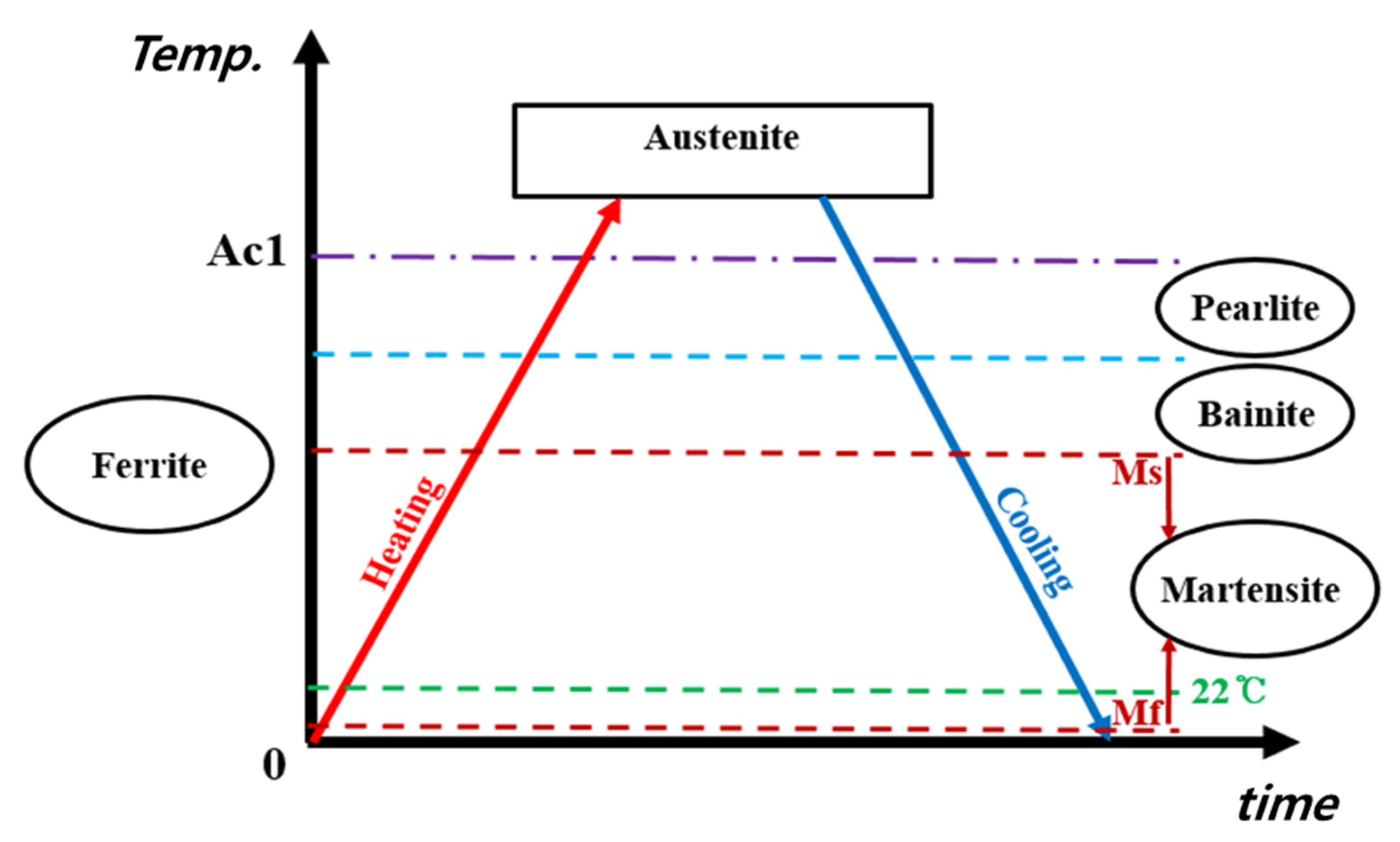
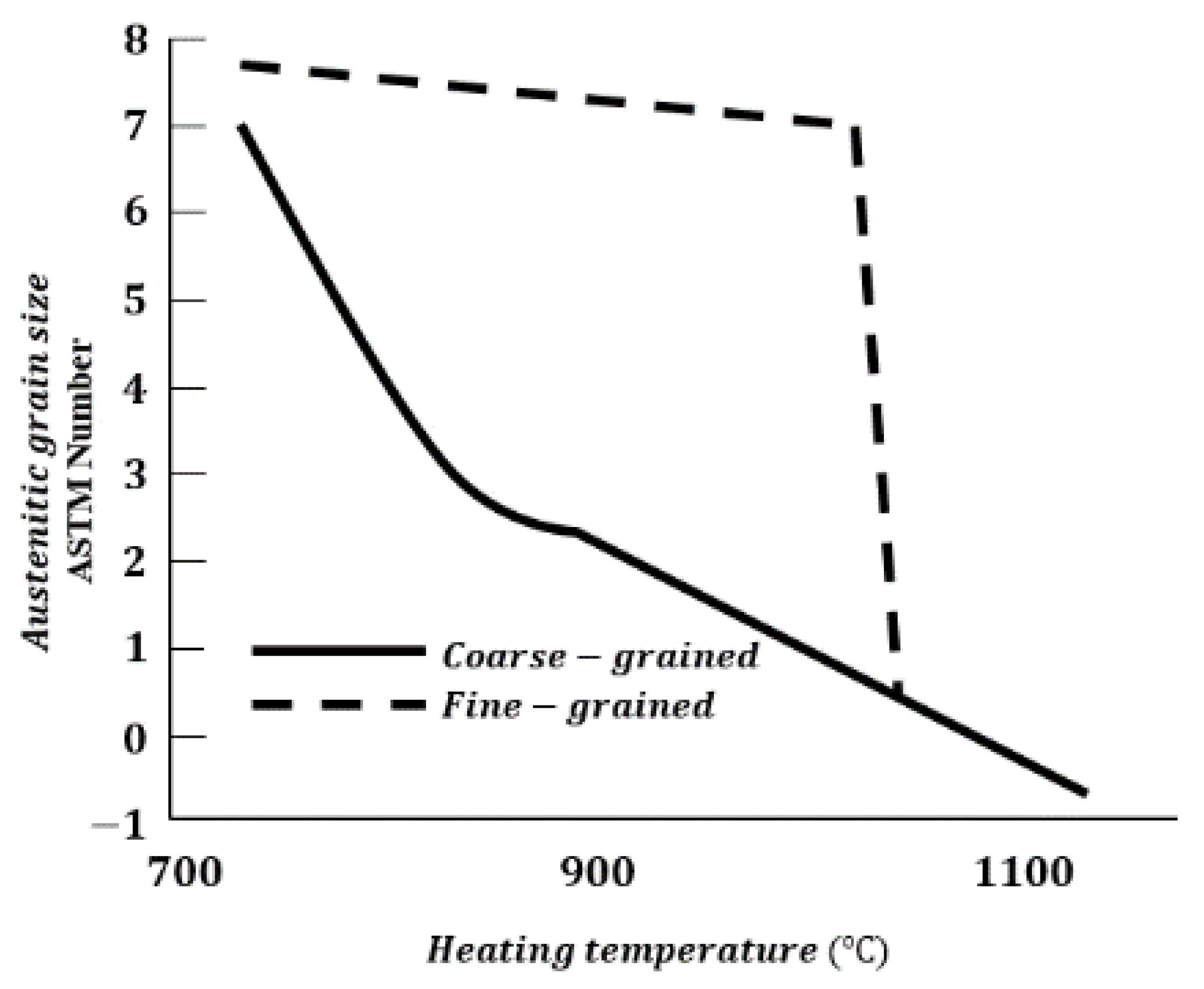
2.2. Phase Transformation during Heating and Cooling Cycle

During the flame bending process, the heated plate is subjected to rapid cooling so that the phase transformation of the metal crystal structure occurs [11]. In general, a hull plate of the mild A-grade steel formed by flame bending is converted into austenite by a heat source during the flame heating. The deformation caused by line heating occurs only on the surface of the austenite transformation, which begins with multiple phases due to the high temperature as shown in Figure 2. Thus, the austenite parts are all under the influence of water cooling. In such cases, a certain depth from the representation will result in a martensite transformation [9].

The $Ac1$ is the lower-phase transformation temperature at which austenite begins to form during heating of the steel as shown in Equation (3). It can be calculated by the function of the chemical composition of steel as described in

Table 1. Chemical composition of mild A-grade steel.

Grade A	C	Si	Mn	P	S
Wt%	0.18	0.45	0.02	0.02	0.02

. The $M_S$ temperature is the temperature at which martensite begins to form upon cooling [12]. When the steel is heated, and temperature reached $Ac1$, the ferrite is converted to austenite. As soon as the temperature passes the $M_S$, the remaining austenite starts being transformed into martensite. The temperature $M_S$ is a function of chemical composition in steel as shown in Equation (4) [13].

$$\mathrm{Ac}1=723-10.7\mathrm{Mn}-16.9\mathrm{Ni}+29.1\mathrm{Si}+16.9\mathrm{Cr}+290\mathrm{As}+6.38\mathrm{W}$$

(3)

$$\begin{gathered} Ms=512-453C-16.9Ni+15Cr-9.5Mo+217{\left(C\right)}^2 \\ -71.5\left(C\right)\left(Mn\right)-67.6\left(C\right)\left(Cr\right)-11.1Si \end{gathered}$$

(4)

Using the phase-starting temperature of each phase, the portion of austenite (γ) and martensite ($M$), depending on the temperature, can be calculated during the cooling cycle [11].

In this paper, it is assumed that the heated area above the critical temperature is converted to austenite during the heating phase [14]. The phase transformation not only changes the thermal expansion coefficient, elastic modulus, and fraction of microstructure, but also changes the magnitude of the inherent strain. The temperature $M_f$ at which the martensitic transformation finishes is lower than room temperature. When the temperature falls to room temperature, the mild steel has various crystal structures, such as residual austenite, martensite, ferrite, and pearlite. If the austenite is almost transformed into martensite, the volume fraction of martensite at temperature $T$ can be represented by Koistinen and Marburger [14]. Therefore, it is also assumed that all austenite transforms into martensite during the cooling process because the temperature $M_f$, at which martensite transformation stops, is lower than room temperature. During the cooling phase, the portion of austenite ($X_{\gamma }$) and martensite ($X_M$) according to each temperature can be expressed as Equations (5) and (6) [14].

$$X_{\gamma }\left(T\right)=e^{k·max\left[\left(M_s-T\right),0\right]}$$

(5)

$$X_M\left(T\right)=1-X_{\gamma }\left(T\right)=1-e^{k·max\left[\left(M_s-T\right),0\right]}$$

(6)

where $k$ is a phase transformation velocity constant depending on the material. If the austenite is transformed into martensite as a carbon steel (0.2 wt.%C), the value of $k$ is −0.026 [15]. Once the portion of retained austenite is measured using X-ray diffraction, $k$ can be updated using the experimental data.

2.3. Material Properties during Cooling Phase

Predicting thermal deformation requires the material properties of each cycle formed in the heating and cooling process, which can be expressed as a function of temperature, reflecting changes in the material phase according to the thermal analysis procedure. The material properties in the cooling case are defined by Equations (7)–(9) [9,16].

$${\alpha }_C\left(T\right)=\left(8e^{k·max\left[\left(M_s-T\right),0\right]}+13\right)\times {10}^{-6}$$

(7)

$$E_C\left(T\right)=\left(-3.333T{e}^{kmax\left[Ms-T,0\right]}-5T+20000\right)\times 0.98$$

(8)

$${\nu }_C\left(T\right)=-0.2e^{-0.001824T}+0.5$$

(9)

where ${\nu }_C$, $E_C$ ($Kgf/m{m}^2)$, ${\alpha }_C$denote Poisson’s ratio, Young’s modulus, and the thermal expansion coefficient in the cooling cycle, respectively. In the cooling cycle, the yield stress (${\sigma }_{YC}$) of martensite is larger than that of ferrite because martensite volumetric expansion can relax the tensile stress in the heated region [16]. Therefore, according to the maximum temperature of austenite, the austenite grain size ASTM (American Society of Mechanical Engineers) number and diameter of the average grain of the mild A-grade steel can be obtained from Figure 3 using Equations (10) and (11) [17].

$$ASTM=-\frac{T_C+T_{max}}{1000}+9.2$$

(10)

$$AGS\left(D\right)=0.359e^{-0.3464ASTM}$$

(11)

where $T_C$ is the critical temperature which is equal to $Ac1$ (Equation (3)), $T_{max}$is the maximum temperature in the whole process and $AGS$ is the average grain size $D$.

Hence, the yield stress in cooling can be obtained by Equation (12) [18,19], assuming that the grain is 100% fine-grained. Due to the different temperature in HAZ, the yield stress in cooling is not regarded as a value but as a range [20]. Therefore, the average maximum temperature and critical temperature should be used in Equation (10).

$${\sigma }_{YC}=\left(370+\frac{27.1}{\sqrt{D}}\right)+\left(480-370\right)\frac{\sqrt{C}}{\sqrt{0.2}}+\frac{\sqrt{C}}{\sqrt{0.2}}·\frac{48.0-27.1}{\sqrt{D}}$$

(12)

where $D$ is the average grain size and $C$ is the content of carbon in steel, as described in Table 1.

2.4. Modified Thermal Strain

During the cooling phase, volume expansion occurs due to phase transformation while austenite is transformed into martensite. The volumetric expansion ratio after heating and cooling in carbon steel can be calculated by Equation (13) [21].

$$\frac{\Delta V}{V}(\%)=X_M\left(T\right)\frac{\left(2.86+0.117C\right)·{\left(2.86-0.0143C\right)}^2}{{2.86}^3}+X_{F-P}-1$$

(13)

where $X_{F-P}$ represents the portion of ferrite and pearlite.

In this paper, it is assumed that only austenite or martensite exist in HAZ, so $X_{F-P}$ is zero. In the cooling cycle, the thermal strain can be calculated by the integral of the thermal expansion coefficient expressed in Equation (14), and the phase transformation strain is caused by the volumetric expansion of the phase transformation. Therefore, the sum of thermal strain and phase transformation strain, called modified thermal strain, is represented by Equation (15). Taking the derivative of Equation (15) gives the equivalent thermal expansion coefficient of the cooling cycle ${\alpha }_C^m\left(T\right)$, which can reflect both the linear thermal expansion and the volumetric expansion due to the phase transformation defined by Equation (16). Therefore, the modified thermal expansion coefficient is obtained from the derivative of modified thermal strain with respect to temperature, as shown in Figure 4.

$${\epsilon }_C^{th}\left(T\right)={\alpha }_C\left(T\right)·\Delta T={\int }_0^T{\alpha }_C\left(T\right)dT$$

(14)

$${\epsilon }_C^{th+ph}\left(T\right)={\int }_0^T{\alpha }_C\left(T\right)dT+\frac{\Delta V}{3V}{X}_M\left(T\right)={\int }_0^T{\alpha }_C^{mod}\left(T\right)dT$$

(15)

$${\alpha }_C^{mod}\left(T\right)=\frac{d\left({\epsilon }_C^{th}\left(T\right)+{\epsilon }_C^{ph}\left(T\right)\right)}{dT}$$

(16)

3. Strain as Direct Boundary (SDB)

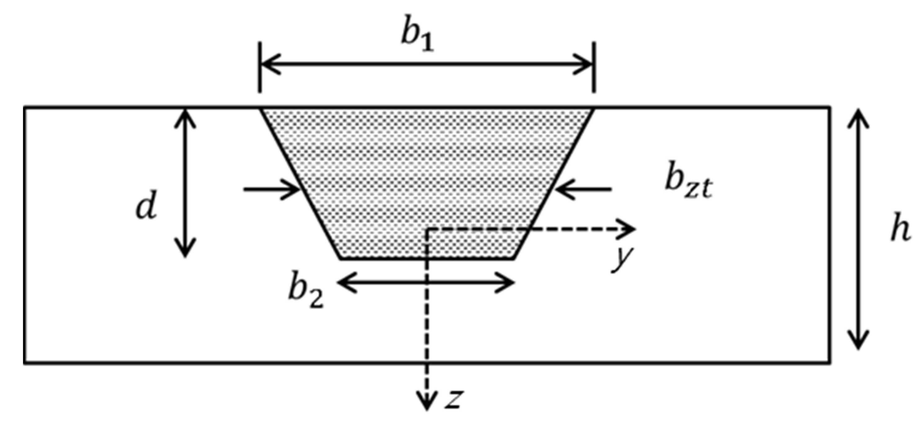
3.1. Determination of Heat Affected Zone (HAZ)

The heat affected zone is used to determine thermal deformations. Since the heat affected zone is related to phase transformation, the region can be determined based on the transformation temperature. The transformation temperature is referred to as critical temperature and is observed by measuring changes in heat transfer. The critical temperature has been developed by regression analysis of large amounts of experimental data [22]. The temperature $Ac1$ region would be suitable to determine the heat affected zone in which austenite begins to form during heating [6]. The critical temperature $T_C$ is equal to $Ac1$, which is the function of the chemical composition in steel following experimental results as shown in Equation (3) [22]. In this paper, HAZ is defined as a trapezoidal shape, as shown in Figure 5, which describes the shape variables of the trapezoidal HAZ. The shape is defined with variables: height ($h$), depth ($d$), breadth ($b1$, $b2$), as expressed as Equation (17).

$$b_{Zt}=\{\begin{array}{cc}\frac{b_2-b_1}{d}\left(Z+\frac{h}{2}\right)+b_1& z\le d-\frac{h}{2}\\ 0& d-\frac{h}{2}<z\end{array}$$

(17)

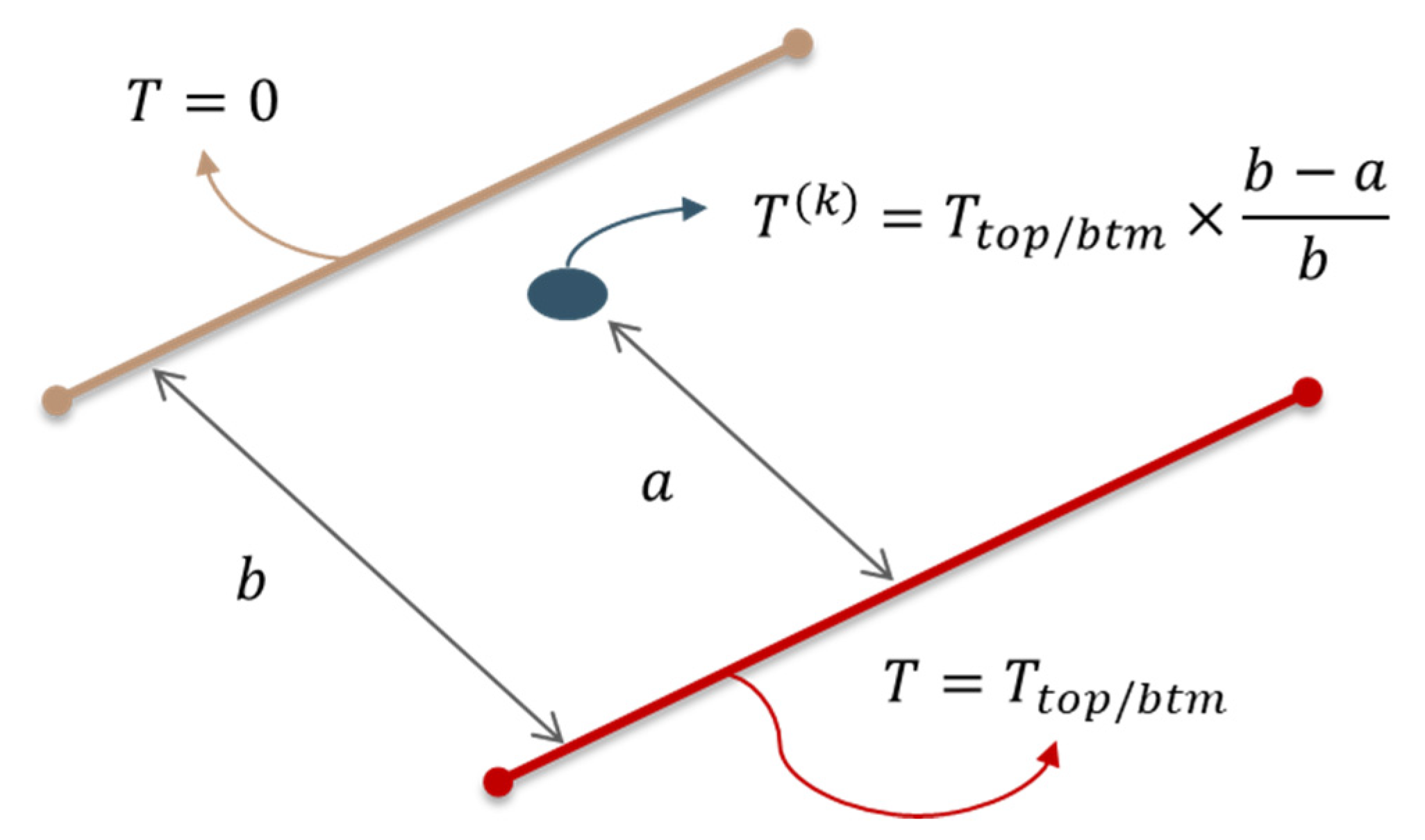
3.2. Determination of Virtual Temperature

The SDB method uses the calculated thermal strain as a direct coefficient of thermal expansion for the shell element in the finite element method (FEM) and assigns a virtual temperature, which is calculated by the dimension of the heat affected zone as shown in Equation (18) as a boundary condition. Figure 6 explains the modeling concept of the virtual temperature. The virtual temperature is applied to predict the thermal deformation, which is determined by the shape of the HAZ. Therefore, the temperature distribution of the HAZ results in thermal deformation in the FEM analysis [8].

$$T=\{\begin{array}{c}{T}_{top}=\frac{1}{b_{1}h}{\int }_{d-\frac{h}{2}}^{-\frac{h}{2}}{b}_Z\times \left(1-\frac{4}{h}\times Z\right)dZ\\ T_{btm}=\frac{1}{b_{2}h}{\int }_{d-\frac{h}{2}}^{-\frac{h}{2}}{b}_Z\times \left(1+\frac{4}{h}\times Z\right)dZ\end{array}$$

(18)

As shown in Figure 6, the size of shell elements is the same as the maximum breadth of the HAZ. If there is only one heating line, top and bottom temperature are input only at the point along the heating line, and the other points must be zeros. However, as the number of heating lines increases and overlaps with each other, it is impossible to produce elements with uniform widths. For this reason, additional virtual temperatures are required for irregular grid mesh. Through the comparison of deformation by a single heating line, it is found that the deformation results are all the same if the temperature field is the same, even if the shell element size is not equal to the breadth of HAZ. The virtual temperature for any point ($k$) can be expressed as Equation (19) [8]. The temperature of all points is equivalent to 0, and the virtual temperature calculated in Equation (19) is input only to the nodes along the heating line. By using this method, the residual stress field can be shown clearly.

$$T^{\left(k\right)}=\{\begin{array}{c}{T}_{top}^{\left(k\right)}=T_{top}\frac{b-a}{b}\\ T_{btm}^{\left(k\right)}=T_{btm}\frac{b-a}{b}\end{array}$$

(19)

where $b$ and $a$ represent the breadth of the HAZ and the straight-line distance from the heating line as shown in Figure 7, respectively.

4. Application of Method

4.1. Problem Description

The proposed methods were applied to an 18 mm thick steel curved plate with a curvature of 1/1500mm. The dimensions are length: 3000mm and width: 1500mm. A-grade mild steel was applied. As shown in Figure 8, the HAZ dimension was measured to define the shape variables. The $b_1$, $b_2$, and $d$ are 14 mm, 8 mm, and 0.6 mm, respectively, and the heating lines are 15ea, as shown in Figure 9. The heat source moving speed is 3mm/sec and sequentially heated from the left line.

4.2. Virtual Temperature Fields

The virtual temperature calculated along the heating line, as described in Equations (18) and (19), is reflected as a representative coefficient of temperature difference in the SDB method. Therefore, the calculated virtual temperature is applied as boundary conditions on the FEM model, as shown in Figure 10. It can be seen that the top- and bottom-surface temperatures were applied along the heating line, through the quasi-static FEA. The temperature distribution of Figure 10 shows the results of the application of virtual temperature coefficient according to the heating path shown in Figure 9.

4.3. Results Comparison

To compare results, an accurate comparison between the results predicted by the SBD method and the design features is required. Therefore, in order to converge data on two different coordinate systems, we applied iterative close point (ICP) algorithms [23], which are commonly used mainly for feature registration, which is a method of convergence using unit quaternion presented by Horn [24]. The ICP algorithm was commonly used for registration problems with two coordinate systems located differently. The 3D plot results of the experiment and the prediction by SDB method using shell elements are shown in Figure 11. The computational time was about 90 s, and the convergence results for comparing the experimental and predicted results are shown in Figure 11 and Figure 12. The reference point was set to four corners of the curved plate, and the tolerance was set ±3mm. The maximum difference was 9.98mm and the area within the tolerance range was 5.47% of the whole plate, with a root mean square (RMS) error of 8.89mm.

In addition, the results of the comparison by different data are described as shown in Figure 11. After matching the position of the four corners of the plate as reference points, the deformations were analyzed. The comparison results of changing the reference points are shown in Figure 12. In addition, the information of numerical results are summarized in

Table 2. Comparison of errors between the design curved shape and the shape after simulation.

Case Number	Max. [mm]	Min. [mm]	Average [mm]	RMS [mm]	Standard Deviation [mm]	Within Tolerance Range [%]
1	−17.8434	16.3479	4.7602	8.8977	7.5173	5.4656
2	−15.1433	19.5864	8.1553	11.2521	7.7526	3.4413
3	−6.6646	20.7406	11.6054	13.4235	6.7459	3.6437
4	−6.0407	21.7511	11.6627	13.7764	7.3329	2.0243
5	−6.7746	17.9434	8.1489	10.7141	6.9561	7.0850

. The case with the least root mean square error (RMS) is shown in the calculation results, and the largest ratio of area within the tolerance range is Case 5 in Figure 12d with 7.09%.

5. Conclusions

In this paper, the prediction of thermal deformation of plate by flame bending was carried out using the SDB method based on thermal strain. The phase transformation and martensite volumetric expansion induced by water cooling was considered in the SDB method. A modified thermal expansion coefficient was suggested to represent the phase transformation strain. In the SDB method, instead of elastic analysis based on inherent strain, the elastic-plastic analysis based on the modified thermal strain considering phase transformation was used to represent the additional loads effect, which was produced by previous heating lines. In this study, the shape of the inherent strain region that we have obtained through the heat transfer analysis lies between the trapezoid and the ellipse. After much experience, it is shown that the inherent strain region as a trapezoid is more suitable for the SDB method based on thermal strain to predict the thermal deformation whether in a single heating-line system or in multiple heating-line systems. In addition, in the arbitrary heating-line system, if the nodes around the heating lines are non-uniform and irregular, then the distance between the surrounding points and the heating lines, which has less spacing than the breadth of the inherent strain region, was considered to assume the proper inherent strain distribution. The results of thermal deformation in the SDB method based on thermal strain considering phase transformation showed good agreements within the error of 7%. As a result, it has been verified that the SDB method based on thermal strain can predict reasonable deformed shape, which can replace the three-dimensional thermo-elasto-plastic analysis.

In the actual flame bending (or line heating) during ship construction, more complex heating lines are imposed on the plate. Thus, the SDB method based on thermal strain considering the phase transformation can accurately and rapidly predict the thermal deformation of thick steel plate. However, in this work, we conducted a limited case study. Therefore, various case studies will be conducted on concave, saddle twist-type shapes to improve the accuracy of the prediction method.

References

1. Shin, J.G.; Lee, J.H. Nondimensionalized relationship between heating conditions and residual deformations in the line heating process. J. Ship Res. 2002, 46, 229–238. [Google Scholar] [CrossRef]
2. Shin, J.G.; Ryu, C.H.; Lee, J.H.; Kim, W.D. User-friendly, advanced line heating automation for accurate plate forming. J. Ship Prod. 2003, 19, 8–15. [Google Scholar] [CrossRef]
3. Nomoto, T.; Ohmori, T.; Sutoh, T.; Enosawa, M.; Aoyama, K.; Saitoh, M. Development of simulator for plate bending by line-heating. J. Soc. Nav. Archit. Jpn. 1990, 168, 527–535. [Google Scholar] [CrossRef]
4. Jang, C.D.; Kim, H.K.; Ha, Y.S. Prediction of plate bending by high-frequency induction heating. J. Ship Prod. 2002, 18, 226–236. [Google Scholar] [CrossRef]
5. Yu, G. Modeling of Shell Forming by Line Heating. Ph.D. Thesis, Massachusetts Institute of Technology, Massachusetts Ave., Cambridge, MA, USA, 2000. [Google Scholar]
6. Jang, C.D. A study on the prediction of deformations of plates due to line heating using a simplified thermal elasto-plastic analysis. J. Ship Prod. 1997, 13, 22–27. [Google Scholar] [CrossRef]
7. Jang, C.D.; Ha, Y.S.; Ko, D.E. An Improved Inherent Strain Analysis for the Prediction of Plate Deformations Induced by Line Heating Considering Phase Transformation of Steel. In Proceedings of the Thirteenth International Offshore and Polar Engineering Conference, Honolulu, HI, USA, 25–30 May 2003. [Google Scholar]
8. Ha, Y.S. Development of thermal distortion analysis method on large shell structure using inherent strain as boundary condition. J. Soc. Nav. Archit. Korea 2008, 45, 93–100. [Google Scholar] [CrossRef]
9. Ha, Y.S.; Jang, C.D. Developed Inherent Strain Method Considering Phase Transformation of Mild Steel in Line Heating. J. Soc. Nav. Archit. Korea 2004, 41, 65–74. [Google Scholar]
10. Ha, Y.S. A study on weldment boundary condition for elasto-plastic thermal distortion analysis of large welded structures. J. Weld. Join. 2011, 29, 48–53. [Google Scholar] [CrossRef]
11. Satoh, K.; Matsui, S.; Terai, K.; Iwamura, Y. Water-cooling effect on angular distortion caused by the process of line heating in steel plates. J. Soc. Nav. Archit. Jpn. 1969, 126, 445–458. [Google Scholar] [CrossRef]
12. Chiang, J.; Boyd, J.D.; Pilkey, A.K. Effect of microstructure on retained austenite stability and tensile behaviour in an aluminum-alloyed TRIP steel. Mater. Sci. Eng. A. 2005, 638, 132–142. [Google Scholar] [CrossRef]
13. Payson, P.; Savage, C.H. Martensitic reactions in alloy steels. Trans. ASM 1994, 33, 261–275. [Google Scholar]
14. Koistinen, D.P.; Marburger, R.E. A general equation prescribing the extent of the austenite-martensite transformation in pure iron-carbon alloys and plain carbon steels. Acta Metall. 1959, 7, 59–60. [Google Scholar] [CrossRef]
15. Steven, W. The Temperature of Martensite and Bainite in Low-alloy Steels. J. Iron Steel Inst. 1956, 183, 349–359. [Google Scholar]
16. Guo, Z.; Saunders, N.; Miodownik, P.; Schillé, J.P. Modelling phase transformations and material properties critical to the prediction of distortion during the heat treatment of steels. Int. J. Microstruct. Mater. Prop. 2009, 4, 187–195. [Google Scholar] [CrossRef]
17. Melloy, G.F. Austenite Grain Size—Its Control and Effects; Metals Engineering Institute, American Society for Metals: Metals Park, OH, USA, 1968. [Google Scholar]
18. Swarr, T.; Krauss, G. The effect of structure on the deformation of as-quenched and tempered martensite in an Fe-0.2 pct C alloy. Metall. Trans. A 1976, 7, 41–48. [Google Scholar] [CrossRef]
19. Krauss, G.; Marder, A.R. The morphology of martensite in iron alloys. Metall. Trans. 1971, 2, 2343–2357. [Google Scholar] [CrossRef]
20. Ha, Y.S.; Jang, C.D. An improved inherent strain analysis for plate bending by line heating considering phase transformation of steel. Int. J. Offshore Polar Eng. 2007, 17, ISOPE-07-17-2-139. [Google Scholar]
21. Bain, E.C.; Paxton, H.W. Alloying Elements in Steel; American Society for Metals: Cleveland, OH, USA, 1966. [Google Scholar]
22. Krauss, G. Chapter 29, Phases and Structures. In Steels: Processing, Structure, and Performance, 2nd ed.; Materials, P., Ed.; American Society for Metals: Cleveland, OH, USA, 2015; pp. 17–38. [Google Scholar]
23. Besl, P.J.; McKay, N.D. A method for registration of 3-D shapes. IEEE Tpami 1992, 14, 239–256. [Google Scholar] [CrossRef]
24. Horn, B.K. Closed-form solution of absolute orientation using unit quaternions. J. Opt. Soc. Am. A 1987, 4, 629–642. [Google Scholar] [CrossRef]
Figure 1. Stress–strain curve of heat affected zone (HAZ) [10].
Applsci 11 02011 g001
Figure 2. Phase transformation during the heating and cooling process.
Applsci 11 02011 g002
Figure 3. Austenitic grain size and ASTM number [17].
Applsci 11 02011 g003
Figure 4. Modified thermal expansion coefficient and thermal strain in cooling cycle: (a) Thermal strain; (b) Thermal expansion coefficient
Applsci 11 02011 g004
Figure 5. Trapezoid shape heat affected zone (HAZ).
Applsci 11 02011 g005
Figure 6. Temperature boundary conditions imposed on the shell element.
Applsci 11 02011 g006
Figure 7. Virtual temperature for irregular mesh.
Applsci 11 02011 g007
Figure 8. HAZ shape obtained by experimental heating.
Applsci 11 02011 g008
Figure 9. Heating paths applied to experimental case.
Applsci 11 02011 g009
Figure 10. Temperature deviation coefficient in virtual temperature fields. (a) Top surface; (b) Bottom surface.
Applsci 11 02011 g010
Figure 11. Coordination reference shape and target shape (Case 1).
Applsci 11 02011 g011
Figure 12. Comparisons of experimental result and predictive result with different reference points. (a) Case 2; (b) Case 3; (c) Case 4; (d) Case 5.
Applsci 11 02011 g012