Computation of Effective Elastic Properties Using a Three-Dimensional Semi-Analytical Approach for Transversely Isotropic Nanocomposites

Abstract

A three-dimensional semi-analytical finite element method (SAFEM-3D) is implemented in this work to calculate the effective properties of periodic elastic-reinforced nanocomposites. Different inclusions are also considered, such as discs, ellipsoidals, spheres, carbon nanotubes (CNT) and carbon nanowires (CNW). The nanocomposites are assumed to have isotropic or transversely isotropic inclusions embedded in an isotropic matrix. The SAFEM-3D approach is developed by combining the two-scale asymptotic homogenization method (AHM) and the finite element method (FEM). Statements regarding the homogenized local problems on the periodic cell and analytical expressions of the effective elastic coefficients are provided. Homogenized local problems are transformed into boundary problems over one-eighth of the cell. The FEM is implemented based on the principle of the minimum potential energy. The three-dimensional region (periodic cell) is divided into a finite number of 10-node tetrahedral elements. In addition, the effect of the inclusion’s geometrical shape, volume fraction and length on the effective elastic properties of the composite with aligned or random distributions is studied. Numerical computations are developed and comparisons with other theoretical results are reported. A comparison with experimental values for CNW nanocomposites is also provided, and good agreement is obtained.

1. Introduction

Single-walled carbon nanotube (SWNT) composites embedded in a polymer matrix are called nanocomposite materials. They show superior mechanical, thermal and processing properties in comparison with other materials that do not have reinforcement. Nanocomposite materials are suitable for aerospace, automotive, aeronautic and sporting goods applications [1,2,3,4]. Current global expectations regarding the creation of high-performance, lightweight and low cost products requires the design of specific properties [5,6]. In this sense, the effective property estimation of multi-phase composites, based on a technological approach supported by modeling and numerical simulation, allows a better understanding and analysis of new materials with higher standards, as well as reducing costs and production times [7,8,9,10]. The effective properties of nanocomposites are influenced by factors such as their structure, orientation, dispersion, fiber diameter and matrix stiffness [11,12,13,14]. Different techniques have been developed to study the elastic behavior of multi-phase fiber-reinforced composites (FRCs) [15,16].

Homogenization techniques have always been a useful tool to describe the structure–property relationship of composite materials [17,18,19,20,21]. For example, Bravo-Castillero et al. [22] determined the effective properties of elastic FRCs with square and hexagonal fiber distributions by means of the asymptotic homogenization method (AHM) for bone mechanics applications. Rodríguez-Ramos et al. [23] calculated the effective properties of elastic FRCs with transverse isotropic constituents and parallelogram-like periodic unit cells using the AHM. Zhao et al. [24] predicted the effective elastic properties of polymer nanocomposites using a novel numerical implementation of AHM. Baek et al. [25] proposed a two-step homogenization approach to analyze the mechanical behavior of polymeric nanocomposites based on multiscale homogenization and the clustering density concept. In the literature, different homogenization implementations and computer modeling techniques to predict the effective properties of nanocomposites can be found; see for instance [26,27,28]. They represent a rewarding advantage through validations by comparing different models.

In addition, Otero et al. [29] proposed a semi-analytical method to find the effective coefficients of elastic FRCs with aligned inclusions and transversely isotropic constituents. An extension of this 2D semi-analytical method for coupled field problems was reported by Espinosa-Almeyda et al. [30]. Gabbert et al. [31] developed a semi-analytical approach based on FEM linked with the homogenization method to solve the inverse problem to determine microscale distributions. Nasution et al. [32] presented a new asymptotic expansion homogenization model to study the thermodynamic properties of 3D composites. In their work, the mathematical treatment takes into account the benefits of 2D homogenization and periodicity in the in-plane direction. The mechanical behaviors of three-dimensional short fiber composites, including interface debonding, were studied using an extended finite-element method (XFEM) [33]. Fisher et al. [34,35] studied the effect of carbon nanotube (CNT) inclusions on the effective elastic properties of composites by numerical simulation techniques, using finite elements coupled with the Mori–Tanaka model. A computational approach based on FEM was implemented to predict the elastic behavior of a hybrid nanocomposite reinforced by CNTs and nano-clay platelets in an epoxy system [36]. A review of FEM applications in the analysis of composite materials was reported in [37]. More recently, many research works have reported on the field of nanocomposites reinforced by CNT inclusions; for example, Tarfaoui et al. [38] analyzed the effect of CNT additives on the mechanical behavior of three-phase polymer-matrix composites by experimental techniques. Choi et al. [39] proposed a multi-scale method to obtain the mechanical properties of interfacial regions of SWNT/epoxy nanocomposites. E. Moumen et al. [40] estimated the elastic properties of laminated composites reinforced by CNT using a numerical homogenization approach, and comparisons with experimental data were reported. A review of the most important and novel theoretical and experimental methods applied to study the mechanical behavior of 1D, 2D and 3D CNT-reinforced nanocomposites was presented in [41].

In this work, the effective coefficients of periodic multi-phase elastic FRCs are calculated by the three-dimensional semi-analytical finite element method (SAFEM-3D). Herein, the elastic reinforced nanocomposites are assumed to have isotropic or transversely isotropic CNT inclusions within an isotropic matrix. The SAFEM-3D approach is based on a combination of the AHM and the finite element method (FEM). Using the AHM, the homogenized local problems are stated and the analytical expressions of the effective elastic properties are obtained. The FEM allows local problems to be solved via the minimum potential energy principle. Local problems over the unit cell are transformed into boundary problems over one-eighth of the unit cell. Numerical values are reported for different nanocomposite materials with an aligned or random distribution of the inclusions. The effective coefficients of periodic elastic FRCs with different inclusions in the form of discs, ellipsoidals, spheres, carbon nanotubes (CNT) and carbon nanowires (CNW) are calculated. The effect of the inclusion geometry shape, volume fraction and inclusion length on the effective elastic properties is analyzed. Comparisons with some theoretical methods and experimental data reported in the literature show good agreements.

2. Statement of the Problem for Heterogeneous Media

A heterogeneous medium occupying a volume $\Omega \in {\mathfrak{R}}^3$ with a boundary $\partial \Omega ={\partial }_1\Omega \cup {\partial }_2\Omega$ is considered as a periodic two-phase elastic FRC (inclusion/matrix) at the Cartesian coordinate system $\mathbf{x}=(x_1,x_2,x_3)$ (see Figure 1). In particular, an elastic FRC with transversely isotropic CNT inclusions embedded into an isotropic matrix is studied. The CNT’s inclusions have a periodic distribution along the axes $O{x}_1$, $O{x}_2$ and $O{x}_3$ without overlapping within the homogeneous matrix. The periodic unit cell S is taken as a cubic matrix with a centered CNT inclusion in the form of discs, spheres, ellipsoids and hollow cylinders at the Cartesian coordinate system $\mathbf{y}=(y_1,y_2,y_3)$. The regions occupied by the matrix $S_1$ with volume $V_1$ and the CNT inclusions $S_2$ with volume $V_2$ satisfy that $S=S_1\cup S_2$ with $S_1\cap S_2=\varnothing$, and the unit cell volume is $V=V_1+V_2$. Perfect contact conditions between the matrix and the inclusions are assumed; that is, mechanical displacements and stresses are continuous across the interface, denoted by $\Gamma$ (see, for instance, [23]). The values associated with the matrix and the inclusion are indicated by superscripts in parentheses $\left(2\right)$ and $\left(1\right)$, respectively.

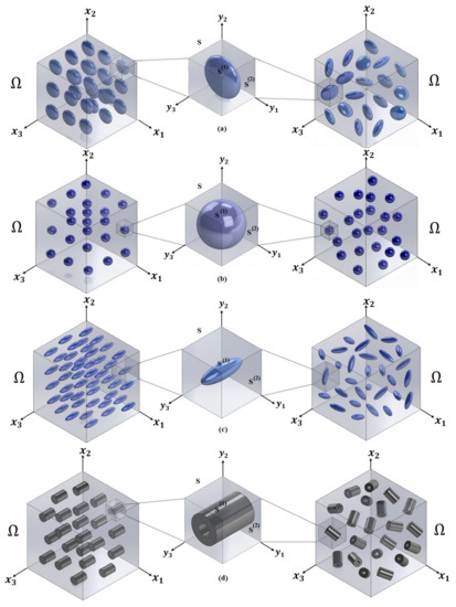
Figure 1. Representative section of a two-phase composite material reinforced by aligned (left) and random (right) inclusions. Three-dimensional periodic cell (middle) with different inclusion shapes: discs (a), spheres (b), ellipsoids (c) and hollow cylinders (d).

The static governing equations for a heterogeneous multi-phase elastic composite associated with the theory of linear elasticity [42,43] are defined by

$$\frac{\partial {\sigma }_{ij}}{\partial x_j}=0,\mathrm{in}\Omega ,$$

(1)

together with the boundary conditions

$$\begin{array}{cc}\hfill u_i& =0,\mathrm{on}{\partial }_1\Omega ,\hfill \\ \hfill {\sigma }_{ij}{n}_j& =0,\mathrm{on}{\partial }_2\Omega ,\hfill \end{array}$$

(2)

where $i,j=1,2,3$ and ${\sigma }_{ij}$ and $u_i$ represent the components of the second-order stress tensor and the displacement vector, respectively. In addition, $n_j$ is the normal unit vector to ${\partial }_2\Omega$.

Furthermore, the constitutive equations are defined by Hooke’s law:

$${\sigma }_{ij}=C_{ijkl}\left(\mathbf{x}\right){\epsilon }_{kl},$$

(3)

where $C_{ijkl}$$(k,l=1,2,3)$ is the elasticity modulus and ${\epsilon }_{kl}$ represents the strain components, such as

$${\epsilon }_{kl}=\frac{1}{2}\left(\frac{\partial u_k}{\partial x_l}+\frac{\partial u_l}{\partial x_k}\right).$$

(4)

Besides, the perfect contact conditions between the matrix and inclusion phases are assumed:

$$u_i^{\left(1\right)}{\mid }_{\Gamma }=u_i^{\left(2\right)}{\mid }_{\Gamma },{\sigma }_{ij}^{\left(1\right)}{n}_j^{\left(1\right)}{\mid }_{\Gamma }={\sigma }_{ij}^{\left(2\right)}{n}_j^{\left(2\right)}{\mid }_{\Gamma }.$$

(5)

3. Asymptotic Homogenization Method: Homogeneous Problem, Local Problems and Effective Coefficients

The homogenized local problems over S, the homogeneous static problem and effective coefficients linked to the periodic elastic FRC are derived from Equations (1)–(5) using the AHM [17,22,23] by means of the asymptotic expansion of the displacement $u_i$ in powers of the parameter $ϵ$, resulting in the following:

$$u_i=u_i^{\left(0\right)}\left(\mathbf{x}\right)+ϵu_i^{\left(1\right)}(\mathbf{x},\mathbf{y})+{ϵ}^2{u}_i^{\left(2\right)}(\mathbf{x},\mathbf{y})+\cdots ,$$

(6)

where $u_i^{\left(0\right)}$ is a function only of the slow variable $\mathbf{x}$, $u_i^{\left(k\right)}(\mathbf{x},\mathbf{y})$$(k=1,2,\cdots )$ are S-periodic functions with respect to the fast variable $\mathbf{y}$ and the superscripts denote the order of terms in the expansions. Here, the two-scales, denoted by $\mathbf{x}$ (global or slow) and $\mathbf{y}$ (local or fast), characterize the global behavior of the composite and the heterogeneities at a local level over S, respectively. The scales are related by $\mathbf{y}=\mathbf{x}/ϵ$, where $ϵ$ is a small enough parameter which represents the ratio between the dimensions of the periodic cell S and the characteristic dimensions of the nanocomposite.

The mathematical statement of the ${}_{pq}L$ local problems over the unit cell S are stated as

$$\frac{\partial {}_{pq}{\tau }_{ij}\left(\mathbf{y}\right)}{\partial y_j}=-\frac{\partial C_{ijpq}\left(\mathbf{y}\right)}{\partial y_j},$$

(7)

subject to the perfect interface conditions, as shown in Equation (5), which in this case are

$${}_{pq}{N}_k^{\left(1\right)}\left(\mathbf{y}\right)={}_{pq}{N}_k^{\left(2\right)}\left(\mathbf{y}\right)\mathrm{on}\Gamma$$

(8)

$$C_{ijpq}^{\left(1\right)}\left(\mathbf{y}\right)+{}_{pq}{\tau }_{ij}^{\left(1\right)}\left(\mathbf{y}\right)n_j^{\left(1\right)}=C_{ijpq}^{\left(2\right)}\left(\mathbf{y}\right)+{}_{pq}{\tau }_{ij}^{\left(2\right)}\left(\mathbf{y}\right)n_j^{\left(2\right)},\mathrm{on}\Gamma$$

(9)

where the components of the Y-periodic local stress tensor are

$${}_{pq}{\tau }_{ij}\left(\mathbf{y}\right)=C_{ijkl}\left(\mathbf{y}\right)\frac{{\partial }_{pq}{N}_k\left(\mathbf{y}\right)}{\partial y_l}.$$

(10)

and ${}_{pq}{N}_k$$(k,p,q=1,2,3)$ are the components of the S-periodic local pseudo-displacements vector, providing the solution of the ${}_{pq}L$ local problems. Additionally, the following condition, over S, is needed to guarantee a unique solution of the local problems: ${⟨}_{pq}{N}_k⟩=0$. Here, $⟨·⟩=(1/|S\left|\right)\int (·)d\mathbf{y}$ is the average operator over the periodic cell S and $\left|S\right|$ is the volume of the cell.

The homogeneous static problem equivalent to Equation (1) is stated as follows:

$$\frac{\partial {\overline{\sigma }}_{ij}^{\left(0\right)}\left(\mathbf{x}\right)}{\partial x_j}=0,$$

(11)

where the constitutive equations of the homogeneous problem are

$${\overline{\sigma }}_{ij}^{\left(0\right)}\left(\mathbf{x}\right)=⟨{\sigma }_{ij}^{\left(0\right)}\left(\mathbf{x}\right)⟩=C_{ijpq}^{\ast }\frac{\partial u_p^{\left(0\right)}\left(\mathbf{x}\right)}{\partial x_q},$$

(12)

where $u_p^{\left(0\right)}\left(\mathbf{x}\right)$ is the solution of the homogenized problem in Equation (11) and $C_{ijpq}^{\ast }$ are the effective coefficients, which are defined as follows:

$$C_{ijpq}^{\ast }=⟨C_{ijpq}\left(\mathbf{y}\right)+{}_{pq}{\tau }_{ij}\left(\mathbf{y}\right)⟩.$$

(13)

The boundary conditions expressed in Equation (2) are transformed into

$$\begin{array}{c}\hfill u_i^{\left(0\right)}\left(\mathbf{x}\right)=0,\mathrm{on}{\partial }_1\Omega ,\\ \hfill {\overline{\sigma }}_{ij}^{\left(0\right)}\left(\mathbf{x}\right)n_j=0,\mathrm{on}{\partial }_2\Omega .\end{array}$$

(14)

The mathematical procedures to obtain the ${}_{pq}L$ local problems (Equations (7)–(10)) and the homogeneous static problem (Equations (11)–(12)) can be seen in Appendix A. More details explaining he AHM procedure and the rigorous theoretical mathematical background can be found in the classical works [17,20,44,45].

Six local problems ${}_{pq}L$$(p,q=1,2,3)$ in terms of the local variable $\mathbf{y}$ are defined in the unit cell S. Each problem is decoupled into an independent set of equations according to the plane and out-of-plane deformation state assumed in linear elasticity. Table 1 shows the correspondence between the effective elastic coefficients and the local problems ${}_{pq}L$.

Table 1. Local problems and associated effective coefficients.

${}_{11}\mathit{L}$	${}_{22}\mathit{L}$	${}_{33}\mathit{L}$	${}_{23}\mathit{L}$	${}_{13}\mathit{L}$	${}_{12}\mathit{L}$
$C_{1111}^{\ast }$	$C_{1122}^{\ast }$	$C_{1133}^{\ast }$	0	0	0
$C_{2211}^{\ast }$	$C_{2222}^{\ast }$	$C_{2233}^{\ast }$	0	0	0
$C_{3311}^{\ast }$	$C_{3322}^{\ast }$	$C_{3333}^{\ast }$	0	0	0
0	0	0	$C_{2323}^{\ast }$	0	0
0	0	0	0	$C_{1313}^{\ast }$	0
0	0	0	0	0	$C_{1212}^{\ast }$

The local problems can be presented as follows:

Problems ${}_{\lambda 3}L$ with $\lambda ,\beta =1,2$ and $\lambda \ne \beta :$

$$\begin{array}{cc}\hfill \frac{{\partial }_{\lambda 3}{\tau }_{\lambda 1}}{\partial y_1}+\frac{{\partial }_{\lambda 3}{\tau }_{\lambda 2}}{\partial y_2}+\frac{{\partial }_{\lambda 3}{\tau }_{\lambda 3}}{\partial y_3}& =-\frac{\partial C_{\lambda 3\lambda 3}}{\partial y_3},\hfill \\ \hfill \frac{{\partial }_{\lambda 3}{\tau }_{31}}{\partial y_1}+\frac{{\partial }_{\lambda 3}{\tau }_{32}}{\partial y_2}+\frac{{\partial }_{\lambda 3}{\tau }_{33}}{\partial y_3}& =-\frac{\partial C_{3\lambda \lambda 3}}{\partial y_{\lambda }},\hfill \\ \hfill \frac{{\partial }_{\lambda 3}{\tau }_{\beta 1}}{\partial y_1}+\frac{{\partial }_{\lambda 3}{\tau }_{\beta 2}}{\partial y_2}+\frac{{\partial }_{\lambda 3}{\tau }_{\beta 3}}{\partial y_3}& =0.\hfill \end{array}$$

(15)

Problems ${}_{\beta \beta }L$ with $\beta =1,2,3:$

$$\begin{array}{cc}\hfill \frac{{\partial }_{\beta \beta }{\tau }_{11}}{\partial y_1}+\frac{{\partial }_{\beta \beta }{\tau }_{12}}{\partial y_2}+\frac{{\partial }_{\beta \beta }{\tau }_{13}}{\partial y_3}& =-\frac{\partial C_{11\beta \beta }}{\partial y_1},\hfill \\ \hfill \frac{{\partial }_{\beta \beta }{\tau }_{21}}{\partial y_1}+\frac{{\partial }_{\beta \beta }{\tau }_{22}}{\partial y_2}+\frac{{\partial }_{\beta \beta }{\tau }_{23}}{\partial y_3}& =-\frac{\partial C_{22\beta \beta }}{\partial y_2},\hfill \\ \hfill \frac{{\partial }_{\beta \beta }{\tau }_{31}}{\partial y_1}+\frac{{\partial }_{\beta \beta }{\tau }_{32}}{\partial y_2}+\frac{{\partial }_{\beta \beta }{\tau }_{33}}{\partial y_3}& =-\frac{\partial C_{33\beta \beta }}{\partial y_3}.\hfill \end{array}$$

(16)

Problem ${}_{12}L:$

$$\begin{array}{cc}\hfill \frac{{\partial }_{12}{\tau }_{11}}{\partial y_1}+\frac{{\partial }_{12}{\tau }_{12}}{\partial y_2}+\frac{{\partial }_{12}{\tau }_{13}}{\partial y_3}& =-\frac{\partial C_{1212}}{\partial y_2},\hfill \\ \hfill \frac{{\partial }_{12}{\tau }_{21}}{\partial y_1}+\frac{{\partial }_{12}{\tau }_{22}}{\partial y_2}+\frac{{\partial }_{12}{\tau }_{23}}{\partial y_3}& =-\frac{\partial C_{2112}}{\partial y_1},\hfill \\ \hfill \frac{{\partial }_{12}{\tau }_{31}}{\partial y_1}+\frac{{\partial }_{12}{\tau }_{32}}{\partial y_2}+\frac{{\partial }_{12}{\tau }_{33}}{\partial y_3}& =0.\hfill \end{array}$$

(17)

In the Equations (15)–(17), the elastic coefficients $C_{ijkl}\left(\mathbf{y}\right)=C_{ijkl}(y_1,y_2,y_3)$ are assumed to be even functions with respect to the variables $y_1$, $y_2$ and $y_3$. Then, the following conditions are satisfied:

$${}_{pq}{N}_i{\mid }_{y_h=d_h}=0,\mathrm{if}{\delta }_{hi}+{\delta }_{hp}+{\delta }_{hq}\mathrm{is}\mathrm{odd},$$

(18)

$${}_{pq}{\tau }_i{\mid }_{y_h=d_h}=0,\mathrm{if}{\delta }_{hi}+{\delta }_{hp}+{\delta }_{hq}+1\mathrm{is}\mathrm{even},$$

(19)

where $d_h=\{0,l_h\}$$(h=1,2,3)$, $l_h$ is the semi-length of the cell in the $y_h$ direction and the function ${\delta }_{hi}$ is defined as follows:

$${\delta }_{hi}=\left\{\begin{array}{cc}1\hfill & \mathrm{if}h=i,\hfill \\ 0\hfill & \mathrm{if}h\ne i.\hfill \end{array}\right.$$

(20)

The local problems ${}_{pq}L$ over S can be transformed into boundary problems over one-eighth of the periodic unit cell S by applying the conditions in Equations (18) and (19) [46]. Thus, the local functions are related to the new variable ${}_{pq}{M}_k$ as follows:

$${}_{pq}{N}_k={}_{pq}{M}_k-y_p{\delta }_{kq},$$

(21)

where $p,q,l=1,2,3$.

From Equations (7), (10) and (11), the following relations can be obtained:

$${}_{pq}{\tau }_k\left(\mathbf{y}\right)={}_{pq}{\sigma }_{ij}\left(\mathbf{y}\right)-C_{ijpq}\left(\mathbf{y}\right),$$

(22)

$${}_{pq}{\sigma }_{ij}\left(\mathbf{y}\right)=C_{ijkl}\left(\mathbf{y}\right)\frac{{\partial }_{pq}{M}_k\left(\mathbf{y}\right)}{\partial y_l},$$

(23)

$$\frac{{\partial }_{pq}{\sigma }_{ij}\left(\mathbf{y}\right)}{\partial y_j}=0,$$

(24)

and the effective elastic coefficients shown by Equation (13) can be expressed as

$$C_{ijpq}^{\ast }=8{⟨}_{pq}{\sigma }_{ij}\left(\mathbf{y}\right)⟩.$$

(25)

The local problems ${}_{pq}L$ can be restated as equivalent boundary value local problems ${}_{pq}L$ over one-eighth of the cell S as follows:

$$\begin{array}{cc}\hfill \frac{{\partial }_{pq}{\sigma }_{11}^{({\rm Y})}}{\partial y_1}+\frac{{\partial }_{pq}{\sigma }_{12}^{({\rm Y})}}{\partial y_2}+\frac{{\partial }_{pq}{\sigma }_{13}^{({\rm Y})}}{\partial y_3}& =0,\hfill \\ \hfill \frac{{\partial }_{pq}{\sigma }_{21}^{({\rm Y})}}{\partial y_1}+\frac{{\partial }_{pq}{\sigma }_{22}^{({\rm Y})}}{\partial y_2}+\frac{{\partial }_{pq}{\sigma }_{23}^{({\rm Y})}}{\partial y_3}& =0,\hfill \\ \hfill \frac{{\partial }_{pq}{\sigma }_{31}^{({\rm Y})}}{\partial y_1}+\frac{{\partial }_{pq}{\sigma }_{32}^{({\rm Y})}}{\partial y_2}+\frac{{\partial }_{pq}{\sigma }_{33}^{({\rm Y})}}{\partial y_3}& =0,\hfill \end{array}$$

(26)

where

$${}_{pq}{\sigma }_{\beta \beta }^{({\rm Y})}=C_{\beta \beta 11}^{({\rm Y})}\frac{{\partial }_{pq}{M}_1^{({\rm Y})}}{\partial y_1}+C_{\beta \beta 22}^{({\rm Y})}\frac{{\partial }_{pq}{M}_2^{({\rm Y})}}{\partial y_2}+C_{\beta \beta 33}^{({\rm Y})}\frac{{\partial }_{pq}{M}_3^{({\rm Y})}}{\partial y_3},$$

(27)

$${}_{pq}{\sigma }_{\lambda 3}^{({\rm Y})}={}_{pq}{\sigma }_{3\lambda }^{({\rm Y})}=C_{\lambda 3\lambda 3}^{({\rm Y})}\left(\frac{{\partial }_{pq}{M}_3^{({\rm Y})}}{\partial y_{\lambda }}+\frac{{\partial }_{pq}{M}_{\lambda }^{({\rm Y})}}{\partial y_3}\right),$$

(28)

$${}_{pq}{\sigma }_{12}^{({\rm Y})}={}_{pq}{\sigma }_{21}^{({\rm Y})}=C_{1212}^{({\rm Y})}\left(\frac{{\partial }_{pq}{M}_2^{({\rm Y})}}{\partial y_1}+\frac{{\partial }_{pq}{M}_1^{({\rm Y})}}{\partial y_2}\right),$$

(29)

where $\beta \beta =11,22,33$ and $\lambda ,{\rm Y}=1,2$. The boundary conditions associated with the boundary value local problems over one-eighth of S are summarized in Appendix B.

The effective coefficients are calculated with Equation (25) and they are listed according to the relevant problem as follows:

Problems ${}_{\beta \beta }L$ $(\beta \beta =11,22,33):$

$$C_{11\beta \beta }^{\ast }=8⟨C_{1111}\frac{{\partial }_{\beta \beta }{M}_1}{\partial y_1}+C_{1122}\frac{{\partial }_{\beta \beta }{M}_2}{\partial y_2}+C_{1133}\frac{{\partial }_{\beta \beta }{M}_3}{\partial y_3}⟩,$$

(30)

$$C_{22\beta \beta }^{\ast }=8⟨C_{1122}\frac{{\partial }_{\beta \beta }{M}_1}{\partial y_1}+C_{2222}\frac{{\partial }_{\beta \beta }{M}_2}{\partial y_2}+C_{2233}\frac{{\partial }_{\beta \beta }{M}_3}{\partial y_3}⟩,$$

(31)

$$C_{33\beta \beta }^{\ast }=8⟨C_{1133}\frac{{\partial }_{\beta \beta }{M}_1}{\partial y_1}+C_{2233}\frac{{\partial }_{\beta \beta }{M}_2}{\partial y_2}+C_{3333}\frac{{\partial }_{\beta \beta }{M}_3}{\partial y_3}⟩.$$

(32)

Problem ${}_{23}L$

$$C_{2323}^{\ast }=8⟨C_{2323}\left(\frac{{\partial }_{23}{M}_3}{\partial y_2}+\frac{{\partial }_{23}{M}_2}{\partial y_3}\right)⟩.$$

(33)

Problem ${}_{13}L$

$$C_{1313}^{\ast }=8⟨C_{1313}\left(\frac{{\partial }_{13}{M}_3}{\partial y_1}+\frac{{\partial }_{13}{M}_1}{\partial y_3}\right)⟩.$$

(34)

Problem ${}_{12}L$

$$C_{1212}^{\ast }=8⟨C_{1212}\left(\frac{{\partial }_{12}{M}_1}{\partial y_2}+\frac{{\partial }_{12}{M}_2}{\partial y_1}\right)⟩.$$

(35)

Note that the local problems subject to periodic conditions on the cell (S) (Equations (7)–(10)) are transformed into boundary problems ((Equations (26)–(29)) on one-eighth of S, considering the symmetries of the cell through Equation (21). The boundary conditions are given in Appendix B. The FEM implementation via the minimum potential energy principle for the boundary problems is explained in the following section.

Solution of Local Problems through the Finite Element Method

For many cases of FRCs with complex geometrical structures, the determination of analytical solutions for the local problems and the exact expressions of the effective coefficients through the analytic AHM are difficult or even impossible to solve. Only for specific inclusion geometries, the exact analytical solutions have been reported; see for instance [23]. In this sense, an alternative approach is the finite element method. In the present work, the SAFEM-3D approach is developed to find the solution for the local problems and the effective elastic properties. The SAFEM-3D is implemented by combining the AHM and the FEM; i.e., the local problems obtained by the AHM are solved using the FEM through the minimum potential energy principle, in a similar manner to the methodology developed by Otero et al. [29,46] applied to a bi-dimensional elastic two-phase FRC.

The total corresponding potential energy $\Pi$ for an elastic solid medium $\Omega$—see for instance [47]—is defined as

$$\Pi =\frac{1}{2}{\int }_V{\mathit{\sigma }}^T\mathit{\epsilon }dV-{\int }_V{\mathit{u}}^T\mathit{f}dV-{\int }_S{\mathit{u}}^T\mathit{T}dS-\sum _i{u}_i{P}_i,$$

(36)

where $\Pi$ involves the deformation energy per unit volume of the body and the potential energies associated with the body forces $\mathit{f}$, tensile forces $\mathit{T}$ and point loads $P_i$ respectively. In the present work, the forces $\mathit{f}$ and $\mathit{T}$ and loads $P_i$ are assumed to be zero.

The relationships given by Equations (26)–(29) are related as follows:

$${}_{pq}\mathit{\sigma }=\mathbf{D}{}_{pq}\mathit{\epsilon },$$

(37)

where

$${}_{pq}\mathit{\sigma }={\left[{}_{pq}{\sigma }_{11}{}_{pq}{\sigma }_{22}{}_{pq}{\sigma }_{33}{}_{pq}{\sigma }_{23}{}_{pq}{\sigma }_{13}{}_{pq}{\sigma }_{21}\right]}^T,$$

(38)

$$\begin{array}{cc}\hfill {}_{pq}\mathit{\epsilon }=[{}_{pq}{\epsilon }_{11}{}_{pq}{\epsilon }_{22}{}_{pq}{\epsilon }_{33}& {}_{pq}{\epsilon }_{23}{}_{pq}{\epsilon }_{13}{}_{pq}{\epsilon }_{21}{]}^T\hfill \\ \hfill =[\frac{{\partial }_{pq}{M}_1}{\partial y_1}\frac{{\partial }_{pq}{M}_2}{\partial y_2}\frac{{\partial }_{pq}{M}_3}{\partial y_3}\frac{{\partial }_{pq}{M}_2}{\partial y_3}+\frac{{\partial }_{pq}{M}_3}{\partial y_2}& \frac{{\partial }_{pq}{M}_1}{\partial y_3}+\frac{{\partial }_{pq}{M}_3}{\partial y_1}\frac{{\partial }_{pq}{M}_1}{\partial y_2}+\frac{{\partial }_{pq}{M}_2}{\partial y_1}{]}^T,\hfill \end{array}$$

(39)

and

$$\mathbf{D}=\left[\begin{array}{cccccc}{C}_{1111}& C_{1122}& C_{1133}& 0& 0& 0\\ C_{1122}& C_{2222}& C_{2233}& 0& 0& 0\\ C_{1133}& C_{2233}& C_{3333}& 0& 0& 0\\ 0& 0& 0& C_{2323}& 0& 0\\ 0& 0& 0& 0& C_{1313}& 0\\ 0& 0& 0& 0& 0& C_{1212}\end{array}\right].$$

(40)

The region of study (one-eighth of the unit cell S) is divided into a finite number of tetrahedral elements. Each element is characterized by 10 nodes located at the vertices, and the remaining ones are at the midpoints of the edges. Additionally, each node is associated with a pseudo-displacement vector connected with the ${}_{pq}L$ local problem to be solved. The pseudo-displacements ${}_{pq}{M}_k$ are defined as a linear combination of the shape functions ${\Psi }_i$ whose coefficients are the nodal values of the unknown pseudo-displacement ${}_{pq}{w}_{k\left(s\right)}$, i.e.,

$${}_{pq}{M}_k={\Psi }_s{}_{pq}{w}_{k\left(s\right)},$$

(41)

where ${}_{pq}{w}_{k\left(s\right)}$ represents the k-th component of the pseudo-displacement at the s-th node $(s=1,\cdots ,10)$ for the local problem ${}_{pq}L$.

The shape functions ${\Psi }_i$ are defined through natural coordinates [48], as follows:

$$\begin{array}{cc}\hfill {\Psi }_1& ={\xi }_1(2{\xi }_1-1),{\Psi }_2={\xi }_2(2{\xi }_2-1),{\Psi }_3={\xi }_3(2{\xi }_3-1),{\Psi }_4={\xi }_4(2{\xi }_4-1),\hfill \\ \hfill {\Psi }_5& =4{\xi }_1{\xi }_2,{\Psi }_6=4{\xi }_2{\xi }_3,{\Psi }_7=4{\xi }_3{\xi }_1,{\Psi }_8=4{\xi }_1{\xi }_4,{\Psi }_9=4{\xi }_2{\xi }_4,{\Psi }_{10}=4{\xi }_3{\xi }_4,\hfill \end{array}$$

(42)

where ${\xi }_1$,${\xi }_2$,${\xi }_3$ and ${\xi }_4=1-{\xi }_1-{\xi }_2-{\xi }_3$ represent the element’s natural coordinates. The element node vector ${}_{pq}\mathbf{w}$ is defined as

$${}_{pq}{\mathbf{w}}_{30\times 1}={\left[{}_{pq}{w}_{1\left(1\right)}{}_{pq}{w}_{2\left(1\right)}{}_{pq}{w}_{3\left(1\right)}\cdots {}_{pq}{w}_{1\left(10\right)}{}_{pq}{w}_{2\left(10\right)}{}_{pq}{w}_{3\left(10\right)}\right]}^T.$$

(43)

Taking into account Equations (41) and (42), the relationship between deformations and pseudo-displacements as shown in Equation (39) can be written in matrix form as functions of the natural coordinates and the element’s shape functions, as follows:

$${}_{\mathit{pq}}\mathit{\epsilon }=\mathbf{B}{}_{pq}\mathbf{w},$$

(44)

where $\mathbf{B}$ is the element strain–displacement matrix:

$${\mathbf{B}}_{6\times 30}=\left[\begin{array}{ccccccccc}{\mathfrak{I}}_{11}& {\mathfrak{I}}_{12}& {\mathfrak{I}}_{13}& 0& 0& 0& 0& 0& 0\\ 0& 0& 0& {\mathfrak{I}}_{21}& {\mathfrak{I}}_{22}& {\mathfrak{I}}_{23}& 0& 0& 0\\ 0& 0& 0& 0& 0& 0& {\mathfrak{I}}_{31}& {\mathfrak{I}}_{32}& {\mathfrak{I}}_{33}\\ 0& 0& 0& {\mathfrak{I}}_{31}& {\mathfrak{I}}_{32}& {\mathfrak{I}}_{33}& {\mathfrak{I}}_{21}& {\mathfrak{I}}_{22}& {\mathfrak{I}}_{23}\\ {\mathfrak{I}}_{31}& {\mathfrak{I}}_{32}& {\mathfrak{I}}_{33}& 0& 0& 0& {\mathfrak{I}}_{11}& {\mathfrak{I}}_{12}& {\mathfrak{I}}_{13}\\ {\mathfrak{I}}_{21}& {\mathfrak{I}}_{22}& {\mathfrak{I}}_{23}& {\mathfrak{I}}_{11}& {\mathfrak{I}}_{12}& {\mathfrak{I}}_{13}& 0& 0& 0\end{array}\right]{\mathbf{H}}_{9\times 30},$$

(45)

${\mathfrak{I}}_{ij}$ represent the inverse matrix coefficients of the Jacobian transformation $\mathbf{J}$ between the Cartesian system $(y_1,y_2,y_3)$ and the natural coordinate system $({\xi }_1,{\xi }_2,{\xi }_3)$, and the matrix ${\mathbf{H}}_{9\times 30}$ is defined in Appendix C.

The stress values are determined as functions of the natural coordinates and the element’s shape functions by means of the relations shown in Equations (37)–(42), such that

$${}_{pq}\mathit{\sigma }=\mathbf{DB}{}_{pq}\mathbf{w}.$$

(46)

Replacing Equations (44) and (46) into Equation (36), we obtain the deformation energy ${\Pi }_e$ associated with an element e in the following form:

$${\Pi }_e=\frac{1}{2}{}_{pq}{\mathbf{w}}^T{\mathbf{K}}_e{}_{pq}\mathbf{w},$$

(47)

where ${\mathbf{K}}_e$ is the stiffness matrix of the element:

$${\mathbf{K}}_e={\int }_0^1{\int }_0^{1-{\zeta }_1}{\int }_0^{1-{\zeta }_1-{\zeta }_2}{\mathbf{B}}^T\mathbf{D}\mathbf{B}det\left(\mathbf{J}\right)d{\zeta }_{1}d{\zeta }_{2}d{\zeta }_3.$$

(48)

Therefore, taking into account the connectivity of the elements, the total energy is equal to

$$\Pi =\sum _e{\Pi }_e=\sum _e\frac{1}{2}{}_{pq}{\mathbf{w}}^T{\mathbf{K}}_e{}_{pq}\mathbf{w}=\frac{1}{2}{}_{pq}{\mathbf{W}}^T\mathbf{K}{}_{pq}\mathbf{W},$$

(49)

where $\mathbf{K}$ and ${}_{pq}\mathbf{W}$ represent the global rigid matrix and the global pseudo-displacement vector on S, respectively.

The minimum potential energy is found by means of an algebraic system of equations obtained through

$$\frac{\partial \Pi }{{\partial }_{pq}{\mathbf{W}}_i}=0,$$

(50)

and by applying the corresponding boundary conditions of each ${}_{pq}L$ local problem; see Equations (A15)–(A20).

The effective properties of the element can be computed as a function of the natural coordinates and the element’s shape functions, replacing the derivates of the local functions ${}_{pq}{M}_k$ into Equations (30)–(35), thus:

$${}^e{C}_{ijkl}^{\ast }=8{\int }_0^1{\int }_0^{1-{\zeta }_1}{\int }_0^{1-{\zeta }_1-{\zeta }_2}\overline{\mathbf{D}}\overline{\mathbf{B}}{}_{pq}\mathbf{w}det\left(\mathbf{J}\right)d{\zeta }_{1}d{\zeta }_{2}d{\zeta }_3,$$

(51)

for each local problem. Therefore, we can summarize:

Problems ${}_{\beta \beta }L:$

$$\overline{\mathbf{D}}=\left[\begin{array}{ccc}{}^e{C}_{1111}& {}^e{C}_{1122}& {}^e{C}_{1133}\\ {}^e{C}_{2211}& {}^e{C}_{2222}& {}^e{C}_{2233}\\ {}^e{C}_{3311}& {}^e{C}_{3322}& {}^e{C}_{3333}\end{array}\right],$$

(52)

$$\overline{\mathbf{B}}=\left[\begin{array}{ccccccccc}{\mathfrak{I}}_{11}& {\mathfrak{I}}_{12}& {\mathfrak{I}}_{13}& 0& 0& 0& 0& 0& 0\\ 0& 0& 0& {\mathfrak{I}}_{21}& {\mathfrak{I}}_{22}& {\mathfrak{I}}_{23}& 0& 0& 0\\ 0& 0& 0& 0& 0& 0& {\mathfrak{I}}_{31}& {\mathfrak{I}}_{32}& {\mathfrak{I}}_{33}\end{array}\right]{\mathbf{H}}_{9\times 30}.$$

(53)

Problem ${}_{23}L:$

$$\overline{\mathbf{D}}={}^e{C}_{2323},$$

(54)

$$\overline{\mathbf{B}}=\left[\begin{array}{ccccccccc}0\hfill & 0\hfill & 0\hfill & {\mathfrak{I}}_{31}\hfill & {\mathfrak{I}}_{32}\hfill & {\mathfrak{I}}_{33}\hfill & {\mathfrak{I}}_{21}\hfill & {\mathfrak{I}}_{22}\hfill & {\mathfrak{I}}_{23}\hfill \end{array}\right]{\mathbf{H}}_{9\times 30}.$$

(55)

Problem ${}_{13}L:$

$$\overline{\mathbf{D}}={}^e{C}_{1313},$$

(56)

$$\overline{\mathbf{B}}=\left[\begin{array}{ccccccccc}{\mathfrak{I}}_{31}\hfill & {\mathfrak{I}}_{32}\hfill & {\mathfrak{I}}_{33}\hfill & 0\hfill & 0\hfill & 0\hfill & {\mathfrak{I}}_{11}\hfill & {\mathfrak{I}}_{12}\hfill & {\mathfrak{I}}_{13}\hfill \end{array}\right]{\mathbf{H}}_{9\times 30}.$$

(57)

Problem ${}_{12}L:$

$$\overline{\mathbf{D}}={}^e{C}_{1212},$$

(58)

$$\overline{\mathbf{B}}=\left[\begin{array}{ccccccccc}{\mathfrak{I}}_{21}\hfill & {\mathfrak{I}}_{22}\hfill & {\mathfrak{I}}_{23}\hfill & {\mathfrak{I}}_{11}\hfill & {\mathfrak{I}}_{12}\hfill & {\mathfrak{I}}_{13}\hfill & 0\hfill & 0\hfill & 0\hfill \end{array}\right]{\mathbf{H}}_{9\times 30}.$$

(59)

The effective elastic coefficient is

$$C_{ijkl}^{\ast }=\sum _e{}^e{C}_{ijkl}^{\ast }.$$

(60)

The steps of the numerical implementation of the SAFEM-3D are shown in the flowchart of Figure A1, Appendix D. Mesh generation is performed using ANSYS (Solid187 element), and the solution to the local problems and effective coefficients is determined by an algorithm implemented in Matlab. The suitable number of elements generated by ANSYS to ensure the accuracy of SAFEM-3D is given by the following steps. Step 1: The initiation of the generation of a mesh of the periodic cell by ANSYS (with few elements); then, the mesh is imported to a MATLAB program to solve local problems and calculate the effective coefficients. Step 2: A new mesh with a greater number of elements is generated and the effective coefficients are recalculated. Step 3: The difference between the values of the effective coefficients from steps 1 and 2 is calculated. Then, the adequate number of elements required is reached when the difference is less than $0.01\%$; otherwise, repeat step 2 and 3 for as long as necessary.

4. Results and Discussion

The effective coefficients in Equations (51)–(60) are calculated for two and three-phase periodic FRCs with different orientations of inclusions (aligned or random). The inclusions are defined by their aspect ratios $\left(\alpha \right)$, where discs $(\alpha <1)$, spheres $(\alpha =1)$ and ellipsoids $(\alpha >1)$ are assumed. For the numerical calculations, the mechanical properties of the constituents are defined in Table 2 and taken from different works, in which the effective engineering and the Hill’s constants in the $y_1$-direction are related by

$$\begin{array}{c}\hfill \begin{array}{cc}\hfill E_{11}^{\ast }& =n-\frac{l^2}{k},\hfill \\ \hfill E_{22}^{\ast }& =E_{33}^{\ast }=\frac{4m\left(kn-l^2\right)}{n\left(k+m\right)-l^2},\hfill \\ \hfill {\nu }_{12}^{\ast }& =\frac{l}{2k},\hfill \\ \hfill {\nu }_{23}^{\ast }& =\frac{n\left(k-m\right)-l^2}{n\left(k+m\right)-l^2},\hfill \end{array}\end{array}$$

(61)

where $m=C_{2323}^{\ast }=(C_{3333}^{\ast }-C_{2233}^{\ast })/2$ and $p=C_{1313}^{\ast }=C_{1212}^{\ast }$ are the transverse and longitudinal shear moduli, $k=(C_{3333}^{\ast }+C_{2233}^{\ast })/2$ is the transverse bulk modulus, $l=C_{1122}^{\ast }=C_{1133}^{\ast }$ is the associated cross modulus and $n=C_{1111}^{\ast }$ is related to uniaxial straining in the $y_1$-direction [49].

Table 2. Constituents’ elastic properties $\left[GPa\right]$. SWNT: single-walled nanotube.

	Epoxy [11]	Graphite [11]	LaRC-SI [12,13,14]	SWNT [14]	Matrix [46]	Inclusion [46]
$C_{1111}$	8.93	234.23	8.14	3024	94.23	483.68
$C_{1122}$	6.47	12.14	5.42	1008	40.38	99.06
$C_{1133}$	6.47	12.14	5.42	1008	40.38	99.06
$C_{3333}$	8.93	28.25	8.14	3024	94.23	483.68
$C_{2323}$	2.46	16.12	2.71	2016	53.84	384.61
$C_{1212}$	2.46	20.00	2.71	2016	53.84	384.61
	SiC [50]	Al 6061 [50]	Matrix [50]	SWNT [12]	SWNT [13]
$C_{1111}$	474.20	110.50	265.30	1074.8	586.1
$C_{1122}$	98.00	57.10	83.70	220.1	17.09
$C_{1133}$	98.00	57.10	83.70	220.1	17.09
$C_{3333}$	474.20	110.50	265.30	1074.8	49.96
$C_{2323}$	188.10	26.70	90.80	854.7	4.94
$C_{1212}$	188.10	26.70	90.80	854.7	34.4

4.1. Aligned NTC-Reinforced Composites

In this section, the effect properties of two and three-phase FRCs with aligned inclusions (discs, spheres, ellipsoids and hollow and massive cylinders) are studied. The discretization for one-eighth of the periodic cells using ANSYS (Solid187 element) is shown; see Figure 2. In Figure 3, the effective longitudinal Young’s modulus $\left(E_{11}^{\ast }\right)$, transverse Young’s modulus $\left(E_{22}^{\ast }\right)$, transverse shear modulus $\left({\mu }_{23}^{\ast }\right)$, Poisson’s ratio $\left({\nu }_{12}^{\ast }\right)$, plain strain bulk modulus $\left({\kappa }_{23}^{\ast }\right)$ and axial shear modulus $\left({\mu }_{12}^{\ast }\right)$ are reported for a two-phase RFC (graphite/epoxy) [11] as a function of the volume fraction. Furthermore, comparisons between the SAFEM-3D and the Mori–Tanaka method (MT) [11] are shown for three different types of inclusions—discs, spheres and ellipsoids—with aspect ratios of $\alpha =0.5$, $\alpha =1$ and $\alpha =2$, respectively. As can be seen from these comparisons, the effective properties $E_{11}^{\ast }$, $E_{22}^{\ast }$, ${\mu }_{23}^{\ast }$, ${\mu }_{12}^{\ast }$ and ${\kappa }_{23}^{\ast }$ are in good agreement for volume fractions less than 0.3; however, a notable difference is shown when the volume fractions are greater than 0.3. On the one hand, there are small differences in the whole range of volume fraction for ${\nu }_{12}^{\ast }$. In addition, a remarkable difference between both models is observed for increasing values of the aspect ratio. Additionally, an increasingly monotonic behavior of the effective properties can be observed as the reinforcement volume fraction increases, except for ${\nu }_{12}^{\ast }$.

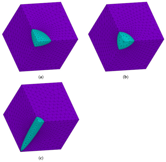
Figure 2. Discretization for one-eighth of the periodic cells using ANSYS (Solid187 element) for different inclusion shapes: (a) discs, (b) spheres and (c) ellipsoids.

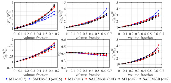
Figure 3. Elastic effective coefficients of two-phase composite (graphite/epoxy) for three different aspect ratios: $\alpha$ = 0.5 (discs), $\alpha$ = 1 (spheres) and $\alpha$ = 2 (ellipsoids). MT: Mori–Tanaka method; SAFEM-3D: three-dimensional semi-analytical finite element method.

The discretization of hollow and massive cylinders is shown in Figure 4. Figure 5 illustrates the behavior of the normalized longitudinal Young’s modulus $(E_{11}^{\ast }/E_{11}^{\left(2\right)})$ for a two-phase FRC (SWNT/LaRC-SI) as a function of the inclusion’s volume fraction. In addition, a comparison between the SAFEM-3D and three different homogenization schemes based on the Mori–Tanaka method (MT) [14] are reported. Here, the SWNT isotropic reinforcement [14] embedded in an isotropic matrix has an aspect ratio of $\alpha =12.3$. The SWNT reinforcement is designed with a hollow cylindrical geometry (see Figure 4a) simulating the carbon nanotube. It can be observed that the SAFEM-3D results are close to those reported by the MT models. Furthermore, there are two types of concavity in the effective behaviors according to different approaches.

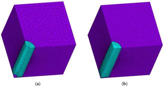
Figure 4. Discretization for one-eighth of the periodic cells using ANSYS (Solid187 element) with (a) hollow and (b) massive cylinders.

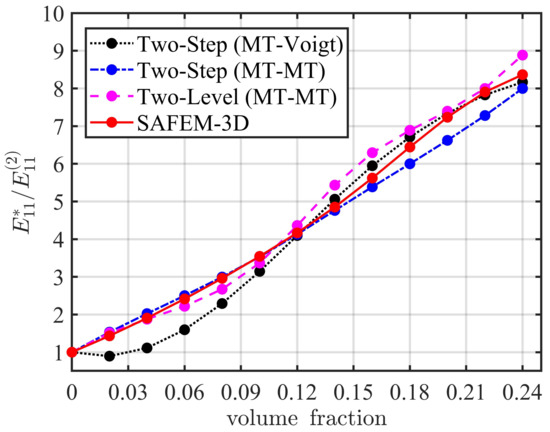
Figure 5. Normalized longitudinal Young’s modulus $(E_{11}^{\ast }/E_{11}^{\left(2\right)})$ as a function of the inclusion’s volume fraction for a two-phase fiber-reinforced composite (FRC) (LaRC-SI/SWNT) with hollow and massive nanotubes in an aligned configuration and aspect ratio of $\alpha =12.3$.

Table 3 shows the effective elastic moduli of a two-phase FRC (Inclusion [46]/matrix [46]) for three different values of the inclusion’s volume fraction: $v_f=0.05$, $v_f=0.2$ and $v_f=0.35$. Here, the constituent properties of the composite are considered as transversely isotropic materials, and cylindrical inclusions (see Figure 4b) are assumed. In addition, a comparison between the analytical AHM and the semi-analytical approaches of SAFEM-2D [46] and SAFEM-3D are reported. An analysis of the relative error is also shown. As can be seen, good agreement between the AHM and the SAFEM-2D is observed. However, a major difference is observed for the SAFEM-3D approach. This is because the SAFEM-3D calculations are developed considering that the fiber’s length in the $y_3$ axial direction is equal to $0.49$ within one-eighth of the cubic cell S with an edge length of $0.5$. Furthermore, it is observed that, as the inclusion volume fraction increases, the relative errors increase, and this is more noticeable for $C_{3333}^{\ast }$. Here, the SAFEM-3D model is an approximation to the long-fiber case. On the other hand, as expected, an increase of the inclusion volume fraction leads to an increment in the effective properties, because the elastic properties of the inclusions are higher than those of the matrix.

Table 3. Effective elastic coefficients (GPa) and relative errors: $\mathrm{Error}1=\left|(C_{\mathbf{AHM}}^{\ast }-C_{\mathbf{SAFEM}-\mathbf{3}\mathbf{D}}^{\ast })/C_{\mathbf{SAFEM}-\mathbf{3}\mathbf{D}}^{\ast }\right|\times 100\%$, $\mathrm{Error}2=\left|(C_{\mathbf{SAFEM}-\mathbf{2}\mathbf{D}}^{\ast }-C_{\mathbf{SAFEM}-\mathbf{3}\mathbf{D}}^{\ast })/C_{\mathbf{SAFEM}-\mathbf{3}\mathbf{D}}^{\ast }\right|\times 100\%$. AHM: asymptotic homogenization method.

${\mathit{C}}_{1111}^{\ast }$
${\mathit{v}}_{\mathit{f}}$	AHM	SAFEM-2D	SAFEM-3D	$\mathrm{Error}1$	$\mathrm{Error}2$
0.05	1.0556	1.0556	1.0555	0.0095	0.0095
0.2	1.2606	1.2607	1.2519	0.6949	0.7029
0.35	1.5436	1.5436	1.5266	1.1136	1.1136
${\mathit{C}}_{\mathbf{1122}}^{\ast }$
${\mathit{v}}_{\mathit{f}}$	AHM	SAFEM-2D	SAFEM-3D	$\mathrm{Error}1$	$\mathrm{Error}2$
0.05	1.0405	1.0445	1.0427	0.2110	0.1726
0.2	1.1565	1.1565	1.2119	4.5713	4.5713
0.35	1.2599	1.2599	1.4511	13.1762	13.1762
${\mathit{C}}_{\mathbf{1133}}^{\ast }$
${\mathit{v}}_{\mathit{f}}$	AHM	SAFEM-2D	SAFEM-3D	$\mathrm{Error}1$	$\mathrm{Error}2$
0.05	1.0223	1.0223	1.0296	0.7090	0.7090
0.2	1.1001	1.1001	1.1269	2.3782	2.3782
0.35	1.2001	1.2001	1.2343	2.7708	2.7708
${\mathit{C}}_{\mathbf{3333}}^{\ast }$
${\mathit{v}}_{\mathit{f}}$	AHM	SAFEM-2D	SAFEM-3D	$\mathrm{Error}1$	$\mathrm{Error}2$
0.05	1.2010	1.2010	1.1526	4.1992	4.1992
0.2	1.8052	1.8052	1.5447	16.8641	16.8641
0.35	2.4119	2.4119	1.9401	24.3183	24.3183
${\mathit{C}}_{\mathbf{1313}}^{\ast }$
${\mathit{v}}_{\mathit{f}}$	AHM	SAFEM-2D	SAFEM-3D	$\mathrm{Error}1$	$\mathrm{Error}2$
0.05	1.0784	1.0784	1.0765	0.1765	0.1765
0.2	1.3555	1.3555	1.3688	0.9717	0.9717
0.35	1.7201	1.7201	1.7633	2.4500	2.4500
${\mathit{C}}_{\mathbf{1212}}^{\ast }$
${\mathit{v}}_{\mathit{f}}$	AHM	SAFEM-2D	SAFEM-3D	$\mathrm{Error}1$	$\mathrm{Error}2$
0.05	1.0625	1.0625	1.0624	0.0094	0.0094
0.2	1.2619	1.2619	1.2788	1.3216	1.3216
0.35	1.5041	1.5041	1.5611	3.6513	3.6513

Table 4 reports the effective elastic moduli of a two-phase FRC computed by a semi-analytical method (SAM) [50], the self-consistent method (SCM) [50] and the SAFEM-3D as a function of the aspect ratios ($\alpha$) and the volume fractions ($v_f$). In addition, an analysis of the relative error between the SAFEM-3D and the other two models (SAM and SCM) is also shown. Here, a two-phase FRC with transversely isotropic ellipsoidal inclusions (Al 6061) embedded in a matrix [50] is assumed; see Table 2. A good agreement among the three models is observed, with a relative error below $1\%$ in every case. This result is to be expected because small inclusion volume fractions are assumed. On the other hand, it is observed that all the effective elastic properties increase as the volume fraction of the ellipsoidal inclusions decreases. This fact is caused by a much stiffer matrix and more matrix material within the system.

Table 4. Effective elastic coefficients (GPa) for a two-phase FRC reinforced by ellipsoidal inclusions with four different aspect ratios ($\alpha$) and volume fractions ($v_f$). Here, the relative errors: $\mathrm{Error}1=\left|(C_{\mathbf{SAM}}^{\ast }-C_{\mathbf{SAFEM}-\mathbf{3}\mathbf{D}}^{\ast })/C_{\mathbf{SAFEM}-\mathbf{3}\mathbf{D}}^{\ast }\right|\times 100\%$ and $\mathrm{Error}2=\left|(C_{\mathbf{SCM}}^{\ast }-C_{\mathbf{SAFEM}-\mathbf{3}\mathbf{D}}^{\ast })/C_{\mathbf{SAFEM}-\mathbf{3}\mathbf{D}}^{\ast }\right|\times 100\%$ are reported.

$\mathit{\alpha }=0.222{\mathit{v}}_{\mathit{f}}=0.085$
${\mathit{C}}_{\mathit{ijkl}}^{\ast }$	SAM	SCM	SAFEM-3D	$\mathbf{Error}\mathbf{1}$	$\mathbf{Error}\mathbf{2}$
$C_{1111}^{\ast }$	2.506	2.499	2.506	0.0000	0.2793
$C_{1122}^{\ast }$	8.097	8.108	8.108	0.1357	0.0000
$C_{1133}^{\ast }$	8.002	8.045	8.002	0.0000	0.5374
$C_{3333}^{\ast }$	2.402	2.402	2.402	0.0000	0.0000
$C_{2323}^{\ast }$	7.949	8.032	7.948	0.0126	1.0569
$C_{1212}^{\ast }$	8.459	8.440	8.458	0.0118	0.2128
$\mathit{\alpha }=\mathbf{0.333}{\mathit{v}}_{\mathit{f}}=\mathbf{0.047}$
${\mathit{C}}_{\mathit{ijkl}}^{\ast }$	SAM	SCM	SAFEM-3D	$\mathbf{Error}\mathbf{1}$	$\mathbf{Error}\mathbf{2}$
$C_{1111}^{\ast }$	2.565	2.563	2.566	0.0390	0.1169
$C_{1122}^{\ast }$	8.220	8.225	8.220	0.0000	0.0608
$C_{1133}^{\ast }$	8.199	8.209	8.209	0.1218	0.0000
$C_{3333}^{\ast }$	2.521	2.517	2.521	0.0000	0.1587
$C_{2323}^{\ast }$	8.524	8.534	8.525	0.0117	0.1056
$C_{1212}^{\ast }$	8.703	8.703	8.707	0.0459	0.0459
$\mathit{\alpha }=\mathbf{0.500}{\mathit{v}}_{\mathit{f}}=\mathbf{0.042}$
${\mathit{C}}_{\mathit{ijkl}}^{\ast }$	SAM	SCM	SAFEM-3D	$\mathbf{Error}\mathbf{1}$	$\mathbf{Error}\mathbf{2}$
$C_{1111}^{\ast }$	2.569	2.568	2.570	0.0389	0.0778
$C_{1122}^{\ast }$	8.241	8.242	8.242	0.0121	0.0000
$C_{1133}^{\ast }$	8.224	8.243	8.224	0.0000	0.2310
$C_{3333}^{\ast }$	2.554	2.542	2.544	0.3931	0.0786
$C_{2323}^{\ast }$	8.621	8.632	8.626	0.0580	0.0696
$C_{1212}^{\ast }$	8.710	8.720	8.720	0.1147	0.0000
$\mathit{\alpha }=\mathbf{0.666}{\mathit{v}}_{\mathit{f}}=\mathbf{0.031}$
${\mathit{C}}_{\mathit{ijkl}}^{\ast }$	SAM	SCM	SAFEM-3D	$\mathbf{Error}\mathbf{1}$	$\mathbf{Error}\mathbf{2}$
$C_{1111}^{\ast }$	2.589	2.587	2.589	0.0000	0.0772
$C_{1122}^{\ast }$	8.279	8.276	8.279	0.0000	0.0362
$C_{1133}^{\ast }$	8.259	8.280	8.280	0.2536	0.0000
$C_{3333}^{\ast }$	2.586	2.575	2.577	0.3492	0.0776
$C_{2323}^{\ast }$	8.748	8.759	8.761	0.1484	0.0228
$C_{1212}^{\ast }$	8.781	8.795	8.799	0.2046	0.0455

Table 5 illustrates the effective elastic coefficients of a three-phase FRC for different volume fractions of the inclusions and computed relative errors ($\mathrm{Error}1$ and $\mathrm{Error}2$), as in Table 4. Here, the composite material is reinforced by ellipsoidal $(\alpha =0.666)$ and spherical $(\alpha =1)$ inclusions. For the computations, the constituents materials of the SiC matrix, spherical inclusions (Al 6061) and ellipsoidal inclusions (matrix [50]) are given in Table 2. In this analysis, the configuration of these inclusions within the composite is performed to validate the SAFEM-3D model within the range aspect ratios and volume fractions used in this work. Additionally, it is worth mentioning that the distribution and shape of the fibers provide a broader view on the scope of the SAFEM-3D model. As can be seen in Table 5, a good agreement is observed between the models. Moreover, the effective elastic properties decrease as the volume fraction of both inclusions increase. This fact is due to a stiffer SiC matrix being considered; therefore, there is less matrix material in the system. Here, the relative errors are in general below $2.2\%$.

Table 5. Effective elastic coefficients (GPa) for a three-phase FRC reinforced by ellipsoidal and spherical inclusions for different aspect ratios ($\alpha$) and volume fractions ($v_f$).

$\mathit{\alpha }=0.666{\mathit{v}}_{\mathit{f}}=0.023\mathit{\alpha }=1.000{\mathit{v}}_{\mathit{f}}=0.035$
${\mathit{C}}_{\mathit{ijkl}}^{\ast }$	SAM	SCM	SAFEM-3D	$\mathbf{Error}\mathbf{1}$	$\mathbf{Error}\mathbf{2}$
$C_{1111}^{\ast }$	4.492	4.519	4.484	0.1784	0.7806
$C_{1122}^{\ast }$	9.782	9.686	9.700	0.8454	0.1443
$C_{1133}^{\ast }$	9.654	9.713	9.650	0.0415	0.6528
$C_{3333}^{\ast }$	4.496	4.483	4.477	0.4244	0.1340
$C_{2323}^{\ast }$	1.748	1.764	1.750	0.1143	0.8000
$C_{1212}^{\ast }$	1.765	1.775	1.761	0.2271	0.7950
$\mathit{\alpha }=\mathbf{0.666}{\mathit{v}}_{\mathit{f}}=\mathbf{0.026}\mathit{\alpha }=\mathbf{1.000}{\mathit{v}}_{\mathit{f}}=\mathbf{0.043}$
${\mathit{C}}_{\mathit{ijkl}}^{\ast }$	SAM	SCM	SAFEM-3D	$\mathbf{Error}\mathbf{1}$	$\mathbf{Error}\mathbf{2}$
$C_{1111}^{\ast }$	4.436	4.468	4.426	0.2259	0.9489
$C_{1122}^{\ast }$	9.780	9.658	9.678	1.0539	0.2067
$C_{1133}^{\ast }$	9.621	9.690	9.605	0.1666	0.8850
$C_{3333}^{\ast }$	4.438	4.424	4.417	0.4754	0.1585
$C_{2323}^{\ast }$	1.719	1.737	1.719	0.0000	1.0471
$C_{1212}^{\ast }$	1.741	1.751	1.734	0.4037	0.9804
$\mathit{\alpha }=\mathbf{0.666}{\mathit{v}}_{\mathit{f}}=\mathbf{0.036}\mathit{\alpha }=\mathbf{1.000}{\mathit{v}}_{\mathit{f}}=\mathbf{0.055}$
${\mathit{C}}_{\mathit{ijkl}}^{\ast }$	SAM	SCM	SAFEM-3D	$\mathbf{Error}\mathbf{1}$	$\mathbf{Error}\mathbf{2}$
$C_{1111}^{\ast }$	4.360	4.396	4.346	0.3221	1.1505
$C_{1122}^{\ast }$	9.778	9.619	9.644	1.3895	0.2592
$C_{1133}^{\ast }$	9.572	9.658	9.536	0.3775	1.2794
$C_{3333}^{\ast }$	4.358	4.342	4.334	0.5538	0.1846
$C_{2323}^{\ast }$	1.678	1.700	1.675	0.1791	1.4925
$C_{1212}^{\ast }$	1.709	1.717	1.698	0.6478	1.1190
$\mathit{\alpha }=\mathbf{0.666}{\mathit{v}}_{\mathit{f}}=\mathbf{0.048}\mathit{\alpha }=\mathbf{1.000}{\mathit{v}}_{\mathit{f}}=\mathbf{0.075}$
${\mathit{C}}_{\mathit{ijkl}}^{\ast }$	SAM	SCM	SAFEM-3D	$\mathbf{Error}\mathbf{1}$	$\mathbf{Error}\mathbf{2}$
$C_{1111}^{\ast }$	4.253	4.293	4.231	0.5200	1.4654
$C_{1122}^{\ast }$	9.775	9.561	9.593	1.8972	0.3336
$C_{1133}^{\ast }$	9.495	9.608	9.426	0.7320	1.9308
$C_{3333}^{\ast }$	4.243	4.224	4.213	0.7121	0.2611
$C_{2323}^{\ast }$	1.620	1.646	1.611	0.5587	2.1726
$C_{1212}^{\ast }$	1.665	1.668	1.646	1.1543	1.3366

Figure 6 illustrates the longitudinal Young’s modulus $\left(E_{11}^{\ast }\right)$ as a function of the nanotube length, for a two-phase composite reinforced by aligned isotropic SWNT nanotubes [12] in a LaRC-SI polymeric matrix. Here, the SWNT nanotubes are simulated by ellipsoidal inclusions within a matrix. In addition, a comparison between the SAFEM-3D and the continuous-equivalent method [12] is reported. The numerical calculations are performed considering a SWNT nanotube volume fraction equal to 0.01. As can be seen, very good agreement is observed.

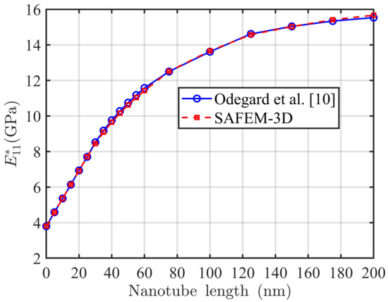
Figure 6. Effective longitudinal Young’s modulus for a two-phase FRC with an aligned isotropic SWNT nanotube [12] with a $1\%$ volume fraction.

4.2. Random NTC Reinforced Composites

In this section, the effect of the distribution of inclusions on the effective longitudinal Young’s modulus $\left(E_{11}^{\ast }\right)$ property is studied. For this purpose, the SAFEM-3D is implemented over different two-phase FRCs, in which the periodic unit cell has 72 similar inclusions embedded in the matrix. The effect of non-aligned inclusions is determined by their rotations with respect to the axial axis $y_1$. Different fiber orientations $(\theta =0^{\circ }\left(\mathrm{aligned}\mathrm{inclusions}\right),{10}^{\circ },{15}^{\circ },{20}^{\circ },{25}^{\circ },{30}^{\circ },\mathrm{and}{35}^{\circ }\left(\mathrm{random}\mathrm{inclusions}\right))$ are considered. Non-alignment is implemented by dividing one-eighth of the cell into nine prisms containing a single inclusion, which are assumed to have different orientations. No contact between inclusions is allowed. Then, the inclusions are randomly oriented around the axial axis, but all of them have a fixed angle with respect to that axis. In this way, the effect of non-aligned inclusions can be described. For transversely isotropic inclusions, the elastic tensor should be rotated according to the inclusion orientation. In Figure 7, the discretization for one-eighth of the periodic cells using ANSYS (solid187 element) is shown for different inclusion shapes (discs, spheres and ellipsoids) with $1\%$ of the inclusion volume fraction.

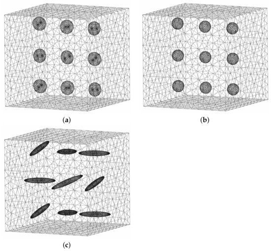
Figure 7. Discretization for one-eighth of the periodic cells using ANSYS (Solid187 element) for different inclusion shapes with a $1\%$ inclusion volume fraction and a ${10}^{\circ }$ fiber orientation: (a) discs ($\alpha =0.6$), (b) spheres ($\alpha =1$) and (c) ellipsoids ($\alpha =10$).

In Figure 8, the effective longitudinal Young’s modulus $\left(E_{11}^{\ast }\right)$ as a function of the inclusion aspect ratio $\alpha$ is shown for a two-phase FRC with aligned ($\theta =0^{\circ }$) and random ($\theta ={35}^{\circ }$) transversely isotropic SWNT [13] inclusions in an isotropic LaRC-SI matrix. Here, the numerical calculation is determined considering a $1\%$ SWNT volume fraction for different aspect ratio values $0\le \alpha \le 14$. The inclusion shapes for $\alpha =0.6,1\mathrm{and}10$ can be seen in Figure 7. Additionally, a comparison between the SAFEM-3D and the deformation energy method based on the Mori–Tanaka model [12,13] is reported. A good agreement is observed between both models. From Figure 8, it is observed that the aligned nanotubes array shows a maximum value of the longitudinal Young’s modulus in the whole range of aspect ratio values.

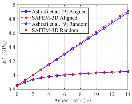
Figure 8. Longitudinal Young’s modulus for fibers in aligned and random configurations for a 1% SWNT/LaRC-SI composite.

In Figure 9, the effective longitudinal Young’s modulus $\left(E_{11}^{\ast }\right)$ as a function of the inclusion’s aspect ratio $\alpha$ for different fiber orientations $(\theta =0^{\circ }\left(\mathrm{aligned}\right),{10}^{\circ },{15}^{\circ },{20}^{\circ },{25}^{\circ },{30}^{\circ },\mathrm{and}{35}^{\circ }\left(\mathrm{random}\right))$ is shown. Here, the periodic FRC is defined by transversely isotropic SWNT [13] inclusions (see Figure 7) in an isotropic LaRC-SI matrix, where a $1\%$ SWNT volume fraction is considered. Besides, a comparison between the SAFEM-3D and the deformation energy method based on the Mori–Tanaka model [12,13] is given for aligned and random fiber distributions. The comparisons show good agreement. From Figure 9, it is observed that the effective longitudinal Young’s modulus $\left(E_{11}^{\ast }\right)$ has a strong dependence on the fiber orientation. As $\theta$ increases, the value of the longitudinal Young’s modulus decreases. Maximum values of $E_{11}^{\ast }$ are obtained for the aligned distribution of the inclusions.

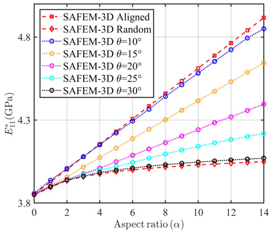
Figure 9. Effective longitudinal Young’s modulus $\left(E_{11}^{\ast }\right)$ as a function of the inclusion’s aspect ratio $\alpha$ for a composite with different fiber orientations and $1\%$ SWNT volume fraction.

The effect of carbon nanowire (CNW) inclusions on the effective longitudinal Young’s modulus $\left(E_{11}^{\ast }\right)$ is now presented. The CNWs are simulated by ellipsoidal inclusions with different orientations, as seen in Figure 10. In Figure 11, the behavior of $E_{11}^{\ast }$ as a function of the CNW weight content (CNW wt content)$(\%)$ for different CNW orientations $\theta =0^{\circ }\left(\mathrm{Aligned}\right),{10}^{\circ },{20}^{\circ },{30}^{\circ }\mathrm{and}{35}^{\circ }\left(\mathrm{Random}\right)$ is reported. In addition, a comparison between the SAFEM-3D results and experimental data [10] is shown. For the numerical computation, the material constituents of the matrix (polystyrene) and the CNW inclusions are assumed to be isotropic materials, such as $E=3.349$ GPa and $\nu =0.34$ for polystyrene [10] and $E=169$ GPa and $\nu =0.185$ for CNW [51]. As can be observed, the theoretical results using the SAFEM-3D show that $E_{11}^{\ast }$ decreases as $\theta$ increases; i.e., $E_{11}^{\ast }$ for aligned CNW inclusions ($\theta =0$) is greater than that for random CNW inclusions ($\theta ={35}^{\circ }$) in the $y_1$ axial direction. It is remarkable that the SAFEM-3D values for random inclusions are within the expected error range when the CNW inclusions are between $1\%$ and $5\%$ CNW wt content. From a physical point of view, as the CNT wt content increases, $E_{11}^{\ast }$ should grow, as can be seen in the SAFEM-3D results (Figure 11). The difference between the SAFEM-3D values and the experimental values when the CNW inclusions have $5\%$ CNW wt content is also reported in [10].

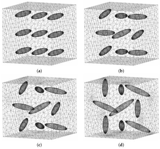
Figure 10. Periodic unit cell mesh for different fiber orientations (a) $\theta =0^{\circ }\left(\mathrm{aligned}\mathrm{inclusions}\right)$, (b) $\theta ={10}^{\circ }$, (c) $\theta ={20}^{\circ }$ and (d) $\theta ={35}^{\circ }\left(\mathrm{random}\mathrm{inclusions}\right))$.

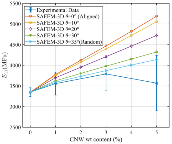
Figure 11. Effective longitudinal Young’s modulus $\left(E_{11}^{\ast }\right)$ as a function of the carbon nanowire (CNW) weight content$(\%)$. A comparison between the SAFEM-3D results and experimental data is shown.

5. Conclusions

In this work, the estimation of the effective elastic properties of periodic reinforced nanocomposites is developed. The nanocomposites are defined with isotropic or transversely isotropic inclusions embedded in an isotropic matrix. Different inclusions in the form of discs, ellipsoidals, spheres, carbon nanotubes and carbon nanowires are also considered. Two configurations of inclusions are taken into account: aligned and random. A three-dimensional semi-analytical approach (SAFEM-3D) is implemented, using a combination of the asymptotic homogenization method and the finite element method. The asymptotic homogenization method provides the local problems and the effective coefficients, whereas the finite element method gives the solution to the local problem by using the minimum potential energy.

The results have been compared with theoretical models validating the efficiency and accuracy of the SAFEM-3D for the analysis of the composites. Based on the numerical results, we have concluded that fiber-reinforced composites with aligned nanotube inclusions show a higher effective longitudinal Young’s modulus than random nanotube arrays. Random carbon nanotube arrays show that the nanotube length has a significant effect on the composite elastic properties in the axial direction. Furthermore, according to the values of the computed relative errors , it is concluded that the SAFEM-3D values have a relative error less than 2.2% when compared with the other reported theoretical models; see Table 4 and Table 5. These results show the efficiency and accuracy of the SAFEM-3D model. For the case of long fibers, a slight difference is observed between SAFEM-3D and AHM (or SAFEM-2D) values when the inclusion volume fraction increases; see Table 3. This error increment is not attributed to the accuracy of SAFEM-3D; it is rather a result of the fact that the long fibers are not considered in the model.

A comparison with experimental data for CNW nanocomposites is reported and a good agreement is obtained. An increase in the CNW weight content enhances the magnitude of $E_{11}^{\ast }$. This effect is described by the SAFEM-3D results for different orientations of inclusions. This is also observed in the experiment when the CNW weight content is $1\%$ and $3\%$; however, when the CNW weight content is equal to $5\%$, a decrease in the property is observed. From the physical point of view, we consider that this last result is not consistent with the expected behavior; thus, we assume that it is a consequence of the composite’s manufacture.

An important advantage of the SAFEM-3D approach is the possibility to design any kind of geometry reinforcement for any type of material, including isotropic and transversely isotropic nanocomposites in three-dimensional configurations for a huge range of random angle values.

References

- Kausar, A.; Rafique, I.; Muhammad, B. Review of applications of polymer/carbon nanotubes and epoxy/CNT composites. Polym. Plast. Technol. Eng. 2016, 55, 1167–1191. [Google Scholar] [CrossRef]
- Fujisawa, K.; Kim, H.J.; Go, S.H.; Muramatsu, H.; Hayashi, T.; Endo, M.; Hirschmann, T.C.; Dresselhaus, M.S.; Kim, Y.A.; Araujo, P.T. A Review of Double-Walled and Triple-Walled Carbon Nanotube Synthesis and Applications. Appl. Sci. 2016, 6, 109. [Google Scholar] [CrossRef]
- Kausar, A.; Rafique, I.; Muhammad, B. Aerospace application of polymer nanocomposite with carbon nanotube, graphite, graphene oxide, and nanoclay. Polym. Plast. Technol. Eng. 2017, 56, 1438–1456. [Google Scholar] [CrossRef]
- Elmarakbi, A.; Karagiannidis, P.; Ciappa, A.; Innocente, F.; Galise, F.; Martorana, B.; Bertocchi, F.; Cristiano, F.; Villaro, E.; Gomez, J. 3-Phase hierarchical graphene-based epoxy nanocomposite laminates for automotive applications. J. Mater. Sci. Technol. 2019, 35, 2169–2177. [Google Scholar] [CrossRef]
- Oraon, R.; De Adhikari, A.; Tiwari, S.K.; Nayak, G.C. Enhanced specific capacitance of self-assembled three-dimensional carbon nanotube/layered silicate/polyaniline hybrid sandwiched nanocomposite for supercapacitor applications. ACS Sustain. Chem. Eng. 2016, 4, 1392–1403. [Google Scholar] [CrossRef]
- Kinloch, I.A.; Suhr, J.; Lou, J.; Young, R.J.; Ajayan, P.M. Composites with carbon nanotubes and graphene: An outlook. Science 2018, 362, 547–553. [Google Scholar] [CrossRef]
- DeGraff, J.; Liang, R.; Le, M.Q.; Capsal, J.F.; Ganet, F.; Cottinet, P.J. Printable low-cost and flexible carbon nanotube buckypaper motion sensors. Mater. Des. 2017, 133, 47–53. [Google Scholar] [CrossRef]
- Kim, J.H.; Hwang, J.Y.; Hwang, H.; Kim, H.S.; Lee, J.H.; Seo, J.W.; Shin, U.S.; Lee, S.H. Simple and cost-effective method of highly conductive and elastic carbon nanotube/polydimethylsiloxane composite for wearable electronics. Sci. Rep. 2018, 8, 1–11. [Google Scholar] [CrossRef]
- Go, M.-S.; Park, S.-M.; Kim, D.-W.; Hwang, D.-S.; Lim, J.H. Random Fiber Array Generation Considering Actual Noncircular Fibers with a Particle-Shape Library. Appl. Sci. 2020, 10, 5675. [Google Scholar] [CrossRef]
- Kostas, V.; Baikousi, M.; Barkoula, N.-M.; Giannakas, A.; Kouloumpis, A.; Avgeropoulos, A.; Gournis, D.; Karakassides, M.A. Synthesis, Characterization and Mechanical Properties of Nanocomposites Based on Novel Carbon Nanowires and Polystyrene. Appl. Sci. 2020, 10, 5737. [Google Scholar] [CrossRef]
- Weng, G.J. Some elastic properties of reinforced solids, with special reference to isotropic ones containing spherical inclusions. Int. J. Eng. Sci. 1984, 22, 845–856. [Google Scholar] [CrossRef]
- Odegard, G.M.; Gates, T.S.; Wise, K.E.; Park, C.; Siochi, E.J. Constitutive modeling of nanotube–reinforced polymer composites. Compos. Sci. Technol. 2003, 63, 1671–1687. [Google Scholar] [CrossRef]
- Ashrafi, B.; Hubert, P. Modeling the elastic properties of carbon nanotube array/polymer composites. Compos. Sci. Technol. 2006, 66, 387–396. [Google Scholar] [CrossRef]
- Selmi, A.; Friebel, C.; Doghri, I.; Hassis, H. Prediction of the elastic properties of single walled carbon nanotube reinforced polymers: A comparative study of several micromechanical models. Compos. Sci. Technol. 2007, 67, 2071–2084. [Google Scholar] [CrossRef]
- Guinovart-Díaz, R.; Rodríguez-Ramos, R.; Bravo-Castillero, J.; Sabina, F.J.; Otero- Hernández, J.A.; Maugin, G.A. A recursive asymptotic homogenization scheme for multi-phase fibrous elastic composites. Mech. Mater. 2005, 37, 1119–1131. [Google Scholar] [CrossRef]
- Hadjiloizi, D.A.; Georgiades, A.V.; Kalamkarov, A.L. Dynamic modeling and determination of effective properties of smart composite plates with rapidly varying thickness. Int. J. Eng. Sci. 2012, 56, 63–85. [Google Scholar] [CrossRef]
- Bakhvalov, N.S.; Panasenko, G.P. Homogenisation: Averaging Processes in Periodic Media; (Soviet Series); Kluwer Academic Publishers Group: Dordrecht, The Netherlands, 1989. [Google Scholar]
- Challagulla, K.S.; Georgiades, A.V.; Kalamkarov, A.L. Asymptotic homogenization modeling of smart composite generally orthotropic grid-reinforced shells: Part I–theory. Eur. J. Mech. A Solids 2010, 29, 530–540. [Google Scholar] [CrossRef]
- Berger, H.; Kari, S.; Gabbert, U.; Rodríguez-Ramos, R.; Bravo-Castillero, J.; Guinovart-Díaz, R. Calculation of effective coefficients for piezoelectric fiber composites based on a general numerical homogenization technique. Compos. Struct. 2005, 71, 397–400. [Google Scholar] [CrossRef]
- Kalamkarov, A.L.; Andrianov, I.V.; Danishevs’kyy, V.V. Asymptotic homogenization of composite materials and structures. Appl. Mech. Rev. 2009, 62, 030802. [Google Scholar] [CrossRef]
- Pal, G.; Kumar, S. Modeling of carbon nanotubes and carbon nanotube–polymer composites. Prog. Aerosp. Sci. 2016, 80, 33–58. [Google Scholar] [CrossRef]
- Bravo-Castillero, J.; Rodríguez-Ramos, R.; Mechkour, H.; Otero, J.A.; Hernández-Cabanas, J.; Sixto, L.M.; Guinovart-Díaz, R.; Sabina, F.J. Homogenization and effective properties of periodic thermomagnetoelectroelastic composites. J. Mech. Mater. Struct. 2009, 4, 819–836. [Google Scholar] [CrossRef]
- Rodríguez-Ramos, R.; Berger, H.; Guinovart-Díaz, R.; López-Realpozo, J.C.; Würkner, M.; Gabbert, U.; Bravo-Castillero, J. Two approaches for the evaluation of the effective properties of elastic composite with parallelogram periodic cells. Int. J. Eng. Sci. 2012, 58, 2–10. [Google Scholar] [CrossRef]
- Zhao, J.; Li, H.; Cheng, G.; Cai, Y. On predicting the effective elastic properties of polymer nanocomposites by novel numerical implementation of asymptotic homogenization method. Compos. Struct. 2016, 135, 297–305. [Google Scholar] [CrossRef]
- Baek, K.; Shin, H.; Yoo, T.; Cho, M. Two-step multiscale homogenization for mechanical behaviour of polymeric nanocomposites with nanoparticulate agglomerations. Compos. Sci. Technol. 2019, 179, 97–105. [Google Scholar] [CrossRef]
- Rossi, M.; Meo, M. On the estimation of mechanical properties of single-walled carbon nanotubes by using a molecular-mechanics based FE approach. Compos. Sci. Technol. 2009, 69, 1394–1398. [Google Scholar] [CrossRef]
- Cheng, G.-D.; Cai, Y.-W.; Xu, L. Novel implementation of homogenization method to predict effective properties of periodic materials. Acta Mech. Sin. 2013, 29, 550–556. [Google Scholar] [CrossRef]
- Kassa, M.K.; Arumugam, A.B. Micromechanical modeling and characterization of elastic behavior of carbon nanotube-reinforced polymer nanocomposites: A combined numerical approach and experimental verification. Polym. Compos. 2020, 41, 3322–3339. [Google Scholar] [CrossRef]
- Otero, J.A.; Rodríguez-Ramos, R.; Monsivais, G. Computation of effective properties in elastic composites under imperfect contact with different inclusion shapes. Math. Meth. Appl. Sci. 2016, 40, 3290–3310. [Google Scholar] [CrossRef]
- Espinosa-Almeyda, Y.; Camacho-Montes, H.; Otero, J.A.; Rodríguez-Ramos, R.; López-Realpozo, J.C.; Guinovart-Díaz, R.; Sabina, F.J. Interphase effect on the effective magneto-electro-elastic properties for three-phase fiber-reinforced composites by a semi-analytical approach. Int. J. Eng. Sci. 2020, 154, 103310. [Google Scholar] [CrossRef]
- Gabbert, U.; Kari, S.; Bohn, N.; Berge, H. Numerical homogenization and optimization of smart composite materials. In Mechanics and Model-Based Control of Smart Materials and Structures; Irschik, H., Ed.; Springer: Vienna, Austria, 2010; pp. 59–68. [Google Scholar]
- Nasution, M.R.E.; Watanabe, N.; Kondo, A.; Yudhanto, A. A novel asymptotic expansion homogenization analysis for 3-D composite with relieved periodicity in the thickness direction. Compos. Sci. Technol. 2014, 97, 63–73. [Google Scholar] [CrossRef]
- Pike, M.G.; Oskay, C. Three-Dimensional Modeling of Short Fiber-Reinforced Composites with Extended Finite-Element Method. J. Eng. Mech. 2016, 142, 1–12. [Google Scholar] [CrossRef]
- Fisher, F.T.; Bradshaw, R.D.; Brinson, L.C. Effects of nanotube waviness on the modulus of nanotube-reinforced polymers. Appl. Phys. Lett. 2002, 80, 4647–4649. [Google Scholar] [CrossRef]
- Fisher, F.T.; Bradshaw, R.D.; Brinson, L.C. Fiber waviness in nanotube–reinforced polymer composites—I: Modulus predictions using effective nanotube properties. Compos. Sci. Technol. 2003, 63, 1689–1703. [Google Scholar] [CrossRef]
- Thakur, A.K.; Kumar, P.; Srinivas, J. Studies on Effective Elastic Properties of CNT/Nano-Clay Reinforced Polymer Hybrid Composite. IOP Conf. Ser. Mater. Sci. Eng. 2016, 115, 12007. [Google Scholar] [CrossRef]
- David Müzel, S.; Bonhin, E.P.; Guimarães, N.M.; Guidi, E.S. Application of the Finite Element Method in the Analysis of Composite Materials: A Review. Polymers 2020, 12, 818. [Google Scholar] [CrossRef]
- Tarfaoui, M.; Lafdi, K.; El Moumen, A. Mechanical properties of carbon nanotubes based polymer composites. Compos. Part B Eng. 2016, 103, 113–121. [Google Scholar] [CrossRef]
- Choi, J.; Shin, H.; Cho, M. A multiscale mechanical model for the effective interphase of SWNT/epoxy nanocomposite. Polymer 2016, 89, 159–171. [Google Scholar] [CrossRef]
- El Moumen, A.; Tarfaoui, M.; Lafdi, K. Computational Homogenization of Mechanical Properties for Laminate Composites Reinforced with Thin Film Made of Carbon Nanotubes. Appl. Compos. Mater. 2017, 25, 569–588. [Google Scholar] [CrossRef]
- Yengejeh, S.I.; Kazemi, S.A.; Öchsner, A. Carbon nanotubes as reinforcement in composites: A review of the analytical, numerical and experimental approaches. Comput. Mater. Sci. 2017, 136, 85–101. [Google Scholar] [CrossRef]
- Saad, M.H. Elasticity: Theory, Applications, and Numerics; Elsevier: Burlington, MA, USA; Butterworth Heinemann: Oxford, UK, 2005. [Google Scholar]
- Landau, L.D.; Lifshits, E.M. Theory of Elasticity, 2nd ed.; Pergamon Press Inc.: New York, NY, USA, 1970. [Google Scholar]
- Bensoussan, A.; Lions, J.L.; Papanicolaou, G. Asymptotic Analysis for Periodic Structures; North-Holland: New York, NY, USA, 1978. [Google Scholar]
- Sanchez-Palencia, E. Non-Homogeneous Media and Vibration Theory; Lecture Notes in Physics, 127; Springer: Berlin, Germany, 1980. [Google Scholar]
- Otero, J.A.; Rodríguez-Ramos, R.; Bravo-Castillero, J.; Guinovart-Díaz, R.; Sabina, F.J.; Monsivais, G. Semi-analytical method for computing effective properties in elastic composite under imperfect contact. Int. J. Solids Struct. 2013, 50, 609–622. [Google Scholar] [CrossRef]
- Chandrupatla, T.R.; Belegundu, A.D. Introduction to Finite Elements in Engineering, 3rd ed.; Prentice Hall: Upper Saddle River, NJ, USA, 2002; pp. 13–102. [Google Scholar]
- Zienkiewicz, O.C.; Taylor, R.L.; Zhu, J.Z. The Finite Element Method: Its Basis and Fundamentals, 7th ed.; Butterworth-Heinemann: Oxford, UK, 2013. [Google Scholar]
- Dvorak, G.J. Micromechanics of Composite Materials, 1st ed.; Springer: Dordrecht, The Netherlands, 2013. [Google Scholar]
- Sabina, F.J.; Gandarrilla-Pérez, C.A.; Otero, J.A.; Rodríguez-Ramos, R.; Bravo-Castillero, J.; Guinovart-Díaz, R.; Valdiviezo-Mijangos, O. Dynamic homogenization for composites with embedded multioriented ellipsoidal inclusions. Int. J. Solids Struct. 2015, 69, 121–130. [Google Scholar] [CrossRef]
- Sohn, Y.-S.; Park, J.; Yoon, G.; Song, J.; Jee, S.-W.; Lee, J.-H.; Na, S.; Kwon, T.; Eom, K. Mechanical Properties of Silicon Nanowires. Nanoscale Res. Lett. 2010, 5, 211–216. [Google Scholar] [CrossRef]
Publisher’s Note: MDPI stays neutral with regard to jurisdictional claims in published maps and institutional affiliations. |
© 2021 by the authors. Licensee MDPI, Basel, Switzerland. This article is an open access article distributed under the terms and conditions of the Creative Commons Attribution (CC BY) license (http://creativecommons.org/licenses/by/4.0/).