CFD Analysis of a Tubular Heat Exchanger for the Conditioning of Olive Paste

Abstract

The use of a heat exchanger for the conditioning of the olive paste could enhance the olive oil extraction process. Particularly, paste pre-heating could reduce the malaxation time and, most of all, improve the temperature control during this process (e.g., 27 °C). In this study, a three-dimensional computational fluid dynamics (CFD) analysis of a tubular heat exchanger was carried out to better understand the influence of the inlet conditions of the olive paste on thermal and hydrodynamic behavior within it. CFD analysis was performed with SOLIDWORKS Flow Simulation (ver.2016). The heat exchanger consists of a tube-in-tube module, in which the inner tube was fed with the olive paste, while the jacket was filled of hot water. The main aim was that to predict the heat transfer and pressure drop in paste side of the exchanger. Multiple analyses by varying the mass flow rate and inlet temperature of the paste were carried out, and temperature and pressure drop were estimated. The numerical model has proved very useful in identifying the main factors affecting the optimization of the heat exchanger in order to improve the extraction process of the olive paste.

1. Introduction

Heat exchangers are thermodynamic equipment widely used in food processing industries mainly for different type of engineering applications such as heating and cooling as reported in [1,2,3].

Just as in many food industries also in the industry of extracting virgin oil from olives, there is the need to thermally adapt the olive pastes during the process. The olive pastes temperature adjustment is carried out by the malaxer machine during the malaxation phase. The malaxation process is performed in a machine that consists of a stainless steel chamber with a cradle or circular section, having in its inside a horizontal shaft mounting a series of stainless steel blades to slow mixing the olive paste [4]. The olive paste traditionally is loaded in the malaxer machine and heated to 24–27 °C for up to 30–45 min. The previously reported malaxation time/temperature ranges are recognized by the academic community as optimal to ensure high olive oil quality at the end of the process. In [5], a temperature of 25 °C and times ranging between 30 and 45 min were the optimal operative conditions for the malaxation to optimize sensory characteristics, secoiridoid compounds and the volatile composition of oils extracted from olive fruits from Coratna and Frantoio cultivars. In [6], the optimal malaxation time/temperature was identified in 30 min at 26 °C to preserve the volatile and phenolic composition of the olive oil from olives of Moraiolo cultivar.

The heating of the olive paste is achieved through energy exchanges with a service fluid (hot water) that flows through an external coil [4,7,8]. During malaxation, due to the discontinuity of operation of the machine and due to the inadequate ratio between the heat exchange surface and the volume of the processed product, various negative aspects that significantly affect the functionality of the plant and the quality of the final oil occur. These aspects are reported in [9] such as: (i) time and temperature profiles of the olive paste that depend on the filling levels of the malaxer; (ii) time and temperature profile is not uniform for all olive paste particles in the malaxer due to a small portion of olive paste that can remain attached to the walls of the malaxer through many subsequent cycles; (iii) long operating times, in fact, the malaxation process consumes approximately two-thirds of the total time required for extra-virgin olive oil processing.

In recent years, enormous efforts are being made in terms of energy saving in the food industry sector [10,11]. As regards the mechanical extraction process of virgin olive oil (VOO), important lines of research have been focused on the introduction of new technologies to overcome the negative aspects that occur during the malaxation phase and consequently improve the production and quality of VOO. Various technological innovations in the VOO industry have been studied, such as microwave-assisted systems, low-frequency ultrasound, high-frequency ultrasound and pulsed electric fields, to obtain a positive impact on the extractability of the decanter, on the continuity of the process and, in several cases, on the quality of the olive oil [9,12,13,14,15].

An important innovation introduced in recent years in the mill to significantly reduce the time required to reach the optimal temperature of the olive pastes was the heat exchanger.

First research regarding the application of heat exchange in the olive oil extraction process was carried out by [16], introducing a spiral heat exchanger between the crusher and malaxer, which proved to have a positive influence on the improvement of the malaxation efficiency because of the increment of olive oil extraction yield and the significant improvement in olive oil quality. However, due to clogging and cleaning problems at the end of the process related to the spiral heat exchanger, new technologies such as the tube-in-tube heat exchanger have been tested and subsequently implemented, albeit sparingly, in industrial oil extraction plants.

Recently, several authors [17,18] studied the use of tubular heat exchangers experimentally during the olive oil extraction process, to assess its influence on the processing time, olive oil extraction yield and the quality of the olive oil. These studies proved a significant improvement in the olive oil aromatic fraction and the relative EVOO quality. As well, they confirm the possibility of using a heat exchanger to rapidly increase the olive paste temperature before malaxation and the possibility of reducing the olive paste conditioning time. Research conducted by [19] by using the tube-in-tube heat exchanger between crusher and the malaxer machine on the industrial scale demonstrated that the malaxation time can be reduced to 10 min without any reduction in phenolic content (357.9 g/kg). When the malaxation time, after the flash heating treatment, was risen to 30 min, the phenol content was increased by 17% when the olives were milled with a disc crusher and 27% with a de-pitting machine. While the oil extraction yield is statistically equal to the traditional process yield when the heat exchanger was employed. A recent technology introduced in the mechanical extraction process of olive oil is reported in [20], where a cooling treatment of the olive paste (from 30 to 25 °C) before malaxation step was performed by using a tube-in-tube heat exchanger. The results showed that the cooling treatment leads to a significant improvement of phenolic compounds in the oils. In addition, by malaxing at 30 °C compared to 25 °C, for the same time, no difference in oil yield was found.

An innovative heat exchanger was employed in a commercial olive oil extraction plant by [21], which is the mixing-coil heat exchanger, having a mixing-coil inside. The research demonstrated that the mixing-coil heat exchanger completed the malaxer, and malaxation time was reduced of about 50% compared to the time used in the traditional malaxing without heat exchanger. Similarly, the research reported by [22], which consists of a combination of industrial olive oil extraction plant with a spiral heat exchanger and other advanced technologies, demonstrated that using a heat exchanger in addition to the malaxer generates rapid heating of the olive paste and, therefore, reduced the conditioning time of about 20 min.

In the tube-in-tube heat exchanger, the product to be heated/cooled flows in the inner cylinder, while the service fluid in the annular section between the two cylinders and the heat exchange between the heat transfer fluids occurs under transient state operation through a conductive element, which allows the management of the heat or cold demand in the heat exchanger. However, when the fluid passing through the exchanger is highly viscous or is a sticky fluid such as olive pastes the convective heat transfer mechanism generates critical conditions due to the limited heat transfer coefficients that can be achieved given the low Reynolds number values that generally characterize the fluid flow [23].

In the olive oil industry, olives have a variable inlet temperature during harvesting period and during the 24 h of processing. The olives in fact, before processing, stop in outdoor spaces of the mills; therefore, their inlet temperature is strongly dependent on the environmental one. This causes, for the same setting of the feed pump, a different flow rate of the pastes in the heat exchanger and, consequently, a different heat exchange effect. In addition, although the tube-in-tube heat exchanger is a well-known technology and used in many food industries, its application and behavior on olive pastes is not well known, despite the increasing use of this technology in industrial mills.

To this purpose, mathematical modelling could represent a powerful tool for understanding the performance of a heat exchanger in heat transfer when some parameters change. As it is known, CFD analysis is essential to optimize the design of component without realizing expensive prototypes and experimental tests. CFD applications in food processing are manifold. In [4], the authors developed a 3D CFD simulation model for two different geometry configurations of the malaxer machine to evaluate the design parameter’s influence on the flow and temperature fields. In [23], a scraped surface heat exchanger (SSHE) with alternate blades to heat hazelnut paste was analyzed by means of three-dimensional axial-symmetric CFD simulation. [24] modelled the flow and heat transfer in an SSHE during the production of sorbet to analyze the 3D distributions of the main variables and to assess the performance of this model under different operating conditions. CFD analysis was also used for complex phenomena, such as the leaf paradox phenomena in a whirlpool for solid separation in the brewing industry [25].

The main objective of this scientific research is to carry out a theoretical study aimed at evaluating the behavior of a well-known technology (tube-in-tube heat exchanger) in a new industrial application, namely the olive oil extraction process.

In this research, a three-dimensional CFD analysis was performed to predict the heat transfer behavior and pressure drop in a tube-in-tube heat exchanger, when the mass flow rate and inlet temperature of the olive paste varied according to typical operative conditions.

This article represents a theoretical study on the applicability of the tube-in-tube heat exchanger for the conditioning of olive pastes to obtain valuable information on its application and behavior, in order to improve its use in industrial plants for the extraction of olive oil.

2. Materials and Methods

In this study, the CFD analysis was performed by SOLIDWORKS Flow Simulation. It is worth noting that other research has utilized SOLIDWORKS Flow Simulation in similar and more severe flow conditions with considerable accuracy [26,27,28,29,30].

2.1. Physical Model of the Studied Heat Exchanger

The studied heat exchanger consists of an inner tube and external jacket. In the inner tube flows the olive paste, which must be heated before its entering in the subsequent malaxation section of the extraction process. The hot water flows counter-current in the external tube (the jacket), which is located in the straight part of the heat exchanger, and supplies the heating load to reach the desired temperature of the paste at the exit of the exchanger. This preconditioning phase plays a crucial role because the malaxer machine, due its configuration and geometry, does not represent an optimal heater.

The inner tube of the heat exchanger is made of stainless steel AISI 316, while the jacket is realized in stainless steel AISI 304. The single module could be connected in series with other modules via two 90° elbows of the same diameter of the inner tube and two vertical tube of 1/2 for the service fluid. The main data of the heat exchanger module are reported in

Table 1. Geometrical data of the tube-in-tube heat exchanger.

Description	Unit	Value
Inner tube diameter	mm	88.9
Inner tube thickness	mm	2.0
Inner tube length	m	1.6
External jacket inner diameter	mm	101.6
External jacket thickness	mm	1.5
External jacket inlet/outlet diameter	mm	16.4
External jacket inlet/outlet length	mm	90.7
Number of elbows	-	2.0
Elbows r/D	-	1.75
Elbows inner diameter	mm	88.9
Elbows thickness	mm	2.0

. An actual application of such a heat exchanger is shown in [19].

The single module of the heat exchanger was modelled with SOLIDWORKS CAD (2016), according to the dimensions reported in Table 1. Figure 1 shows a longitudinal section of the model created for the CFD simulation.

2.2. Governing Equation and Boundary

The Navier–Stokes equations are formulations of mass, momentum and energy conservation laws for fluid flows. Since it is assumed that the heat exchanger is applied in the continuous extraction process of the olive oil, the analysis was performed at regime and in steady-state conditions. In this case, the Navier–Stokes equations could be expressed as follows:

$$\frac{\partial }{\partial x_i}\left(\rho u_i\right)=0$$

(1)

$$\frac{\partial }{\partial x_i}\left(\rho u_i{u}_k\right)=-\frac{\partial P}{\partial x_i}+\frac{\partial }{\partial x_i}\left(\mu \frac{\partial u_k}{\partial x_i}\right)$$

(2)

$$\frac{\partial }{\partial x_i}\left(\rho u_{i}T\right)=\frac{\partial }{\partial x_i}\left(\frac{\partial T}{\partial x_i}\frac{k}{c_p}\right)$$

(3)

where $u$ is the fluid velocity [m/s], $\rho$ is the fluid density [kg/m³], P is the static pressure [Pa], T is the temperature [K] and $k$ [W/mK], $\mu$ [Pa s] and $c_p$ [J/kgK] are the thermal conductivity, dynamic viscosity and constant pressure specific heat capacity, respectively.

2.3. Olive Paste Flow Behavior

In this study, the fluid flowing in the inner tube is the olive paste, which is a non-Newtonian fluid, and its rheological behavior could be well described by the power-law model [31]

$${\mu }_{app}=K{\left(\dot{\gamma }\right)}^{n-1}$$

(4)

where ${\mu }_{app}$ is the apparent viscosity [Pa s], $\dot{\gamma }$ is the shear strain rate [s⁻¹], $K$ is the consistency index [Pa sⁿ] and n is the flow behavior index. The thermophysical and rheological parameters are reported in

Table 2. Thermo-physical and rheological parameter of the olive paste and water.

Fluid	$\mathit{\rho }$ [kg/m3]	$\mathit{K}$ [Pa sn]	$\mathit{n}$	${\mathit{c}}_{\mathit{p}}[\mathbf{kJ}/\mathbf{kgK}]$	$\mathit{k}$ [W/mK]	$\mathit{\mu }$ [Pa s]
Olive paste	1100	1200	0.1	3.31	0.46	-
Water	992.17	-	-	4.18	0.63	6.53 × 10−4

and were created in the fluid library of the software according [9] and [32], respectively, in order to simulate very severe conditions in terms of viscosity.

To predict the flow behavior of the olive paste inside the inner tube, it is possible to calculate the Reynolds number generalized for non-Newtonian shear thinning fluid ($R{e}_G$):

$$R{e}_G=\frac{8\rho v_m{}^{2-n}{R}^n}{K{\left[\frac{3n+1}{n}\right]}^n}$$

(5)

where $v_m$ is the mean velocity (depending on the mass flow rate and the inner diameter of the tube). By considering an olive paste flow rate of 3000 kg/h (the highest considered in this study), $R{e}_G$ is equal to 0.076, which implies a laminar flow.

2.4. Turbulence Model

While the flow regime of the olive paste is certainly laminar, with regard to the water in the thin jacket the motion becomes turbulent ($Re$ > 10,000). In this case, to solve the system, the turbulence model transport equations for the turbulent kinetic energy and its dissipation rate must be included. Flow Simulation uses the Favre-averaged Navier–Stokes equations, and to close the problem, transport equations for the turbulent kinetic energy and its dissipation rate are used (k-ε model). In particular, thanks to the modified k-ε model with damping functions proposed by [33], this system of equations are employed to describe both laminar and turbulent flows, and transition from a laminar to turbulent state and/or vice versa is also possible [34].

Turbulent kinetic energy:

$$\frac{\partial }{\partial x_i}\left(\rho u_{i}k\right)=\frac{\partial }{\partial x_i}\left(\left(\mu +\frac{{\mu }_t}{{\sigma }_k}\right)\frac{\partial k}{\partial x_i}\right)+S_k$$

(6)

Turbulence dissipation energy:

$$\frac{\partial }{\partial x_i}\left(\rho u_i\epsilon \right)=\frac{\partial }{\partial x_i}\left(\left(\mu +\frac{{\mu }_t}{{\sigma }_{\epsilon }}\right)\frac{\partial \epsilon }{\partial x_i}\right)+S_{\epsilon }$$

(7)

where the source terms $S_k$ and $S_{\epsilon }$ are

$$S_k={\tau }_{ij}^R\frac{\partial u_i}{\partial x_j}-\rho \epsilon +{\mu }_t{P}_B$$

(8)

$$S_{\epsilon }=C_{\epsilon 1}\frac{\epsilon }{k}\left(f_1{\tau }_{ij}^R\frac{\partial u_i}{\partial x_j}+{\mu }_t{C}_B{P}_B\right)-C_{\epsilon 2}{f}_2\frac{\rho {\epsilon }^2}{k}$$

(9)

where $P_B$ represents the turbulent generation due to the buoyancy force

$$P_B=-\frac{g_i}{{\sigma }_B}\frac{1}{\rho }\frac{\partial \rho }{\partial x_i}$$

(10)

with ${\tau }_{ij}^R$ the Reynolds stress tensor [Pa], $g_i$ is the gravitational acceleration [m/s²] in direction $x_i$ and ${\sigma }_k$, ${\sigma }_{\epsilon }$, $C_{\mu }$, $C_{\epsilon 1}$ and $C_{\epsilon 2}$ are constants determined empirically. In SOLIDWORKS Flow Simulation, these constants assume the following values: ${\sigma }_k=1$, ${\sigma }_{\epsilon }=1.3$, $C_{\mu }=0.09$, $C_{\epsilon 1}=1.44$ and $C_{\epsilon 2}=1.92$. The constant ${\sigma }_B$ is equal to 0.9, and $C_B$ is 1 when $P_B>0$, and 0 otherwise.

Following Boussinesq assumption, the Reynolds stress tensor has the following form:

$${\tau }_{ij}^R={\mu }_t\left(\frac{\partial u_i}{\partial x_j}+\frac{\partial u_j}{\partial x_i}-\frac{2}{3}{\delta }_{ij}\frac{\partial u_k}{\partial x_k}\right)-\frac{2}{3}{\delta }_{ij}\rho k$$

(11)

with ${\delta }_{ij}$ Kronecker delta function equals to

$${\delta }_{ij}=\{\begin{array}{c}1fori=j\\ 0fori\ne j\end{array}$$

(12)

and ${\mu }_t$ the turbulent eddy viscosity coefficient, defined as

$${\mu }_t=f_{\mu }\frac{c_{\mu }\rho k^2}{\epsilon }$$

(13)

where $f_{\mu }$ is the turbulent viscosity factor expressed as

$$f_{\mu }=\left(1-e^{-0.0165R_y}\right)\left(1+\frac{20.5}{R_T}\right)$$

(14)

$$R_y=\frac{\rho \sqrt{k}y}{\mu }$$

(15)

$$R_T=\frac{\rho k^2}{\mu \epsilon }$$

(16)

with y representing the distance from point to the wall, $R_y$ is the Reynolds number depending on the avarge velocity of the fluctuations and the distance from the wall and $R_T$ is the turbulent Reynolds number.

The Lam and Bremhorst’s damping functions are calculated as

$$f_1=1+{\left(\frac{0.05}{f_{\mu }}\right)}^3$$

(17)

$$f_2=1-e^{-R_T^2}$$

(18)

The damping functions $f_{\mu }$, $f_1$ and $f_2$, in the case of a too small $R_y$, decrease turbulent viscosity and turbulence energy and increase the turbulence dissipation rate. It is worth noting that in the case of damping functions equal 1 the standard k-ε model is obtained.

In addition to turbulence modeling, when simulating flows, it is also necessary to simulate fluid boundary layer effects near solid bodies or walls that can be difficult to resolve due to high velocity and temperature gradients across these near-wall layers. Flow simulation uses the two-scale wall function (2SWF) approach that consists of two methods for coupling the boundary layer calculation with the solution of the bulk flow [34]:

• A “thin” boundary layer treatment that is used when the number of cells across the boundary layer is not enough for direct, or even simplified, determination of the flow and thermal profiles;
• A “thick” boundary layer approach when the number of cells across the boundary layer exceeds that required to accurately resolve the boundary layer.

In intermediate cases, a combination of the two above approaches is used. Hence, the software chooses the specific approach based on the mesh refinement near the solid–fluid interface.

In the thin boundary layer approach, the Prandtl boundary layer equations already integrated along the normal-to-the-wall (i.e., along the y ordinate) from 0 (at the wall) to the boundary layer thickness are solved along a fluid streamline near the wall. If the boundary layer is laminar, these equations are solved with a method of successive approximations based on the Shvetz trial functions technology [34]. If the boundary layer is turbulent or transitional (between laminar and turbulent), a generalization of this method to such boundary layers employing the Van Driest hypothesis about the mixing length in turbulent boundary layers is used [35]. From the boundary layer calculation, the boundary layer thickness δ, the wall shear stress τ and the heat flux from the fluid to the wall are obtained, which are used as boundary conditions for the Navier–Stokes equations.

When the near-wall computational mesh cell’s fluid mass center is located inside the boundary layer (thick boundary layer), instead of y, Flow Simulation uses the dimensionless longitudinal velocity $u^{+}$, which depends on the dimensionless wall distance $y^{+}$:

$$y^{+}=\frac{\sqrt{\rho {\tau }_w}y}{\mu }$$

(19)

$$u^{+}=\frac{u}{\sqrt{\frac{{\tau }_w}{\rho }}}{{\displaystyle \int }}_0^{y^{+}}\frac{2d\eta }{1+\sqrt{1+4K^2{\eta }^2{\left(1-e^{-\frac{\eta }{A_{\upsilon }}}\right)}^2}}$$

(20)

where ${\tau }_w$ is the shear stress near the wall, $K=0.4504$ is the Karman constant and $A_{\upsilon }=26$ is the Van Driest coefficient.

As regards, the diffusive heat flux [W/m²], it is defined as:

$$q_i=\left(\frac{\mu }{Pr}+\frac{{\mu }_t}{{\sigma }_c}\right)\frac{\partial h}{\partial x_i}$$

(21)

with the constant ${\sigma }_c=0.9$, $Pr$ is the Prandtl number and $h$ is the thermal enthalpy [J/kg]. Finally, it is important to highlight that these equations are suitable to describe both turbulent and laminar flows regime. In fact, in the latter case, $k$ and ${\mu }_t$ are equal to zero.

2.5. Conjugate Heat Transfer

To predict heat transfer in solid and fluid media with energy exchange between them (conjugate heat transfer), while the heat transfer in fluids is described by the energy conservation Equation (3), the heat conductivity in solid media is described by the following equation:

$$0=\frac{\partial }{\partial x_i}\left({\lambda }_i\frac{\partial T}{\partial x_i}\right)$$

(22)

where ${\lambda }_i$ are the eigenvalues of the thermal conductivity tensor, supposed to be diagonal with ${\lambda }_1={\lambda }_2={\lambda }_3=\lambda$ (isotropic medium).

The energy exchanged between the fluid and solid is determined by calculating the heat flux normal to the solid/fluid interface, taking into account the solid surface temperature and the fluid boundary layer characteristics.

2.6. Boundary Conditions and Simplifications

The problem is then completely specified by the definition of its boundary conditions.

The boundary conditions used to simulate the fluids flow and heat transfer can be summarized as follows:

• The olive mass flow rate and olive paste temperature was set at the inlet of the inner tube;
• The inner tube outlet is set at environmental pressure to calculate the pressure drop;
• The pressure at which the water is supplied in the jacket is set at its inlet side equals to 2.4 bar;
• The temperature at which the water is supplied in the jacket is set at its inlet side equals to 40 °C;
• The solid walls of both inner tube and external jacket were set with momentum boundary condition of no slip;
• The walls of both inner tube and external jacket had the heat flux exchanged with the environment set to zero.

To reduce the calculation time and simplify the model without compromising the basic characteristics of the analysis, the following assumptions were made:

• Properties of both olive paste and water are assumed as constant;
• There is not leakage between the tube and the jacket;
• The natural convection induced by the fluid density variation is not considered.

2.7. Mesh Generation, Mesh Independence Study and Validation

In the mesh generation process, the computational domain is divided into uniform rectangular parallelepiped-shaped cells (basic mesh). Then, by means of various refinements criteria, the basic mesh cells are split into smaller cells, thus better representing the model and fluid regions. The resulting computational mesh consists of cells, which are divided into: fluid cells located entirely in the fluid, solid cells located entirely in the solid and partial cells, which are partly in the solid and partly in the fluid.

To choose the grid number elements, a mesh independence study was conducted by comparing the pressure drop of the olive paste obtained with four different grids (

Table 3. Number of elements of each mesh.

	Mesh 1	Mesh 2	Mesh 3	Mesh 4
N° elements	324,301	569,322	964,659	2,163,502

). The difference of the obtained results were very small, about 5%, exception made for the mesh 1 at 2000 kg/h (about 10%). Mesh 2 (Figure 2) resulted to be the best choice in terms of both obtained results and computation time.

To validate the model, as reported in [29] and [36], it is possible to compare the results of the simulation with those obtained by a theoretical analysis. In particular, the pressure drop for a pseudoplastic fluid in laminar flow can be determined through the Fanning equation:

$$\Delta P=2f\frac{L}{D}\rho v^2$$

(23)

where $f=16/R{e}_G$ is the Fanning friction faction coefficient (with $R{e}_G$ calculated according to Equation (5)). To take into account the pressure drop due to the two elbows (r/D of about 1.75), it is possible to use the following expression:

$$\Delta P_f=k_f\rho \frac{v^2}{2}$$

(24)

where the resistance factor $k_f$ depends on the type of fitting present in the pipe. In the case of non-Newtonian fluids, it can be used the relationship provided by [37] for an elbow:

$$k_f=191{\left(R{e}_G\right)}^{-0.896}$$

(25)

Regarding the heat transfer coefficient, it can be calculated by means of the Nusselt number ($Nu$) that for a non-Newtonian fluid in laminar flow is expressed as:

$$Nu=1.615{\left[RePr\left(\frac{D}{L}\right)\right]}^{0.33}{\left(\frac{\mu }{{\mu }_w}\right)}^{0.33}$$

(26)

where $\mu$ is the apparent viscosity of the bulk fluid and ${\mu }_w$ the fluid apparent viscosity at the wall. It is worth noting that Equation (26) is based on the velocity profile at boundary layer; thus, $Re$ number must be calculated with ${\mu }_w$. On the contrary, $Pr$ depends on viscous dissipation and conduction in the bulk fluid; thus, $\mu$ must be used.

Figure 3a shows the comparison of the simulated results of pressure drop and the theoretical values calculated by means of Equations (23)–(25). The model results deviate less then 5% from theoretical results at lower paste flow rate, and a decrease in this difference is appreciable with the increase in the flow rate. Figure 3b reports the comparison between the simulated heat transfer coefficients and theoretical ones, obtained according to Equation (26). The model slightly underestimates the heat transfer for lower values of mass flow rate, while slightly overestimates it when the mass flow rate increases, reaching a maximum difference of about 11.5%.

2.8. Parametric Study with “What If Analysis” Scenarios

SOLIDWORKS Flow Simulation performs parametric study through the so-called “What If Analysis”. This tool allows varying a set of variable parameters in order to analyze the performance of the heat exchanger. To evaluate thermal and hydrodynamic conditions inside the heat exchanger by varying the inlet boundary conditions of the olive paste, different scenarios were created. Specifically, the mass flow rate was varied from 1000 up to 3000 kg/h with a step of 500 kg/h, and the inlet temperature was set to 7, 12, 15, 17 and 20 °C for each mass flow rate. This means that 25 scenarios were obtained, since the main aim of this work was to predict the behavior of the heat exchanger in the olive oil extraction process, where it is not unusual to have a high variability of the inlet conditions of the product.

Each calculation was performed by using as finishing conditions the convergence of some selected goals and the number of travels (number of iterations required for the propagation of a disturbance over the whole computational domain). The goal is considered converged when the calculate delta becomes less than the convergence criterion, determined either automatically:

• Delta—difference between maximum and minimum values of averaged values over the last iteration;
• Criterion—difference between maximum and minimum values of current values estimated from the previous travel to the current one.

The goals used for convergence are:

• Pressure of the olive paste at the inlet of the inner tube;
• Temperature of the olive paste at the outlet of the inner tube;
• Pressure of the water at the outlet of the external jacket;
• Temperature of the water at the outlet of the external jacket;
• Velocity of the water at the inlet of the external jacket.

However, the results of this work focus mainly on the pressure drop in the inner tube and output temperature of the olive paste.

3. Results and Discussion

CFD simulations allowed us to evaluate temperature and pressure variations in the tube-in-tube heat exchanger, by varying the inlet boundary conditions of the olive paste according to the scenarios described in Section 2.8.

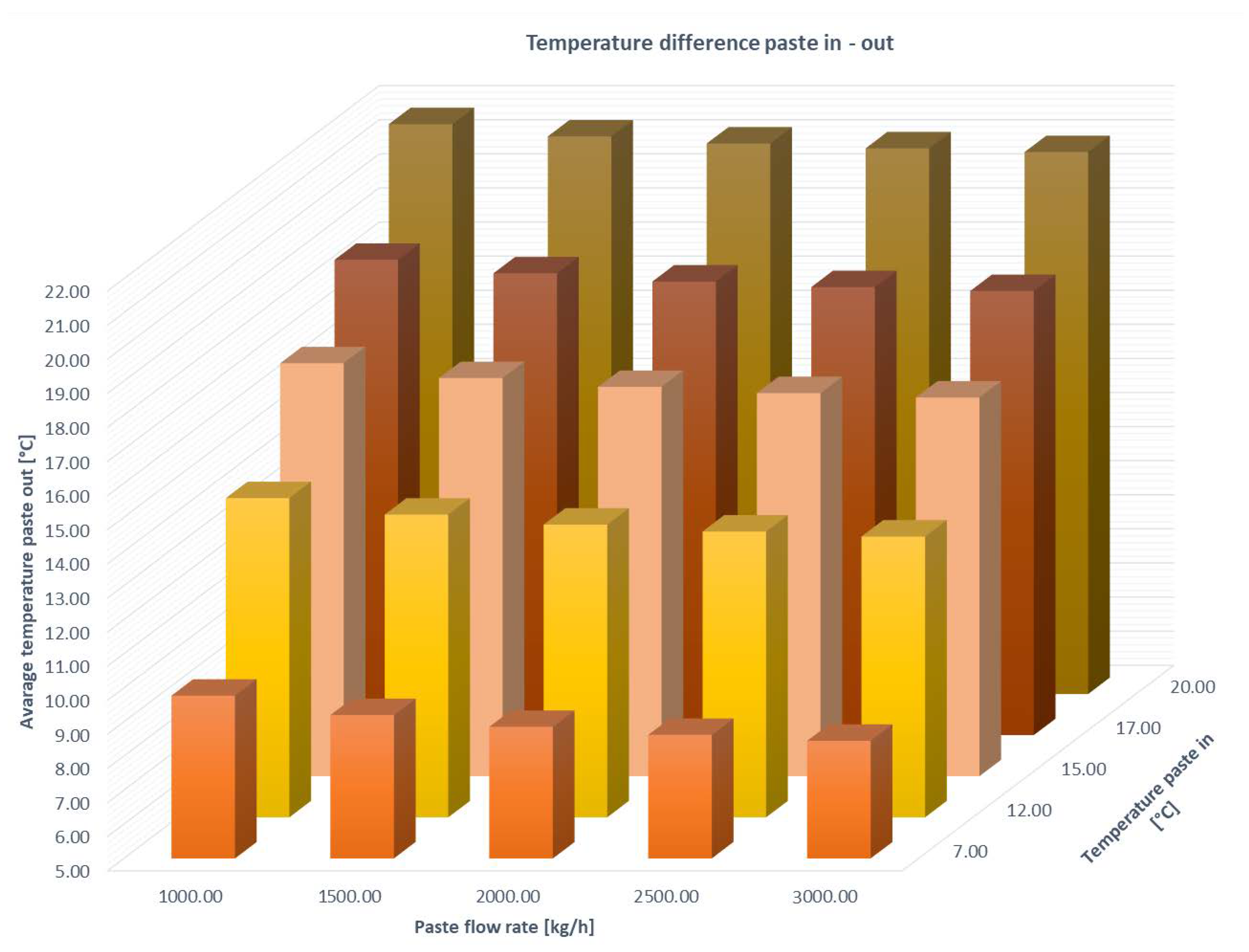
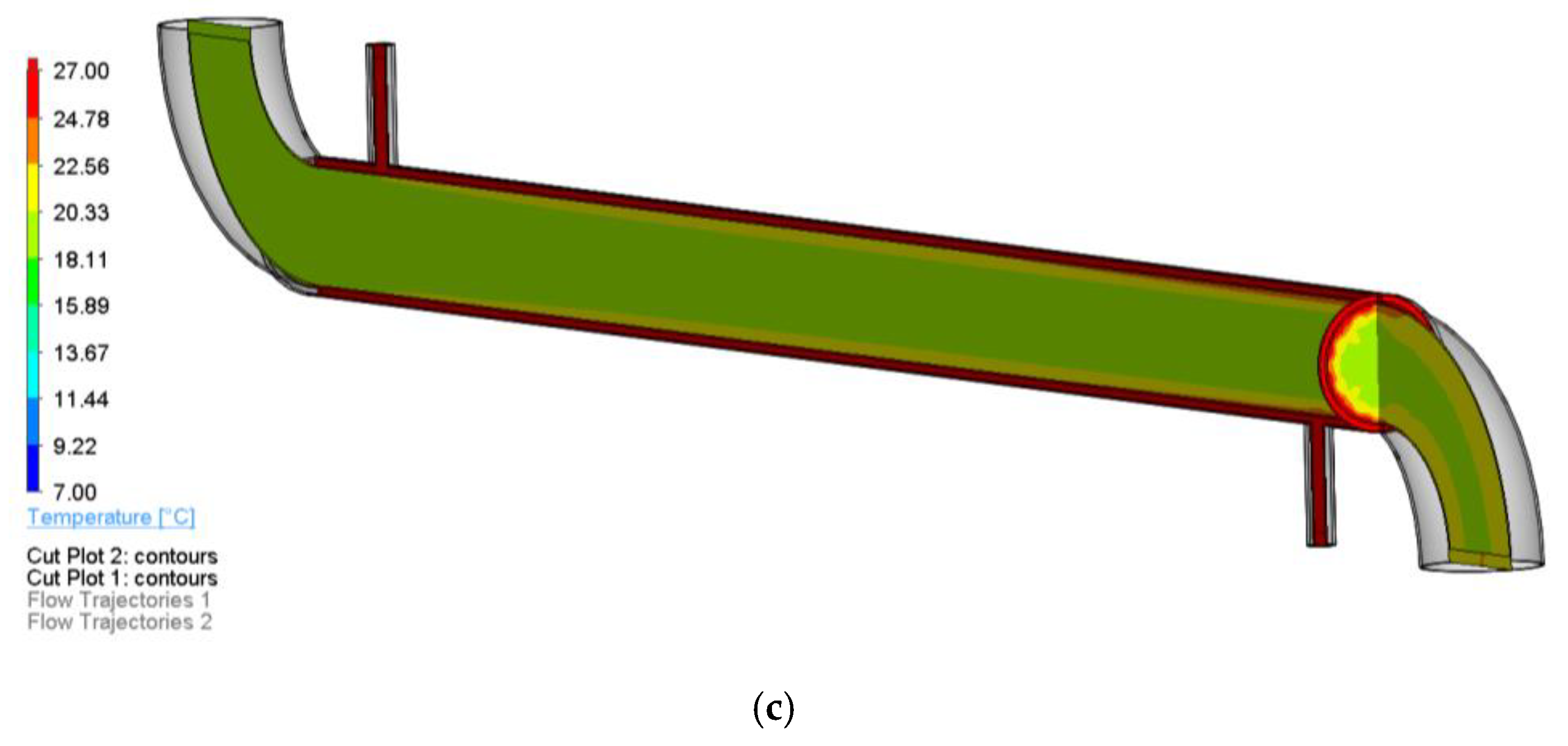
3.1. Temperature Variation in Different Scenarios

Figure 4 shows the average temperature of the olive paste at the outlet section of the inner tube under different inlet conditions. As expected, the difference in temperature between the inlet and the outlet (ΔT_p) decreases as the paste flow rate and its inlet temperature increases. Indeed the water, which flows with a mass flow rate of about 1.8 kg/s, has an inlet temperature that is kept to 40 °C in each scenario. However, it is possible to note that the inlet temperature of the paste has a lower influence on the ΔT_p, especially when the paste flow rate increases. At 3000 kg/h, the maximum ΔT_p is 1.45 °C when the paste enters at 7 °C, and ΔT_p is 0.90 °C when enters at 20 °C. This means a difference of 0.55 °C between the extreme case. Instead, when the minimum flow rate is used (i.e., 1000 kg/h), ΔT_p is 2.78 °C when the temperature of the paste at inlet is 7 °C and 1.71 at 20 °C. In this case, the difference between the extreme case is about 1.1 °C. This means that when the paste flow rate increases, to avoid an excessive increase in the heat exchange surface, it is necessary that the system improves the heat transfer. In fact, it is not desirable to increase the temperature of the service fluid in order to avoid compromising the product quality and prevent extensive fouling on the internal surface of the inner tube.

As stated, the above is confirmed by the results reported in Figure 5a–c, which shows the temperature contours inside the heat exchanger when the paste flow rate is 3000 kg/h, and the inlet temperature is 7, 15 and 20 °C, respectively. Two cut plots, the first along the longitudinal middle plane and second along the cross section at the end of the straight part of the heat exchanger, describe well the temperature distributions. It should be noted that the core temperature of the product remained virtually unchanged from entry to exit. This means that to obtain the desired temperature throughout the product, a part of it (near the internal surface) will inevitably undergo a qualitative degradation, compromising the quality of the olive oil extracted. In fact, it is easy to note that a large amount of the product (about 80%) still remained at the inlet temperature. The temperature increases from the middle towards the periphery of the section.

When the inlet temperature is 15 °C, the product near the wall experiences a maximum temperature of about 20.6 °C (Figure 5b), which becomes about 24.5 °C when it enters at 20 °C (Figure 5c). This is due to the rheology of the paste, which always produces a laminar flow and limits mixing, resulting in the absence of uniformity of heating for all portions of olive paste. The laminar flow of the olive paste is also demonstrated by Figure 6a,b, which shows the path lines and velocity values of both olive paste and water. Figure 6a shows very low variation of velocity in the straight part of the inner tube, with a slight variation in the elbows due to gravity. The average velocity of the paste in the inner tube is about 0.14 m/s, while the water flows (Figure 6b) at about 9 m/s in the supply tube, and ones in the jacket undergo a sudden reduction (reaching about 1.5 m/s in the middle of the straight part) and then rise again in the outlet tube.

Figure 7a shows the shear rate, which decrease moving through the center of the tube, since the velocity variation between the fluid layers at the center is lower than that near the wall. As a consequence, the dynamic viscosity distribution increases at the center due to the pseudoplastic behavior (viscosity increases when the shear rate decreases), as shown in Figure 7b.

The absence of heating uniformity of the olive paste leads to further considerations about the olive oil quality. Indeed, generally, the olive paste is heated at a temperature ranging from 24 to 27 °C or, in any case, on pre-set temperature values not to be exceeded by connecting in series more than one module. This range of temperature is strictly related to the olive oil quality that is consumed worldwide due to its appreciated sensory attributes and health benefits due to its fatty acid and richness in volatiles and phenolic compounds. To ensure the high content of phenolic and volatiles compounds, the extraction conditions and the temperature must be optimized. To this end, various studies have shown that malaxation at temperatures above 27 °C does not significantly increase the oil yield but leads to a gradual and significant reduction in the phenolic content as reported in [38,39,40,41,42]. In particular, in [40], it was found that temperatures ranging from 22 to 30 °C produced an increase in phenols of about 26%, while the C6 aldehydes decreased by about 18%.

In [43], the authors analyzed four different varieties of olives identifying the optimal values of temperature and oxygen concentration in the malaxer to maximize the main chemical parameters related to the oil quality, such as the phenolic and the volatile compounds. The authors found for each cultivar the following optimal temperature and oxygen levels: 33.5 °C and 54 kPa of oxygen (Peranzana), 32 °C and 21.3 kPa (Ogliarola), 25 °C and 21.3 kPa (Coratina) and 33 °C and 21.3 kPa (Itrana). These results demonstrate the importance of optimizing the homogeneity of temperature to enhance the quality parameters.

The non-uniform heating of high-viscosity fluids in a tube-in-tube heat exchanger suggests the importance of providing for the insertion of some mixing device able to stir the paste and ensure a better temperature distribution in the product. In addition, such a device could represent a good aid to prevent the fouling of inner surface of the heat exchanger. To this purpose, the use of a scraped surface heat exchanger (SSHE), which has a rotor coaxially inserted in the internal tube equipped with scraping blades, may be appropriate for olive paste pretreatments. In fact, SSHE models may provide a suitable solution to enhance the heat transfer in highly viscous or sticky fluids, where due to the low Reynolds number values, the fluid advances in a laminar regime, limiting the heat exchange as reported in [44,45,46]. An SSHE equipped with alternate blades particularly suited to treat high viscous fluids (hazelnut paste) has been developed in [23]. However, the hazelnut paste does not reach the viscosity values of the olive paste, especially at low shear rates. Furthermore, the typical SSHE blading should be carefully studied to avoid undesirable effects due to the presence of the pits.

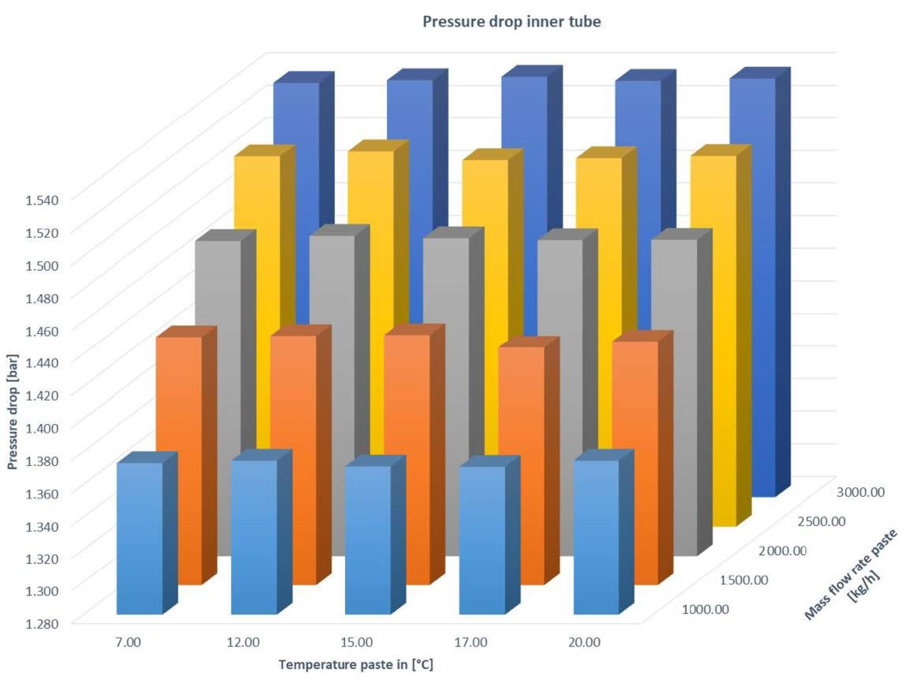
3.2. Pressure Variations in Different Scenarios

Figure 8 returns the total pressure at the inlet of the inner tube of the heat exchanger. By considering that the olive paste is discharged at atmospheric pressure (1.01 bar), the pressure drop of a single module ranges from 1.37 up to 1.53 bar. These values are obtained by considering the properties of the olive paste of Table 2, assumed as constants. In particular, the rheology of the paste was selected in order to simulate a very severe condition. This can happen especially in the subcontracting work, where private customers go to the local oil mill to process their olives. In real application, the number of modules could be two to six depending on the olive paste mass flow rate. Since the pressure drop increases linearly with the length of the inner tube (elbow pressure drops can be represented in pipe equivalent length), this produces a very high-pressure drop and could force the replacement of the cavity pump coupled to reinforced polypropylene pipes, which are widely used in oil mills, with a piston pump coupled to steel pipes to allow the use of the heat exchanger. This would entail an increase in costs for the oil mill. Therefore, introducing a device that improves the transport of the fluid in the heat exchanger to facilitate the work of the pump seems to be appropriate.

4. Conclusions

In the olive oil extraction process, the use of a tube-in-tube heat exchanger represents an opportunity to overcome the negative aspects arising during the malaxation phase and improve the process efficiency and the olive oil quality. For this purpose, in the last few years, the tube-in-tube heat exchanger has been increasingly used in the olive oil extraction industry for reasons related to its ease of use and low cost. However, some difficulties in its use have been encountered especially in batch processing due to the variation in the temperature of the inlet olive pastes and the feeding flow rate of the heat exchanger.

In this research, the CFD simulation allowed us to evaluate the temperature distribution and pressure drop of a tube-in-tube heat exchanger by varying the inlet temperature and mass flow rate of olive paste, which is notoriously a very viscous fluid.

The analysis of the outlet temperature of the olive paste shows the absence of uniformity of temperature reached by the different portions of pasta in relation to the position occupied in the exchanger. This consequently involves temperature increases on portions of pasta near the inner surface of the pipe wall, with negative consequences on the quality of the oil obtained.

Even considering the pressure head at the inlet of the inner tube, in all conditions, the authors point out that the use of a tube-in-tube heat exchanger, as it is, appears to be inappropriate.

Considering the results of CFD analyses, the authors suggest the desirability of using a scraped surface heat exchanger on olive pastes that comprises a rotor coaxially inserted in the internal tube to clean the inner surface of the stator avoiding particle deposition and, consequently, the occurrence of backmixing phenomena improving the heat transfer coefficient. The use of a device inside the exchanger should avoid deposition and cooking of olive paste particles, preserving the oil quality. In addition, it would facilitate the transport of the olive pastes, standardizing the supply pressures.

Definitely, CFD analysis has represented a valid tool to identify critical issues to be solved in order to facilitate the introduction of a new technology in the olive oil extraction industry.