Using UAV to Detect Solar Module Fault Conditions of a Solar Power Farm with IR and Visual Image Analysis

Abstract

In recent years, solar energy has been regarded as one of the most important sustainable energy sources. Under the rapid and large-scale construction of solar farms, the maintenance and inspection of the health conditions of solar modules in a large solar farm become an important issue. This article proposes a method for detecting solar cell faults with unmanned aerial vehicle (UAV) equipped with a thermal imager and a visible light camera, and providing a fast and reliable detection method. The detection process includes a new concept of real-time monitoring of the detected area and analysis of the health of solar panels. An image process is proposed that may quickly and accurately detect the abnormality of a solar module. The whole process includes grayscale conversion, filtering, 3-D temperature representation, probability density function, and cumulative density function analysis. Ten cases in real fields have been studied with this process, including large scale solar farms and small size solar modules installed on buildings. Results show that the cumulative density function is a convenient way to determine the health status of the solar panel and may provide maintenance personnel a basis for determining whether replacement of solar cells is necessary for improving the overall power generation efficiency and simplify the maintenance process. It is worth noting that image recognition can increase the clarity of IR images and the cumulative chart can judge the defect rate of the cell. These two methods were combined to provide an instant, fast and accurate defect judgment.

1. Introduction

In recent years, many countries are actively developing renewable energy-related industries, and the construction of solar power plants is regarded as an important part of it. Taipower (a government power agency in Taiwan), for example, has stated that 2019–2020 is a bumper year for large-scale development projects, and it is expected to achieve the target of 2.2 GW solar installations set by the Ministry of Economic Affairs. Meanwhile, Taipower is expecting to complete its annual production plan of 6.5 GW before the end of 2021 [1]. It is believed that solar energy will become one of the most important renewable energy sources in Taiwan. However, the maintenance and monitoring will be a challenge as many large scale solar farms are operated and built in remote area and some panels are even installed on top of high rise buildings. The panel temperature is an important factor to determine its efficiency. For example, when the temperature increases by 1 °C, the power generation efficiency of solar modules decreases by 0.5% [2,3,4]. Therefore, an accurate and efficient way of monitoring and identifying the failure of solar modules is essential [5]. In addition, rapid detection of solar module failures can extend the service life and maintain the performance of the solar system [6]. To improve the detection efficiency, this paper proposes a fast, time-saving and real-time detection system to identify the failure status of solar panels. In this study, a drone equipped with a set of high-definition cameras with infrared and visible light functions was adopted to inspect the health conditions of a solar farm. Advantages of using drones include large area coverage, high flexibility, light weight, and fast speed, and thus module defect detection can be performed in a relatively short time after the shooting status is sent back to the ground station [7]. Lastly, the image analysis with MATLAB is conducted to determine the status of these modules.

Using UAV to monitor a wide area of solar panels has been investigated by a lot of researchers previously. Libra et al. has developed a rapid inspection system with the help of drone to inspect the solar power plant at the Czech University of Life Sciences in Prague and the PV power plant in Ladná [8]. Their findings agreed with the situations that were found in real field inspection. Their work was conducted only inside the laboratory and on the roof of the building and no real data on real fields were collected and analyzed. The authors of that paper consider roofs to be a very convenient place to install small PV power plants that can be integrated into buildings. They perceived the usage of agricultural land for large PV power plants is far less appropriate. Alsafasfeh et al. also proposed a real time inspection and fault detection system for PV modules [2]. Their system contains a thermal and a CCD camera. Reports mentioned that defects have been identified accurately in the PV modules using the proposed real time system. The proposed drone mounted system is capable of analyzing thermal and CCD videos in order to detect different faults in PV systems, and give location information in terms of panel location by longitude and latitude. Niccolai et al. proposed a UAV-Based Digital Mapping system [9]. It allows easy access and completion of the information present in the database. This information management system and PV plant digitalization process are able to analyze and index the IR in the database and obtained visual images in photovoltaic plant monitoring properly.

Monitoring the status of solar modules has become an important issue recently and many kinds of research have been conducted to find a quick and reliable way for faults detection. A review of the recently published papers is given in

Table 1. Comparison of related references on solar panel monitoring.

References	Method
	UAV	IR Image Defect Detection	Other Defect Detection
Alsafasfeh, M., et al. [2]	yes	yes
Hwang, M.-H., et al. [4]		yes	bypass diode
Libra, M., et al. [8]	yes	yes
Niccolai, A., et al. [9]	yes		digital map
Vieira, R.G., et al. [10]		yes	bypass diode
Navid, Q., et al. [11]		yes
Henry, C., et al. [12]	yes	yes
Pierdicca, R., et al. [13]	yes	yes	deep learning
Jeong, H., et al. [14]	yes	yes	diagnosis
Boulhidja, S., et al. [15]		yes
Tsanakas, J.A., et al. [16]	yes	yes
Tsanakas, J.A., et al. [17]		yes
Gallardo-Saavedra, S., et al. [18]		yes
Ballestín-Fuertes, J., et al. [19]			EL 1
Herraiz, Á.H., et al. [20]	yes	yes
Fernández, A., et al. [21]	yes	yes

¹ Electroluminescence Technique.

which compares the way these investigations were carried out. It seems quite clear that UAV is a very convenient tool for large scale monitoring that many researchers use UAV for collecting data. In addition, IR image detection is popular that most researchers use it for fault detection.

2. System Configuration and Methods of Analysis

The innovative method of this research is to combine UAV (

Table 2. Unmanned aerial vehicle (UAV) specification and parameters.

Parameter	Value
Type	Six-axis drone LION-690
Propeller	13 inch × 6
Weight	6 kg
Load	2 kg
Mission Altitude	1–10 m
Cruise Speed	5–10 m/s
Sensor Resolution	160 × 120

), a dual lens camera (FLIR Duo R) which is equipped with visible light and IR lens, with real-time analysis software for solar module detection. Figure 1 shows the UAV and camera containing infrared and visible light adopted in this study. The schematic diagram of the proposed solar modules monitoring/UAV system is shown in Figure 2. This real-time analysis system requires a ground station for control and analysis. The ground station includes a control receiver and a computer equipped with MATLAB software. When the drone flies over solar power modules and takes photos with dual lens above, images are instantly transmitted to the ground station through the integrated radio frequency (RF) channel for analysis. The ground station can record modules’ images and exam the health conditions of the modules in real time. Recorded images are analyzed in a computer equipped with MATLAB software. The output results may provide maintenance personnel a good reference for determining whether replacement of the module is necessary for improving the performance and extending the life of the solar module. In addition, fixing early-detected defects in time may prevent the deterioration of the module and reduce maintenance costs [8,22]. However, it is difficult to interpret the acquired IR image due to uncertain factors such as image quality, weather conditions, shadows during inspection and reflection of sunlight. Therefore, it would be beneficial using software tools to facilitate the defect and fault detection process [23]. On the other hand, IR images can help to detect hot spots in the solar module while the visual light images can differentiate the spots caused by light reflection and abnormal high temperature. These hot spots provide indications of abnormal operations that may result in a reduction of power generation or damage to the solar system. The main steps for the proposed system are shown in Figure 3.

The main purpose of implementing image analysis technology is to detect defects in solar modules. This process is divided into two stages. The first stage is to find out the status and the location of defects in a solar module with Gaussian filter image analysis. This method has been confirmed in a previously published paper to identify defects [8]. The second stage is an innovative method for evaluating the extent of these verified defects.

2.1. Gaussian Filter Image Analysis Method

The authors of this paper have proposed a real-time image analysis system for solar panel fault detection with UAV previously [23]. Three different filtering methodologies were compared in that study, and the Gaussian filter was found to be the most suitable for detecting the high temperature spots on solar panels. In this study, Gaussian filter was adopted for the pre-treatment of the IR image, and the temperature distribution of the panel was presented with a histogram and a cumulative curve.

The pixel in an IR image is composed of different ratios of RGB. In response to this, converting the image from RGB to grayscale becomes the first step. This procedure not only enhances the resolution of the image but also facilitates color judgment of the image. Synchronously, filters are necessarily applied to eliminate noise and reduce the sharpness of the image. In fact, filtering techniques are adopted to pre-process the image prior to the detection of faults. In this study, Gaussian filters are applied to reduce noise and other unnecessary details in IR images. Normally, defects such as hot spots and cracks can affect the temperature uniformity on the solar panel module and result in different colors in the IR image. However, noise may also occur in the IR image that real defects may be misinterpreted. Normal components and defective areas on the solar panel module, without the interference of noise, can be clearly distinguished under the filtered image, as shown in Figure 4. The original IR image was grayscale-processed follow by a division of black and white pixels of the image, as shown in Figure 4b, representing cold areas and hot spots on the surface of the solar module respectively [8]. To show the defect more clearly, it is necessary to convert it to an RGB image as shown in Figure 4c. After the conversion, the green area shows up to represent cold zone and the red area the hot zone. The correspondence between color and temperature is shown in the color bar. The lowest temperature in this image is 35 °C and the hottest area is at 55 °C.

Figure 4a is the original IR image which was grayscale-processed. Basically the panel is of uniform temperature with color of yellowish orange but some areas with bright color are also displayed, indicating that higher temperature regions are distributed in the panel. Figure 5b shows an image converted to grayscale after Gaussian filtering.

2.2. Innovative Methods and Experimental Setup

In this research, an algorithm is proposed to process IR images of solar modules in Matlab environment. The following two conditions must be confirmed before applying this method. First, ensure that irradiance is I ≥ 700 W/m² before carrying out the investigation [23,24]. Second, it is necessary to measure the intensity of solar radiation and set a temperature meter on the solar module before performing an inspection. This is because the environmental temperature will affect the temperature on the solar module, and thus causing deviations of infrared display temperature. Therefore, drone inspection must be conducted under the conditions mentioned above. Its purpose is to ensure that the temperature reading is correct when performing MATLAB image analysis.

3. Results of Field Tests

In this study, thermal imaging analysis of solar photovoltaic modules was performed by infrared cameras (FLIR Duo R) mounted on the UAV, and IR images were immediately transmitted back to the ground station for analysis. After receiving the IR image, the ground station performs grayscale processing and Gaussian filtering. At the same time, 3-D images or color images are presented to increase the identification of defects. Finally, the IR image is analyzed through the image processing techniques introduced above. The location of the defect area is identified and the ratio of the fault area to the total area of the solar module is obtained.

Experiments were conducted in two stages. In the first stage, modules with known conditions were applied to locate the characteristics of IR images. Four modules were used in this stage, including one in good condition, and three with defects that are already known. In the second stage, unknown modules were applied for testing the validation of the process to improve the reliability and validity of this study. A total of six modules were applied in this stage.

3.1. The First Stage Experiments

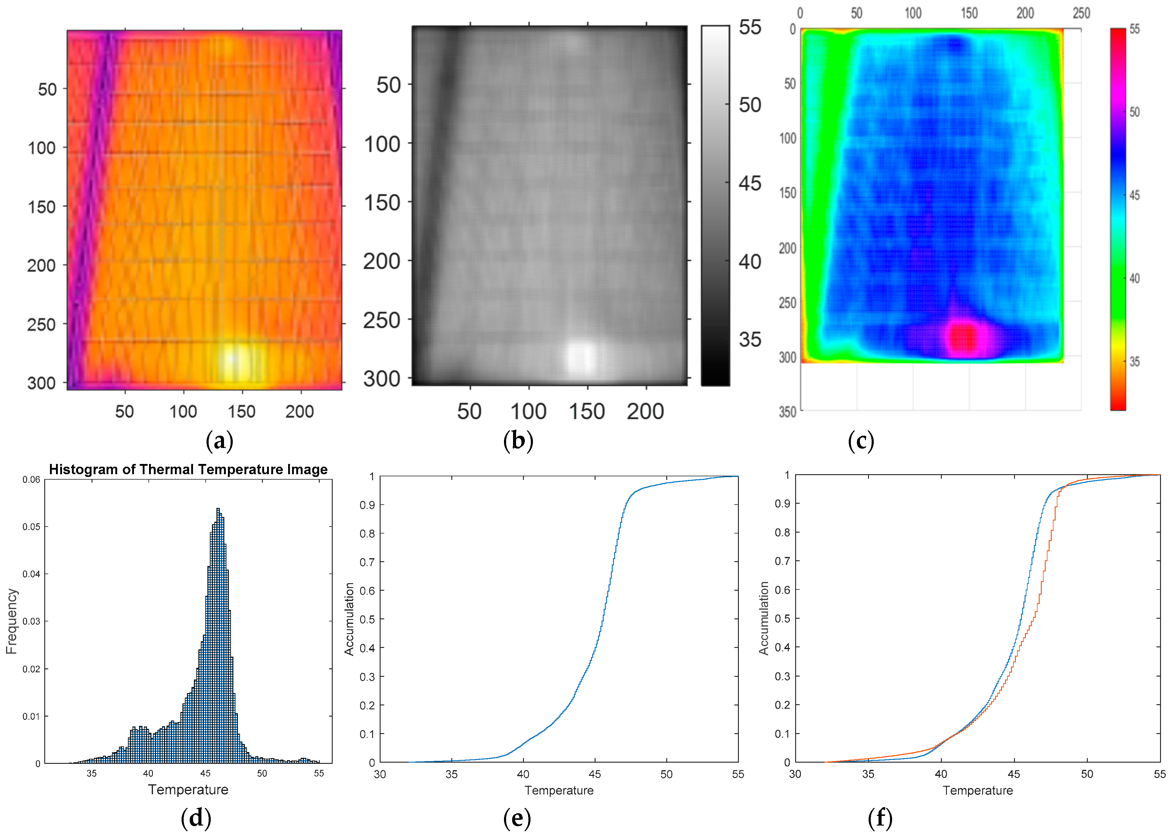
Figure 5 shows the image of a healthy solar module. Figure 5a is the original IR image of this healthy module in normal operation. It shows that basically the panel is of uniform temperature with color of yellowish orange. However, some areas with bright color can also be observed, indicating that higher temperature regions are distributed in the panel. Figure 5b is an image converted to grayscale after Gaussian filtering. The temperature distribution in Figure 5b was calibrated with a thermometer shown in Figure 2. It shows that the whole panel was at around 48 °C while the normal operating temperature of a healthy solar module is 45 °C to 49 °C. However, there is a cell-sized hot spot in the top middle area of this panel and the accurate measurement of the area of this hot spot is 1.67% of the total area with a temperature 55 °C. The reason is that at the back of the panel, there is a junction box located just opposite to the hot spot region and the temperature in this region is comparatively higher than its neighborhood due to the thermal insulation of the junction box, and therefore it is not a malfunction or abnormality.

Solar cells are basic units of a solar panel. Several units of cells are connected in series and parallel, and encapsulated together to form a solar photovoltaic panel module. In this study, the experimental solar module is composed of 6 × 10 cells, making one solar module contains 60 cells. Failure of a single cell would account for 1/60 of the fault area (about 1.67%). The aforementioned hot spot occupied 1.67% of the total area, indicating only one cell is at relatively high temperature. As a result, the innovative method of this research can find not only hot spots, but also determine whether it is a hot spot caused by cell failure or contamination.

Figure 5c shows a 3-D image of the solar module in normal operation after Gaussian filtering. The temperature variations on the panel surface is converted to a three dimensional hills and valleys to signify the high temperature regions that could not be noticed in the two dimensional figure as shown in Figure 5b. The peak on the upper middle is the hot region caused by the junction box on the opposite side of panel as mentioned before. Figure 5d shows the histogram of the probability density of the calculated temperature value in each pixel. The temperature of a solar module in normal operation is not a normal distribution, but rather it looks like a Beta distribution with α = 8 and β = 2. The mean temperature is 48 °C with a deviation of −7 °C. The maximum temperature is 55 °C and the minimum temperature is 35 °C. The probability density function (PDF) of temperature distribution is a characteristic of a solar panel. In this paper, the PDF and the associated cumulative function are used as an important index to determine the health condition of a solar panel. Figure 5e displays the cumulative distribution function (CDF) of the temperature distribution. It is found that 98.5% of the pixels are under 50 °C and only 1.5% of pixels exceed 50 °C. The above description shows that 98.5% of the panel is within the normal area, as displayed in Figure 5d–e. It is noted that the hot spot area caused by the junction box on the back of the solar module is about 1.5%. Since the junction box is not a malfunction of the panel, we may therefore conclude that 1.5% of hot spot might not be a malfunction problem in the CDF curve. Further examination is needed to check if it is a normal operating panel.

The second experiment was conducted on three panels that have known defects. The location of these panels is on the GPS coordinates of 24°12′31″ N and 120°29′40″ E with an altitude of 5 m. The experiment was carried out on April 1, 2020, at 11 am. The outdoor temperature is 28 °C. The surface temperature of the normal operating solar module is 45~ 49 °C, and the surface temperature of the abnormal solar module is 50~55 °C with irradiance of 815 W/m².

The first panel has a defective cell in the lower middle of the panel. Figure 6a shows the original IR image with a clear and bright area shown in the lower middle that corresponds to the defected cell while a less bright area located in the upper middle is the junction box as mentioned before. Purple lines on the left and right margins are frames of the panel. Figure 6b shows an image converted to grayscale after Gaussian filtering. Grid lines of the panel are blurred due to the filtering effect but the bright region still appears clearly. Figure 6c displays a color image after Gaussian filtering to differentiate temperatures and the image tells that the hot spot is at about 55 °C and panel frames are at the temperature of 40 °C while the rest of the panel is at around 45~50 °C.

Figure 6d is the histogram of the temperature distribution. The PDF curve still looks like a beta distribution function but a bump can be found at 40 °C which was not shown in Figure 5d of a normal operating panel because panel frames were not included in Figure 5. The mean temperature of the whole panel is 46 °C with the deviation of −9 °C. The maximum temperature is 55 °C and the minimum temperature is 32 °C. Figure 6e is the cumulative temperature distribution that the mean temperature, maximum temperature and minimum temperate are very close for a normal operating panel and a panel with a known defected cell. However, hot spots are clearly shown on the solar module in Figure 6a–c. Through the cumulative chart, it is found that the percentage of hot spot area is over 3.1%, indicating there are two cells with high temperature. We already knew that one of the cells is caused by the junction box and there should be another cell in abnormally high temperature. To highlight the difference between a normal panel and a panel with known defected cell, we have compared the CDF curves of these two panels in Figure 6f. Result shows that the percentage of the area over 50 °C is a good index to determine cell abnormality or failure. The above description shows that 96.9% of the panel is within the normal area, as displayed in Figure 6d–e.

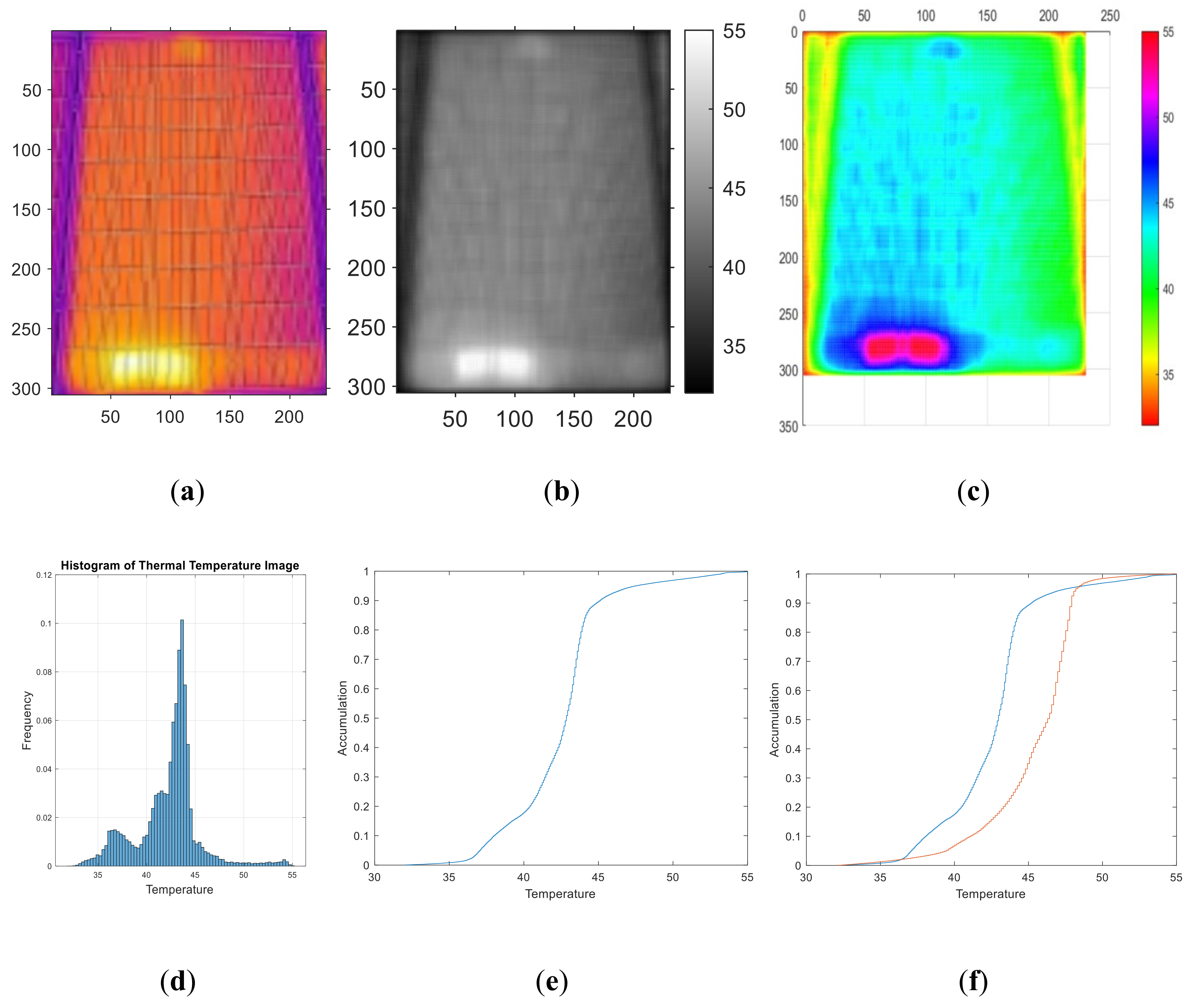
The second panel has two defected cells located in the lower middle of the panel. Figure 7a shows the original IR image with a clear and bright area shown in the lower middle that corresponds to the defected cell. Figure 7b shows an image converted to grayscale after Gaussian filtering. Figure 7c shows a color image after Gaussian filtering that the hot spot is at about 55 °C. Panel frames are at the temperature of 38 °C and the rest of the panel is at around 45~50 °C. Figure 7d displays the histogram after calculating the temperature value of each pixel. The PDF curve still looks like a beta distribution function and the bump with 38 °C is panel frames. The mean temperature is 43 °C with the deviation of −12 °C. The maximum temperature is 55 °C and the minimum temperature is 32 °C. Figure 7e displays the cumulative temperature distribution that the percentage of hot spot area over 50 °C is 3.4%, indicating there are more than two cells with high temperature. Lastly, Figure 5e and Figure 7e are superimposed to form Figure 7f for comparing normal and abnormal conditions. Figure 7e shows that the area over 50 °C is about 3.4%, which is higher than the 1.5% threshold presumed for a normal solar module, indicating that more than one cell has abnormality or failure. The above description shows that 96.6% of the panel is within the normal area, as displayed in Figure 7d–e. This is consistent with Figure 7a–c, showing that the bright area of the hot spot is clearly visible.

The third panel has no defected cells but several drops of bird guano can be observed on the central middle of panel. This experiment tested irregular shaped hot spots that are often found in remote area. Figure 8a shows the image of the panel obtained through a visual light camera. It is found that bird droppings could not be easily differentiated from its background by visual inspection because both the bird droppings and cells are of black color. Figure 8b shows the original IR image with a bright color region at the central middle part of the panel which is the location of bird droppings. However, it is not brighter than its surrounding and it could be easily overlooked only by visual inspection of the IR image. Figure 8c shows an image converted to grayscale after Gaussian filtering and it shows a clearer image of bird droppings than that in the original IR image because the grayscale magnified the color difference of image. Figure 8d displays an artificial color image based on the grayscale of each pixel after Gaussian filtering. In Figure 8c,d, the hot spot area is more obvious than that in Figure 8b (as shown in the red circle). Unlike the rectangular shape of hot spot shown in Figure 6c, which is caused by failed cells, the hot spot in Figure 8e is of irregular shape. Figure 8f displays the histogram of the PDF of the temperature values in each pixel and the bump with 45 °C is panel frames. The mean temperature is 48 °C with the deviation of −7 °C. The maximum temperature is 55 °C and the minimum temperature is 31 °C. The cumulative chart of CDF is shown in Figure 8f. The percentage of the hot spot area over 50 °C can be obtained from the cumulative curve, which is 5.5% in this panel. The above description shows that 94.5% of the panel is within the normal area, as shown in Figure 8e,f. Lastly, Figure 5e and Figure 8f are superimposed to form Figure 8g for comparing normal operation and abnormal conditions. It seems that there are about 3–4 abnormal cells and the hot spot area in Figure 8d is irregular and thus it is concluded that those 3–4 abnormal cells are caused by stains.

The innovative finding of this research depicts the following observations. When one cell (about 1.67%) on the solar module exceeds 50 °C, it means that a hot spot or abnormality occurs in one cell of the module, which may reduce the power generation of the module. The innovative method of this research can find not only hot spots, but also estimate the proportion of hot spots on a solar module. This may avoid the misinterpretation of hot spots caused by some small stains (such as bird droppings, branches, leaves, or dust) as cell failure. If the hot spot proportion is not multiples of 1.67% and the shape of hot spot is irregular, it can be determined that the solar module is contaminated and would only require simple cleaning. In fact, during the operation of the solar module, as long as the hot spots caused by cell failure or stains are distinguished, the correct judgment can be made for cleaning or maintenance. As a result, the service life of solar modules is increased and costs are reduced. Some of the results are presented in the following cases.

3.2. The Second Stage Experiments

In the second stage of experiments, modules with unknown conditions were used to test the findings of the first stage. A total of six modules were tested in this stage. Experiments were conducted at different locations in the verification field. In each case, one to three images were selected for verification. Verification locations and results are illustrated in the following cases:

In the first case, the power generation efficiency is low but no obvious damage was found by visual inspection. The location of these panels is on the GPS coordinates of 24°12′31″ N and 120°29′39″ E with an altitude of 5 m. The nominal output of this solar farm is 6486 kWp. The experiment was carried out on 1 April 2020, at 12 a.m. The outdoor temperature is 29 °C. The surface temperature of the normal operating solar module is 45~49 °C, and the surface temperature of the abnormal solar module is 50~56 °C with irradiance of 827 W/m². Three panels were inspected in this paper following the procedure mentioned above.

The first panel has three hot spots with the brightest spot at the bottom left, followed by the bottom right and the top middle. Figure 9a shows the original IR image with a clear and bright area in the bottom left that corresponds to the defected cell while a less bright area located in the upper middle is the junction box as mentioned before. In addition, a defected cell in the lower right of the panel can also be observed in the IR image with purple lines on the left and right margins as frames of the panel. Figure 9b shows an image converted to grayscale after Gaussian filtering. Grid lines of the panel are blurred due to the filtering effect but the bright region still appears clearly. Figure 9c shows a color image after Gaussian filtering to differentiate the temperature variations that the hot spot is at about 56 °C. Panel frames are at the temperature of 40 °C and the rest of the panel is at around 40~49 °C. Figure 9d displays a histogram of the temperature distribution. The PDF curve still looks like a beta distribution function. However, a bump can be found at 38 °C which was not shown in Figure 5d of a normal operating panel because panel frames were not included in Figure 5. The mean temperature is 45 °C with the standard deviation of −11 °C. The maximum temperature is 56 °C and the minimum temperature is 30 °C. Figure 9e displays the cumulative temperature distribution that the percentage of hot spot area over 50 °C is 3.3%, indicating there are more than two cells with high temperature. Finally, Figure 5e and Figure 9e are superimposed in Figure 9f for comparing normal and abnormal conditions. Figure 9e shows that the area over 50 °C is about 3.3%, which is higher than the 1.5% threshold presumed for a normal solar module, indicating that more than one cell has abnormality or failure. The above description shows that 96.7% of the panel is within the normal area, as shown in Figure 9d,e. This is consistent with Figure 9a–c, showing that bright area of hot spot is clearly visible.

The original IR image of the second panel at the same location is shown in Figure 10a with a clear and bright area in the bottom right that corresponds to defected cells while a less bright area located in the upper middle is the junction box as mentioned before. Figure 10b shows an image converted to grayscale after Gaussian filtering that the bright area still appears clearly after filtering. Figure 10c shows a 3-D color image of the temperature distribution with a high rise hill occurs at the hot spot at about 55 °C. Panel frames are at the temperature of 40 °C while the rest of the panel is at around 43~48 °C. Figure 10d shows a histogram of the temperature distribution. The PDF curve still looks like a beta distribution function and the bump with 40 °C corresponds to panel frames. The mean temperature is 44 °C with the deviation of −11 °C. The maximum temperature is 55 °C and the minimum temperature is 30 °C. Figure 10e displays the cumulative temperature distribution that the percentage of hot spot area over 50 °C is 2.8%, indicating there are two cells exceeding the temperature threshold. Finally, Figure 5e and Figure 10e are superimposed in Figure 10f for comparing normal and abnormal conditions. Figure 10e shows that the area over 50 °C is about 2.8%, which is higher than the 1.5% threshold presumed for a normal solar module, indicating that almost one cell has abnormality or failure. The above description shows that 97.2% of the panel is within the normal area, as shown in Figure 10d,e. This is consistent with Figure 10a–c, showing that bright area of hot spot is clearly visible.

The original IR image of the third panel at the same location is shown in Figure 11a with a clear and bright area in the bottom left that corresponds to defected cells while a less bright area located in the upper middle is the junction box as mentioned before. Figure 11b shows an image converted to grayscale after Gaussian filtering. The grid in this image is still clearly visible after Gaussian filtering because the resolution of the original picture is higher for the third panel and the bright region still appears clearly after filtering. Figure 11c shows a color image after Gaussian filtering to tell the temperature difference on the panel. It reveals that the hot spot is at about 54 °C. Panel frames are at the temperature of 40 °C while the rest of the panel is at around 45 ~ 49 °C. Figure 11d shows a histogram of the temperature distribution. The PDF curve still looks like a beta distribution function and the bump with 40 °C is contributed by frames of the panel. The mean temperature is 44 °C with the deviation of −10 °C. The maximum temperature is 54 °C and the minimum temperature is 30 °C. In addition, there is a clear bump at 54 °C, which is a defect caused by hot spots. At the same time, Figure 11e displays the cumulative temperature distribution that the percentage of hot spot area over 50 °C is 3.2%, indicating there are two cells exceeding the temperature threshold. Finally, Figure 5e and Figure 11e are superimposed in Figure 11f for comparing normal and abnormal conditions. In Figure 11e, the area over 50 °C is about 3.2% of the third panel, which is higher than the 1.5% threshold presumed for a normal solar module, indicating that one cell has abnormality or failure. The above description shows that 96.8% of the panel is within the normal area, as shown in Figure 11d,e. This is consistent with Figure 11a–c, showing that bright area of hot spot is clearly visible.

A brief conclusion can be drawn in the first case: The procedure of IR image analysis can search panels that have cells exceeding the temperature threshold effectively, as well as panels that have been confirmed to be abnormal.

In the second case, the power generation efficiency is low and no obvious damage is found by visual inspection. The location of these panels is on the GPS coordinates of 24°05′45″ N and 120°23′11″ E with an altitude of 5 m. The nominal output of this solar farm is 40 MWp. It is the largest solar farm installed in Taiwan so far. The experiment was carried out on 7 April 7 2020, at 1 p.m. The outdoor temperature is 24 °C. The surface temperature of the normal operating solar module is 45~49 °C, and the surface temperature of the abnormal solar module is 50~55 °C with irradiance of 746 W/m². Only one panel was inspected with an IR image in this case.

Figure 12a shows the original IR image. The image of this panel looks different because the panel is installed horizontally instead of vertically at this location. There are lots of bright areas on this panel, but the number of hot spots cannot be immediately recognized in the image. Figure 12b shows an image converted to grayscale after Gaussian filtering. Grid lines of the panel are blurred due to the filtering effect but bright areas are more visible than infrared images. Figure 12c shows a color image after Gaussian filtering to demonstrate the temperature difference on the panel that the hot area is at about 55 °C. Panel frames are at the temperature of 43 °C while the rest of the panel is at around 45~49 °C. Figure 12d shows a histogram of the temperature distribution. The PDF curve still looks like a beta distribution function. The mean temperature is 50 °C. The maximum temperature is 55 °C and the minimum temperature is 40 °C. The average temperature of this panel is relatively high and there are many defective cells causing hot spots. Figure 12e displays the cumulative temperature distribution that the percentage of hot spot area over 50 °C is 53.8%, indicating more than half of the cells in this panel are defective. Finally, Figure 5e and Figure 12e are superimposed to form Figure 12f for comparing normal and abnormal conditions. Figure 12e shows that the area over 50 °C is about 53.8%, which is higher than the 1.5% threshold presumed for a normal solar module, indicating that 31 cells have abnormality or failure. The above description shows that only 46.2% of the panel is normal, as shown in Figure 12d,e. This is consistent with Figure 12a–c.

In the third case, the power generation efficiency is normal and no obvious damage is found by visual inspection. The location of these panels is on the GPS coordinates of 24°03′59″ N and 120°42′56″ E with an altitude of 169 m. The nominal output of this solar farm is 6 kWp. The experiment was carried out on 20 August 2020, at 10 a.m. The outdoor temperature is 28 °C. The surface temperature of the normal operating solar module is 45~49 °C, and the surface temperature of the abnormal solar module is 50~53 °C with irradiance of 776 W/m². Two panels were inspected with IR images in this case.

Figure 13a shows the original IR image of the first panel with a clear and bright area in the top middle that corresponds to a defected cell while the upper middle is the junction box as mentioned before. The dark purple lines around the cells are frames of the panel. Figure 13b shows an image converted to grayscale after Gaussian filtering but the bright region still appears clearly. Figure 13c shows a 3-D color image after Gaussian filtering to tell the temperature difference that the hot spot in the top middle is at about 53 °C. Panel frames are at the temperature of 43 °C while the rest of the panel is at around 45~49 °C. Figure 13d shows a histogram of the temperature distribution. The PDF curve still looks like a beta distribution function. The mean temperature is 42 °C with the deviation of −11 °C. The maximum temperature is 53 °C and the minimum temperature is 30 °C. Figure 13e displays the cumulative temperature distribution that the percentage of hot spot area over 50 °C is 1.6%, indicating there is only one cell exceeding the temperature threshold. Finally, Figure 5e and Figure 13e are superimposed in Figure 13f for comparing normal and abnormal conditions. It is found that the area over 50 °C is about 1.6%, which is close to the 1.5% threshold presumed for a normal solar module, indicating that there is no abnormality or failure. The above description shows that 98.5% of the panel is within the normal area, as shown in Figure 13d,e. This is consistent with Figure 13a–c, which shows that bright area of hot spot is clearly visible.

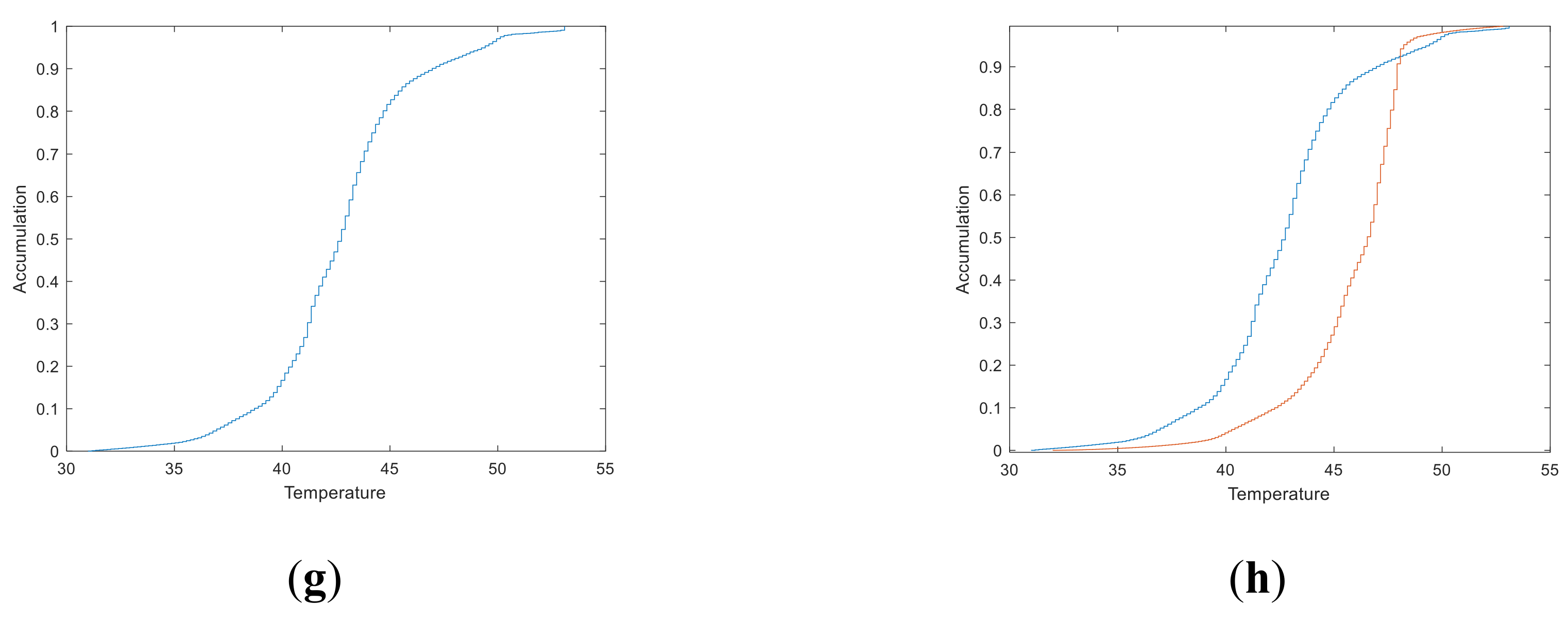
The second panel at the same location has a wide bright area in the upper part as shown in Figure 14a,b and it is a visible light image, not an IR image. This bright area is caused by the direct reflection of sunlight. Figure 14d shows the IR image of the same panel taken at the same time as the visual light image. The wide bright area of reflection disappears but a clear and bright zone with a smaller area still exists in the right middle that corresponds to defected cells. Figure 14e shows an image converted to grayscale after Gaussian filtering and the bright zone still appears clearly. Figure 14f shows a histogram of the temperature distribution. The PDF curve still looks like a beta distribution function and the huge bump with 41 °C is caused by panel frames. The mean temperature is 43 °C with the deviation of −10 °C. The maximum temperature is 53 °C and the minimum temperature is 30 °C. Figure 14g displays the cumulative temperature distribution that the percentage of hot spot area over 50 °C is 3%, indicating there is one cell with high temperature. Finally, Figure 5e and Figure 14g are superimposed in Figure 14h for comparing normal and abnormal conditions. Figure 14g shows that the area over 50 °C is about 3%, which is 1.5% higher than threshold presumed for a normal solar module, indicating that there is one cell abnormality or failure. The above description shows that 97% of the panel is within the normal area, as shown in Figure 14f,g.

However, this is a normal operating panel and there are no defected cells occurred. The results of IR image analysis seem to be contracted with the real situation, indicating that there is a blind spot for this analysis procedure that could happen when there is direct reflection of sunlight on the panel. To avoid this blind spot, it is suggested that the visible light image should be inspected to check whether there is any reflection on the panel before the IR image analysis is conducted. Therefore, the visible light images at different time periods can be used to determine whether it is reflective. For example, Figure 14c is the photo of the same modules, but the shooting timing is a few seconds later. We can see that the flare in Figure 14a disappeared in Figure 14c. If the flare is caused by any malfunctions, it would not disappear just a few seconds later. So we may determine that the flare is caused by direct reflection which is strongly affected by the angle of shooting. To ensure the completeness and validity of this analysis procedure, the image is removed to prevent misjudgment if the image of the panel has reflection when the photo is taken.

3.3. Case Integration

All data of experiments conducted in this paper were assembled for comparison as shown in

Table 3. Case integration table.

Stage	Experiments Group	Threshold Temperature (°C)	Accumulation Up to 50 °C (%)	Failure (%)	Number of Cell Failures
First stage	1	50.1	98.5	0	0
	2.1	50.0	96.9	1.6	1
	2.2	50.0	96.5	2.0	1–2
	2.3	50.0	94.5	4.0 1	-
Second stage	1.1	50.0	96.7	1.8	1
	1.2	50.0	97.2	1.3	1
	1.3	50.0	96.8	1.7	1
	2	50.0	46.2	52.2	31
	3.1	50.0	98.4	0	0
	3.2	50.0	97.0	1.5 2	-

¹ The case is determined as a contamination in the IR image. ² Misjudgment of defects caused by reflection.

. The Failure (%) is the ratio of the area that exceeds the temperature threshold. However, 1.5% of the hot spot area should be accounted for the junction box. Therefore, the Failure (%) is the hot spot area ratio after adjustment. In experiment 2.3, there were 4% defects and the actual defect is not a cell defect but rather is hot spots caused by bird dropping. This explains why this table excludes the number of cell defects. In addition, there is an occurrence of 3% defects in experiment 3.2 but it is not a cell defect but rather is a hot spot caused by reflected light. This explains why this table excludes the number of cell defects.

4. Discussions

The novelty of this paper is to propose an image process that can possibly detect the abnormality of a solar module quickly and accurately. The whole process includes grayscale conversion, filtering, 3-D temperature representation, probability density function, and cumulative density function. Different kinds of faults may be detected in this process. Unlike the preceding report [2], this article presents real-size outdoor PV array monitoring by drone. The health condition and defect ratio of each panel can be monitored, which is different from the previous report [8,9]. The advantage of the innovative method proposed in this paper is to apply an infrared imaging system with drone functions to detect faults in the solar power system and MATLAB image analysis software is adopted to analyze the IR image. Results show that in addition to the instantaneous acquisition of IR images, the health and defect area of the cell can also be determined clearly and defective solar panels can be compared through the cumulative chart data promptly. Furthermore, the procedure of IR image analysis can search panels that have cells exceeding the temperature threshold effectively, as well as panels that have been confirmed to be abnormal.

The cumulative chart is a convenient way to represent the temperature distribution on the module. The grayscale of the thermal image may show the abnormal area on the module. However, the representation is qualitative rather than quantitative. It is difficult to determine how severe the damage is based on qualitative representation. The cumulative curve proposed in this paper is a quantitative way to represent the temperature distribution on the module. One characteristic of the cumulative curve, which was not shown in the paper, is that we can mark any point on the accumulation curve to show the percentage of the area below the specified temperature. The maintenance staff may make decisions quickly and accurately based on the cumulative curve of each image. Ten cases have been tested in this paper and the results have confirmed the validity of this method. More cases of testing will be carried out in the future.

The detection of faults in solar modules by AI is a future trend. However, the original image contains too much information that it takes time to inspect the image by machine vision or other AI technology. The cumulative distribution function proposed in this paper is a new tool for the preliminary examination of thermal images. It is a much easier way to detect the abnormality of a solar module than the direct inspection with machine vision. Once it is determined by the cumulative distribution function that there is something wrong with the module, the machine vision can then be applied to inspect the thermal image to find out the location as well as the severity of faults.

5. Conclusions

A four-step procedure of image analysis is proposed in this paper. The original IR image is filtered and converted to grayscale image in the first step. The image is then converted to 3-D color to magnify the temperature difference in the second step. A histogram of thermal temperature distribution is then built in the third step to find out the percentage of high temperature area. A cumulative chart of the temperature distribution is finally built in the last step to determine the number of cells that may be abnormal or defective. A total of ten cases have been examined by this procedure. According to results of analysis, not only the inspection time can be greatly shortened, but also the defect position of the IR image can be analyzed in real time. This is especially convenient for maintenance people because the cumulative charts may determine not only the area of the defect region, but may also tell the number of defective cells. The procedure can possibly prevent erroneous inspections caused by reflection, and thus obtain the best result.

In this paper, experiments were conducted not only on the solar farm field but also on the solar modules mounted on top of high rise buildings. It was found that this procedure applies to small scale solar facilities in the metropolitan area as well. It would be very helpful for the development of diversified solar power in crowded area.

References

1. T.P. Company. Available online: https://technews.tw/2020/04/13/taipower-150mw-solar-tainan-qigu/.
2. Alsafasfeh, M.; Abdel-Qader, I.; Bazuin, B.; Alsafasfeh, Q.; Su, W. Unsupervised fault detection and analysis for large photovoltaic systems using drones and machine vision. Energies 2018, 11, 2252. [Google Scholar]
3. Rosell, J.; Ibanez, M. Modelling power output in photovoltaic modules for outdoor operating conditions. Energy Convers. Manag. 2006, 47, 2424–2430. [Google Scholar] [CrossRef]
4. Hwang, M.-H.; Kim, Y.-G.; Lee, H.-S.; Kim, Y.-D.; Cha, H.-R. A Study on the Improvement of Efficiency by Detection Solar Module Faults in Deteriorated Photovoltaic Power Plants. Appl. Sci. 2021, 11, 727. [Google Scholar] [CrossRef]
5. Yahyaoui, I.; Segatto, M.E. A practical technique for on-line monitoring of a photovoltaic plant connected to a single-phase grid. Energy Convers. Manag. 2017, 132, 198–206. [Google Scholar] [CrossRef]
6. Madeti, S.R.; Singh, S. Monitoring system for photovoltaic plants: A review. Renew. Sustain. Energy Rev. 2017, 67, 1180–1207. [Google Scholar] [CrossRef]
7. Libra, M.; Kouřím, P.; Poulek, V. Behavior of photovoltaic system during solar eclipse in Prague. Int. J. Photoenergy 2016, 2016, 2653560. [Google Scholar] [CrossRef]
8. Libra, M.; Daneček, M.; Lešetický, J.; Poulek, V.; Sedláček, J.; Beránek, V. Monitoring of Defects of a Photovoltaic Power Plant Using a Drone. Energies 2019, 12, 795. [Google Scholar] [CrossRef] [Green Version]
9. Niccolai, A.; Grimaccia, F.; Leva, S. Advanced Asset Management Tools in Photovoltaic Plant Monitoring: UAV-Based Digital Mapping. Energies 2019, 12, 4736. [Google Scholar] [CrossRef] [Green Version]
10. Vieira, R.G.; de Araújo, F.M.; Dhimish, M.; Guerra, M.I. A Comprehensive Review on Bypass Diode Application on Photovoltaic Modules. Energies 2020, 13, 2472. [Google Scholar] [CrossRef]
11. Navid, Q.; Hassan, A.; Fardoun, A.A.; Ramzan, R. An Online Novel Two-Layered Photovoltaic Fault Monitoring Technique Based Upon the Hybrid Parameters. In Proceedings of the 2019 4th International Conference on Smart and Sustainable Technologies (SpliTech), Split, Croatia, 18–21 June 2019; pp. 1–5. [Google Scholar]
12. Henry, C.; Poudel, S.; Lee, S.-W.; Jeong, H. Automatic Detection System of Deteriorated PV Modules Using Drone with Thermal Camera. Appl. Sci. 2020, 10, 3802. [Google Scholar] [CrossRef]
13. Pierdicca, R.; Paolanti, M.; Felicetti, A.; Piccinini, F.; Zingaretti, P. Automatic Faults Detection of Photovoltaic Farms: SolAIr, a Deep Learning-Based System for Thermal Images. Energies 2020, 13, 6496. [Google Scholar] [CrossRef]
14. Jeong, H.; Kwon, G.-R.; Lee, S.-W. Deterioration diagnosis of solar module using thermal and visible image processing. Energies 2020, 13, 2856. [Google Scholar] [CrossRef]
15. Boulhidja, S.; Mellit, A.; Voswinckel, S.; Lughi, V.; Ciocia, A.; Spertino, F.; Massi Pavan, A. Experimental Evidence of PID Effect on CIGS Photovoltaic Modules. Energies 2020, 13, 537. [Google Scholar] [CrossRef] [Green Version]
16. Tsanakas, J.A.; Vannier, G.; Plissonnier, A.; Ha, D.L.; Barruel, F. Fault diagnosis and classification of large-scale photovoltaic plants through aerial orthophoto thermal mapping. In Proceedings of the 31st European Photovoltaic Solar Energy Conference and Exhibition, Hamburg, Germany, 14–18 September 2015; pp. 1783–1788. [Google Scholar]
17. Tsanakas, J.A.; Ha, L.; Buerhop, C. Faults and infrared thermographic diagnosis in operating c-Si photovoltaic modules: A review of research and future challenges. Renew. Sustain. Energy Rev. 2016, 62, 695–709. [Google Scholar] [CrossRef]
18. Gallardo-Saavedra, S.; Hernández-Callejo, L.; Alonso-García, M.d.C.; Muñoz-Cruzado-Alba, J.; Ballestín-Fuertes, J. Infrared Thermography for the Detection and Characterization of Photovoltaic Defects: Comparison between Illumination and Dark Conditions. Sensors 2020, 20, 4395. [Google Scholar] [CrossRef] [PubMed]
19. Ballestín-Fuertes, J.; Muñoz-Cruzado-Alba, J.; Sanz-Osorio, J.F.; Hernández-Callejo, L.; Alonso-Gómez, V.; Morales-Aragones, J.I.; Gallardo-Saavedra, S.; Martínez-Sacristan, O.; Moretón-Fernández, Á. Novel Utility-Scale Photovoltaic Plant Electroluminescence Maintenance Technique by Means of Bidirectional Power Inverter Controller. Appl. Sci. 2020, 10, 3084. [Google Scholar] [CrossRef]
20. Herraiz, Á.H.; Marugán, A.P.; Márquez, F.P.G. Optimal Productivity in Solar Power Plants Based on Machine Learning and Engineering Management. In Proceedings of the International Conference on Management Science and Engineering Management, Melbourne, Australia, 1–4 August 2018; pp. 983–994. [Google Scholar]
21. Fernández, A.; Usamentiaga, R.; Arquer, P.D.; Fernández, M.Á.; Fernández, D.; Carús, J.L.; Fernández, M. Robust Detection, Classification and Localization of Defects in Large Photovoltaic Plants Based on Unmanned Aerial Vehicles and Infrared Thermography. Appl. Sci. 2020, 10, 5948. [Google Scholar]
22. Paravalos, C.; Koutroulis, E.; Samoladas, V.; Kerekes, T.; Sera, D.; Teodorescu, R. Optimal design of photovoltaic systems using high time-resolution meteorological data. IEEE Trans. Ind. Inform. 2014, 10, 2270–2279. [Google Scholar] [CrossRef]
23. Liao, K.C.; Lu, J.H. Using Matlab real-time image analysis for solar panel fault detection with UAV. J. Physics Conf. Ser. 2019, 1509, 012010. [Google Scholar] [CrossRef]
24. Zsiborács, H.; Pintér, G.; Bai, A.; Popp, J.; Gabnai, Z.; Pályi, B.; Farkas, I.; Baranyai, N.H.; Gützer, C.; Trimmel, H. Comparison of thermal models for ground-mounted south-facing photovoltaic technologies: A practical case study. Energies 2018, 11, 1114. [Google Scholar] [CrossRef] [Green Version]
Figure 1. UAV system with thermal and visible light cameras: (a) UAV, (b) FLIR Thermal Camera.
Applsci 11 01835 g001
Figure 2. System description showing main components of the equipment used.
Applsci 11 01835 g002
Figure 3. Proposed algorithm flow chart.
Applsci 11 01835 g003
Figure 4. Preprocess of the IR image. (a) IR origin image. (b) Gaussian filtered grayscale image. (c) Gaussian filtered color image.
Applsci 11 01835 g004
Figure 5. The image analysis of a healthy solar module in the first stage experiment 1. (a) IR origin image. (b) Gaussian filtered grayscale image. (c) 3-D Gaussian filtered image. (d) Histogram of thermal temperature image. (e) Cumulative chart of thermal temperature image.
Applsci 11 01835 g005aApplsci 11 01835 g005b
Figure 6. Image of first stage experiment 2.1 that the solar module has one cell defective. (a) IR origin image. (b) Gaussian filtered grayscale image. (c) Gaussian filtered color image. (d) Histogram of thermal temperature image. (e) Cumulative chart of thermal temperature image. (f) Cumulative chart-comparison of normal operation and abnormal conditions of solar modules.
Applsci 11 01835 g006
Figure 7. Image of first stage experiment 2.2 that the solar module has two cells defective. (a) IR origin image. (b) Gaussian filtered grayscale image. (c) Gaussian filtered color image. (d) Histogram of thermal temperature Image. (e) Cumulative chart of thermal temperature image. (f) Cumulative chart-comparison of normal operation and abnormal conditions of solar modules.
Applsci 11 01835 g007
Figure 8. Image of first stage experiment 2.3 that there are defects caused by bird guano on the solar cell module. (a) Visible light image. (b) IR origin image. (c) Gaussian filtered grayscale image. (d) Gaussian filtered color image. (e) Histogram of thermal temperature image. (f) Cumulative chart of thermal temperature image. (g) Cumulative chart-comparison of normal operation and abnormal conditions of solar modules.
Applsci 11 01835 g008
Figure 9. Image of second stage experiment 1.1 that the solar module has cell defective. (a) IR origin image. (b) Gaussian filtered grayscale image. (c) Gaussian filtered color image. (d) Histogram of thermal temperature image. (e) Cumulative chart of thermal temperature image. (f) Cumulative chart-comparison of normal operation and abnormal conditions of solar modules.
Applsci 11 01835 g009
Figure 10. Image of second stage experiment 1.2 that the solar module has one cell defective. (a) IR origin image. (b) Gaussian filtered grayscale image. (c) Gaussian filtered 3-D color image. (d) Histogram of thermal temperature image. (e) Cumulative chart of thermal temperature image. (f) Cumulative chart-comparison of normal operation and abnormal conditions of solar modules.
Applsci 11 01835 g010
Figure 11. Image of second stage experiment 1.3 that the solar module has cell defective. (a) IR origin image. (b) Gaussian filtered grayscale image. (c) Gaussian filtered color image. (d) Histogram of thermal temperature image. (e) Cumulative chart of thermal temperature image. (f) Cumulative chart-comparison of normal operation and abnormal conditions of solar modules.
Applsci 11 01835 g011
Figure 12. Image of second stage experiment 2 that the solar module has cell defective. (a) IR origin image. (b) Gaussian filtered grayscale image. (c) Gaussian filtered color image. (d) Histogram of thermal temperature image. (e) Cumulative chart of thermal temperature image. (f) Cumulative chart-comparison of normal operation and abnormal conditions of solar modules.
Applsci 11 01835 g012
Figure 13. Image of second stage experiment 3.1 that the solar module has not cell defective. (a) IR origin image. (b) Gaussian filtered grayscale image. (c) Gaussian filtered color image. (d) Histogram of thermal temperature image. (e) Cumulative chart of thermal temperature image. (f) Cumulative chart-comparison of normal operation and abnormal conditions of solar modules.
Applsci 11 01835 g013
Figure 14. Image of second stage experiment 3.2 that the solar module has cell defective. (a) Reflective visible light image. (b) Flare image. (c) Visible light image. (d) IR origin image. (e) Gaussian filtered grayscale image. (f) Histogram of thermal temperature image. (g) Cumulative chart of thermal temperature image. (h) Cumulative chart-comparison of normal operation and abnormal conditions of solar modules.
Applsci 11 01835 g014aApplsci 11 01835 g014b