
Demosaicing by Differentiable Deep Restoration


Abstract
1. Introduction
2. Related Work
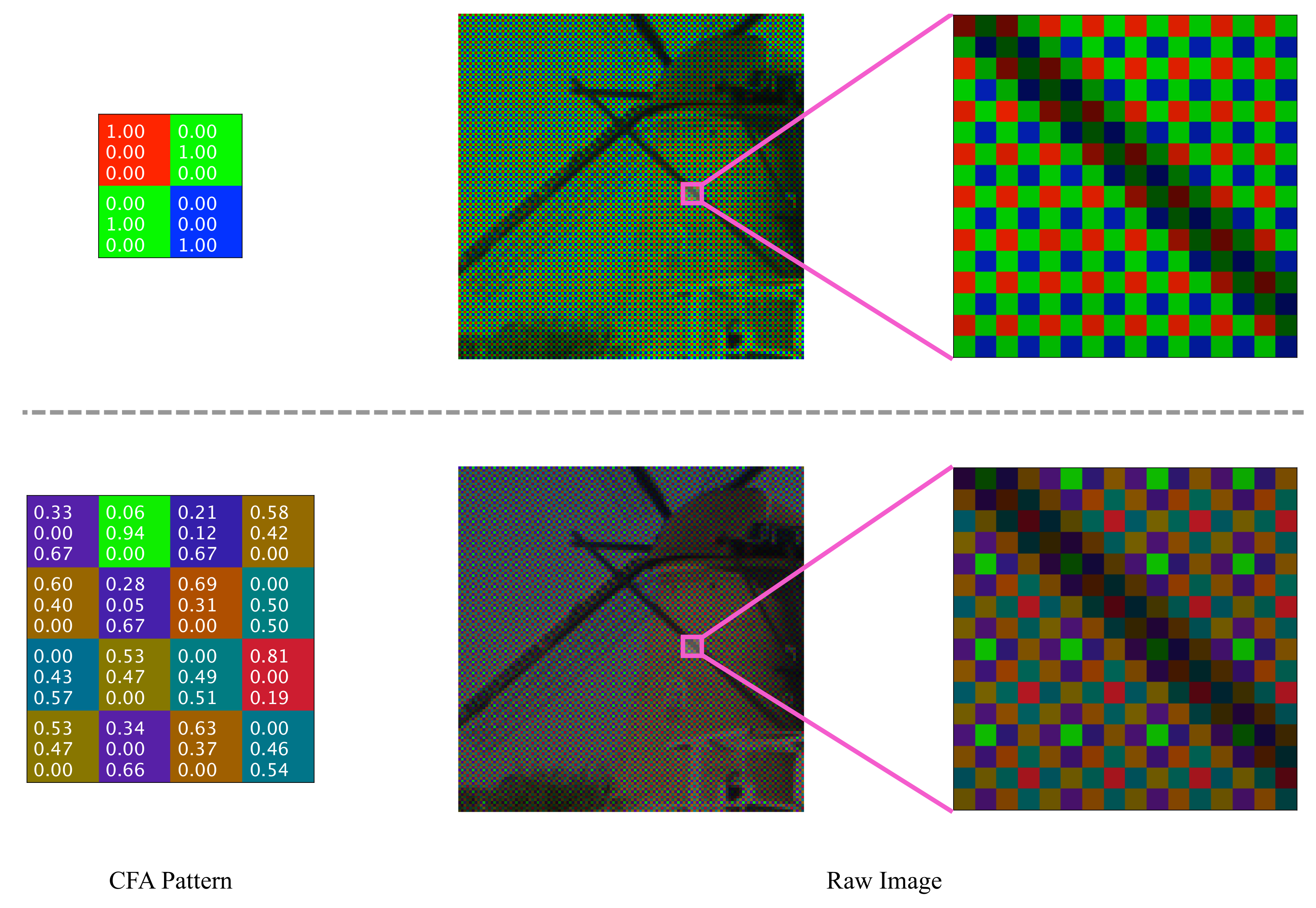
2.1. CFA Design
2.2. Demosaicing
2.3. Joint Optimization of CFA and Demosaicing
3. The Proposed Method
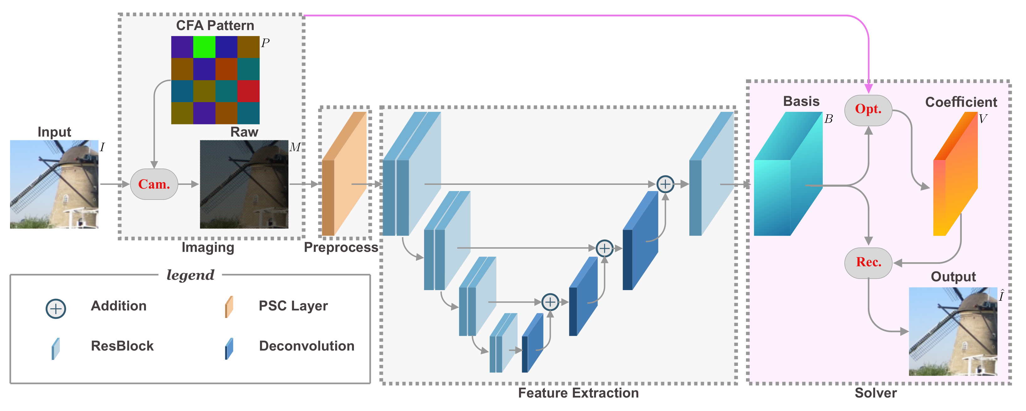
3.1. Overview
3.2. Model the Imaging Process
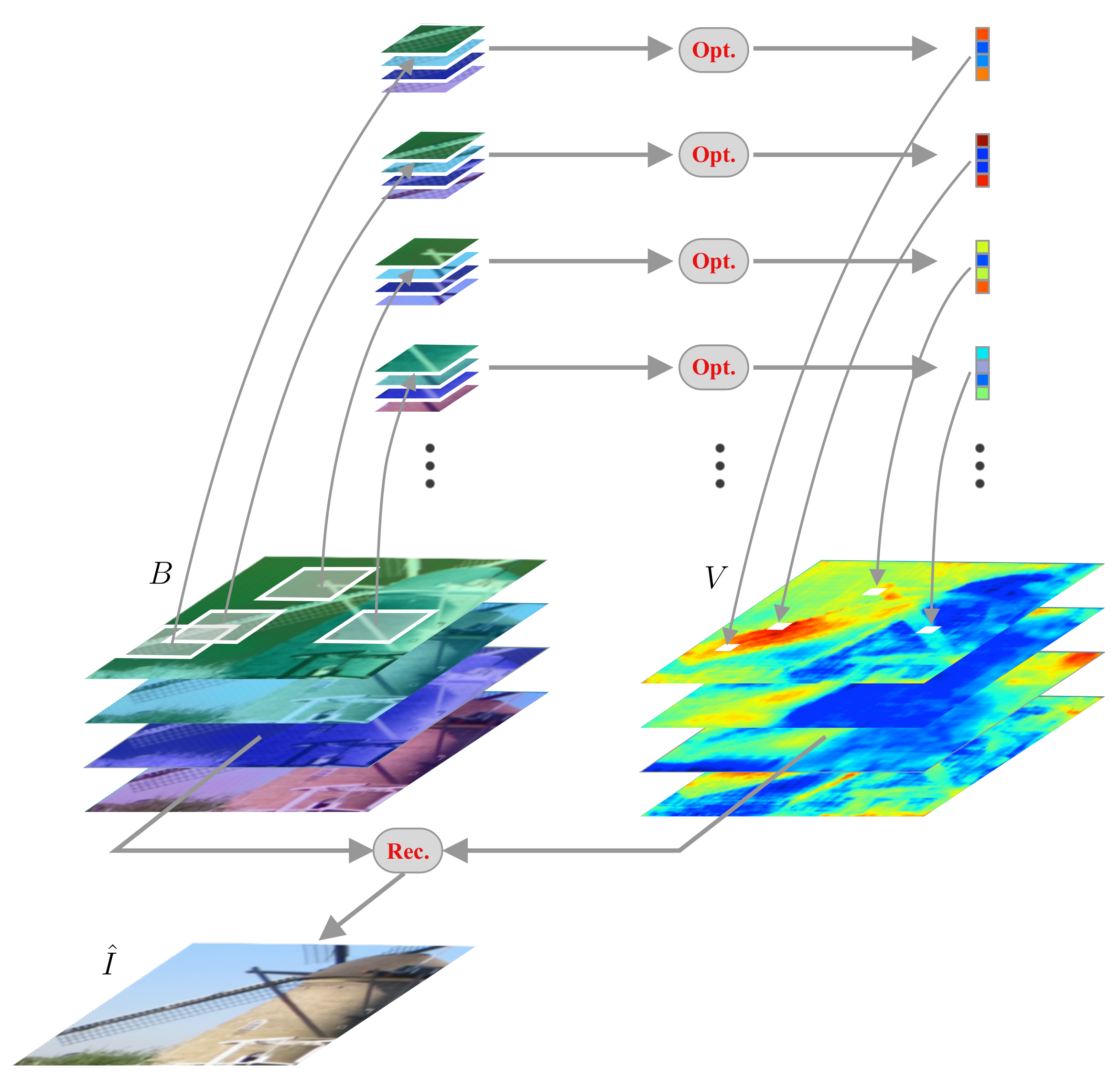
3.3. Differentiable Deep Restoration
3.3.1. Bases Generation Network with Sparse Data
3.3.2. Bases Generation Network with U-Net Structure
3.4. Joint Learning CFA and Demosaicing Network
3.5. Training Settings
4. Experiments
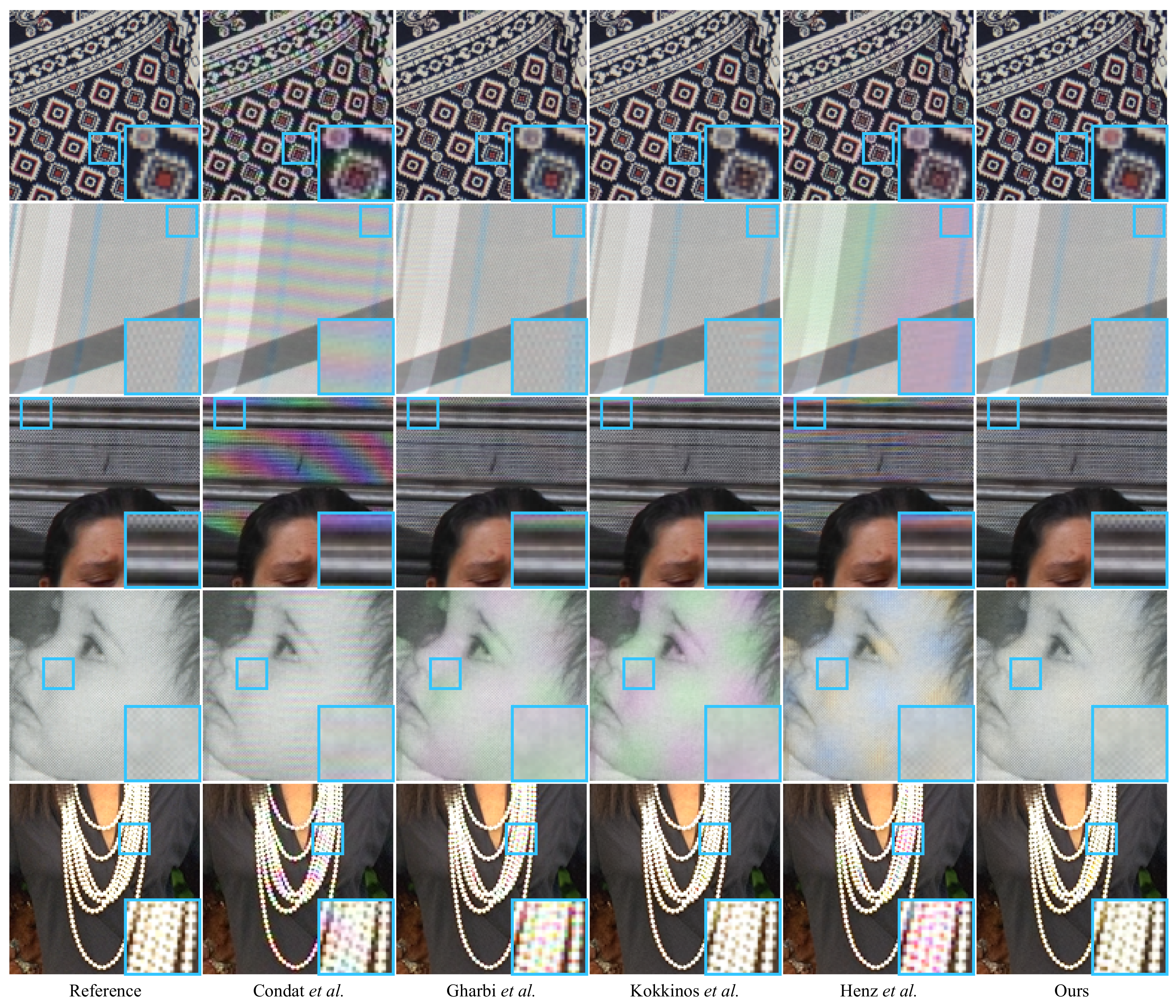
4.1. Reconstruction from Noise-Free Data
4.2. Ablation Studies
4.2.1. Sparse Data Processing and Optimization
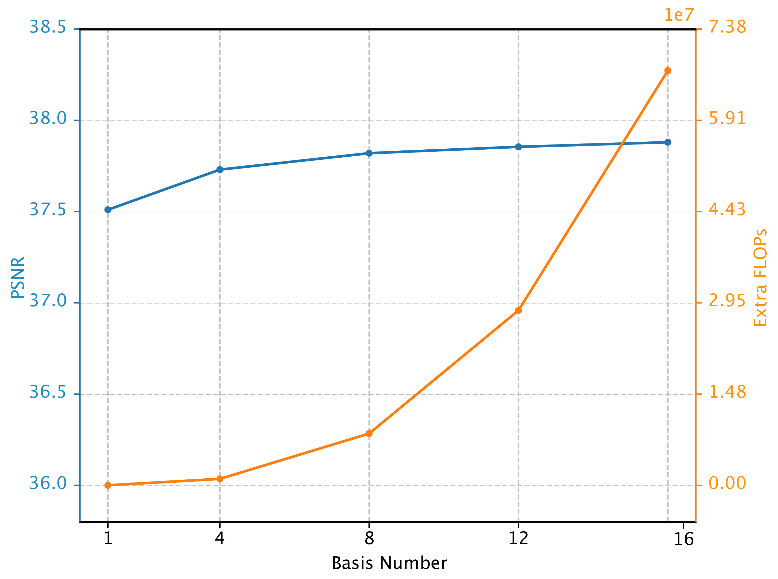
4.2.2. Different Basis Number
4.2.3. Effect of Patch-Based Optimization
4.3. Reconstruction from Noisy Data
4.4. Running Time Comparison
5. Conclusions
Author Contributions
Funding
Data Availability Statement
Conflicts of Interest
References
- Bayer, B.E. Color Imaging Array. U.S. Patent 3,971,065, 20 July 1976. [Google Scholar]
- Chakrabarti, A. Learning sensor multiplexing design through back-propagation. In Proceedings of the Advances in Neural Information Processing Systems, Barcelona, Spain, 5–10 December 2016; pp. 3081–3089. [Google Scholar]
- Henz, B.; Gastal, E.S.; Oliveira, M.M. Deep joint design of color filter arrays and demosaicing. Comput. Graph. Forum 2018, 37, 389–399. [Google Scholar] [CrossRef]
- Tang, C.; Yuan, L.; Tan, P. LSM: Learning Subspace Minimization for Low-level Vision. In Proceedings of the IEEE conference on computer vision and pattern recognition, Seattle, WA, USA, 13–19 June 2020. [Google Scholar]
- Zhang, K.; Zuo, W.; Gu, S.; Zhang, L. Learning deep CNN denoiser prior for image restoration. In Proceedings of the IEEE conference on computer vision and pattern recognition, Honolulu, HI, USA, 21–26 July 2017; pp. 3929–3938. [Google Scholar]
- Li, L.; Pan, J.; Lai, W.S.; Gao, C.; Sang, N.; Yang, M.H. Learning a discriminative prior for blind image deblurring. In Proceedings of the IEEE Conference on Computer Vision and Pattern Recognition, Salt Lake City, UT, USA, 18–23 June 2018; pp. 6616–6625. [Google Scholar]
- Tang, C.; Tan, P. BA-Net: Dense Bundle Adjustment Networks. In Proceedings of the International Conference on Learning Representations, New Orleans, LA, USA, 6–9 May 2019. [Google Scholar]
- Levin, A.; Lischinski, D.; Weiss, Y. A closed-form solution to natural image matting. IEEE Trans. Pattern Anal. Mach. Intell. 2007, 30, 228–242. [Google Scholar] [CrossRef]
- Gharbi, M.; Chaurasia, G.; Paris, S.; Durand, F. Deep joint demosaicking and denoising. ACM Trans. Graph. (TOG) 2016, 35, 191. [Google Scholar] [CrossRef]
- Franzen, R. Kodak Lossless True Color Image Suite. 1999. Volume 4. Available online: http://r0k.us/graphics/kodak (accessed on 13 June 2020).
- Zhang, L.; Wu, X.; Buades, A.; Li, X. Color demosaicking by local directional interpolation and nonlocal adaptive thresholding. J. Electron. Imaging 2011, 20, 023016. [Google Scholar]
- Yamagami, T.; Sasaki, T.; Suga, A. Image Signal Processing Apparatus Having a Color Filter with Offset Luminance Filter Elements. U.S. Patent 5,323,233, 21 June 1994. [Google Scholar]
- Zhu, W.; Parker, K.; Kriss, M.A. Color filter arrays based on mutually exclusive blue noise patterns. J. Vis. Commun. Image Represent. 1999, 10, 245–267. [Google Scholar] [CrossRef][Green Version]
- Condat, L. A new random color filter array with good spectral properties. In Proceedings of the 2009 16th IEEE International Conference on Image Processing (ICIP), Cairo, Egypt, 7–10 November 2009; pp. 1613–1616. [Google Scholar]
- Oh, P.; Lee, S.; Kang, M.G. Colorization-based RGB-white color interpolation using color filter array with randomly sampled pattern. Sensors 2017, 17, 1523. [Google Scholar] [CrossRef] [PubMed]
- Bai, C.; Li, J.; Lin, Z.; Yu, J.; Chen, Y.W. Penrose demosaicking. IEEE Trans. Image Process. 2015, 24, 1672–1684. [Google Scholar] [PubMed]
- Parmar, M.; Reeves, S.J. A perceptually based design methodology for color filter arrays [image reconstruction]. In Proceedings of the 2004 IEEE International Conference on Acoustics, Speech, and Signal Processing, Montreal, QC, Canada, 17–21 May 2004; Volume 3, p. iii–473. [Google Scholar]
- Lu, Y.M.; Vetterli, M. Optimal color filter array design: Quantitative conditions and an efficient search procedure. In Proceedings of the Digital Photography V, International Society for Optics and Photonics, San Jose, CA, USA, 5 June 2009; Volume 7250, p. 725009. [Google Scholar]
- Alleysson, D.; Susstrunk, S.; Hérault, J. Linear demosaicing inspired by the human visual system. IEEE Trans. Image Process. 2005, 14, 439–449. [Google Scholar]
- Hirakawa, K.; Wolfe, P.J. Spatio-spectral color filter array design for optimal image recovery. IEEE Trans. Image Process. 2008, 17, 1876–1890. [Google Scholar] [CrossRef] [PubMed]
- Hao, P.; Li, Y.; Lin, Z.; Dubois, E. A geometric method for optimal design of color filter arrays. IEEE Trans. Image Process. 2010, 20, 709–722. [Google Scholar]
- Bai, C.; Li, J.; Lin, Z.; Yu, J. Automatic design of color filter arrays in the frequency domain. IEEE Trans. Image Process. 2016, 25, 1793–1807. [Google Scholar] [CrossRef]
- Amba, P.; Dias, J.; Alleysson, D. Random color filter arrays are better than regular ones. In Proceedings of the Color and Imaging Conference, San Diego, CA, USA, 7–11 November 2016; Volume 2016, pp. 294–299. [Google Scholar]
- Amba, P.; Thomas, J.B.; Alleysson, D. N-LMMSE demosaicing for spectral filter arrays. J. Imaging Sci. Technol. 2017, 61, 40407–1. [Google Scholar] [CrossRef]
- Pei, S.C.; Tam, I.K. Effective color interpolation in CCD color filter arrays using signal correlation. IEEE Trans. Circuits Syst. Video Technol. 2003, 13, 503–513. [Google Scholar]
- Li, X. Demosaicing by successive approximation. IEEE Trans. Image Process. 2005, 14, 370–379. [Google Scholar]
- Li, X.; Orchard, M.T. New edge-directed interpolation. IEEE Trans. Image Process. 2001, 10, 1521–1527. [Google Scholar] [PubMed]
- Kakarala, R.; Baharav, Z. Adaptive demosaicing with the principal vector method. IEEE Trans. Consum. Electron. 2002, 48, 932–937. [Google Scholar] [CrossRef]
- Lu, W.; Tan, Y.P. Color filter array demosaicking: New method and performance measures. IEEE Trans. Image Process. 2003, 12, 1194–1210. [Google Scholar]
- Buades, A.; Coll, B.; Morel, J.M.; Sbert, C. Self-similarity driven color demosaicking. IEEE Trans. Image Process. 2009, 18, 1192–1202. [Google Scholar] [CrossRef]
- Mairal, J.; Elad, M.; Sapiro, G. Sparse representation for color image restoration. IEEE Trans. Image Process. 2007, 17, 53–69. [Google Scholar] [CrossRef]
- Ni, Z.; Ma, K.K.; Zeng, H.; Zhong, B. Color Image Demosaicing Using Progressive Collaborative Representation. IEEE Trans. Image Process. 2020, 29, 4952–4964. [Google Scholar] [CrossRef] [PubMed]
- Glotzbach, J.W.; Schafer, R.W.; Illgner, K. A method of color filter array interpolation with alias cancellation properties. In Proceedings of the 2001 International Conference on Image Processing (Cat. No. 01CH37205), Thessaloniki, Greece, 7–10 October 2001; Volume 1, pp. 141–144. [Google Scholar]
- Menon, D.; Calvagno, G. Color image demosaicking: An overview. Signal Process. Image Commun. 2011, 26, 518–533. [Google Scholar] [CrossRef]
- Tan, R.; Zhang, K.; Zuo, W.; Zhang, L. Color image demosaicking via deep residual learning. In Proceedings of the 2017 IEEE International Conference on Multimedia and Expo (ICME), Hong Kong, China, 10–14 July 2017; pp. 793–798. [Google Scholar]
- Cui, K.; Jin, Z.; Steinbach, E. Color image demosaicking using a 3-stage convolutional neural network structure. In Proceedings of the 2018 25th IEEE International Conference on Image Processing (ICIP), Athens, Greece, 7–10 October 2018; pp. 2177–2181. [Google Scholar]
- Huang, T.; Wu, F.F.; Dong, W.; Shi, G.; Li, X. Lightweight Deep Residue Learning for Joint Color Image Demosaicking and Denoising. In Proceedings of the 2018 24th International Conference on Pattern Recognition (ICPR), Beijing, China, 20–24 August 2018; pp. 127–132. [Google Scholar]
- Liu, L.; Jia, X.; Liu, J.; Tian, Q. Joint demosaicing and denoising with self guidance. In Proceedings of the IEEE/CVF Conference on Computer Vision and Pattern Recognition, Seattle, WA, USA, 13–19 June 2020; pp. 2240–2249. [Google Scholar]
- Kokkinos, F.; Lefkimmiatis, S. Deep image demosaicking using a cascade of convolutional residual denoising networks. In Proceedings of the European Conference on Computer Vision (ECCV), Munich, Germany, 8–14 September 2018; pp. 303–319. [Google Scholar]
- Kokkinos, F.; Lefkimmiatis, S. Iterative Joint Image Demosaicking and Denoising using a Residual Denoising Network. IEEE Trans. Image Process. 2019. [Google Scholar] [CrossRef]
- Bean, J.J. Cyan-Magenta-Yellow-Blue Color Filter Array. U.S. Patent 6,628,331, 30 September 2003. [Google Scholar]
- Lapray, P.J.; Wang, X.; Thomas, J.B.; Gouton, P. Multispectral filter arrays: Recent advances and practical implementation. Sensors 2014, 14, 21626–21659. [Google Scholar] [CrossRef]
- Ronneberger, O.; Fischer, P.; Brox, T. U-net: Convolutional networks for biomedical image segmentation. In Proceedings of the International Conference on Medical image computing and computer-assisted intervention, Munich, Germany, 5–9 October 2015; Springer: Berlin/Heidelberg, Germany, 2015; pp. 234–241. [Google Scholar]
- Long, J.; Shelhamer, E.; Darrell, T. Fully convolutional networks for semantic segmentation. In Proceedings of the IEEE Conference on Computer Vision and Pattern Recognition, Boston, MA, USA, 7–12 June 2015; pp. 3431–3440. [Google Scholar]
- He, K.; Zhang, X.; Ren, S.; Sun, J. Deep residual learning for image recognition. In Proceedings of the IEEE conference on computer vision and pattern recognition, Las Vegas, NV, USA, 27–30 June 2016; pp. 770–778. [Google Scholar]
- Ioffe, S.; Szegedy, C. Batch normalization: Accelerating deep network training by reducing internal covariate shift. arXiv 2015, arXiv:1502.03167. [Google Scholar]
- Kingma, D.P.; Ba, J. Adam: A method for stochastic optimization. arXiv 2014, arXiv:1412.6980. [Google Scholar]
- Wang, Z.; Bovik, A.C.; Sheikh, H.R.; Simoncelli, E.P. Image quality assessment: From error visibility to structural similarity. IEEE Trans. Image Process. 2004, 13, 600–612. [Google Scholar] [CrossRef] [PubMed]
- Li, J.; Bai, C.; Lin, Z.; Yu, J. Optimized color filter arrays for sparse representation-based demosaicking. IEEE Trans. Image Process. 2017, 26, 2381–2393. [Google Scholar] [CrossRef] [PubMed]
- Chakrabarti, A.; Freeman, W.T.; Zickler, T. Rethinking color cameras. In Proceedings of the 2014 IEEE International Conference on Computational Photography (ICCP), Santa Clara, CA, USA, 2–4 May 2014; pp. 1–8. [Google Scholar]
- Condat, L.; Mosaddegh, S. Joint demosaicking and denoising by total variation minimization. In Proceedings of the 2012 19th IEEE International Conference on Image Processing, Orlando, FL, USA, 30 September–3 October 2012; pp. 2781–2784. [Google Scholar]
- Condat, L. A new color filter array with optimal properties for noiseless and noisy color image acquisition. IEEE Trans. Image Process. 2011, 20, 2200–2210. [Google Scholar] [CrossRef] [PubMed]
- Jeon, G.; Dubois, E. Demosaicking of noisy Bayer-sampled color images with least-squares luma-chroma demultiplexing and noise level estimation. IEEE Trans. Image Process. 2012, 22, 146–156. [Google Scholar] [CrossRef]
- Ye, W.; Ma, K.K. Color image demosaicing using iterative residual interpolation. IEEE Trans. Image Process. 2015, 24, 5879–5891. [Google Scholar] [CrossRef] [PubMed]


| Demosaic | Kodak | McMaster | vdp | moiré | ||||
|---|---|---|---|---|---|---|---|---|
| (Bayer CFA) | (24 images) | (18 images) | (1000 images) | (1000 images) | ||||
| PSNR | SSIM | PSNR | SSIM | PSNR | SSIM | PSNR | SSIM | |
| Bilinear | 29.26 | 0.881 | 30.81 | 0.922 | 23.77 | 0.806 | 25.27 | 0.820 |
| Condat et al. [51] | 34.81 | 0.954 | 30.20 | 0.861 | 27.34 | 0.886 | 29.90 | 0.883 |
| Tan et al. [35] | 41.98 | 0.988 | 38.94 | 0.969 | 32.99 | 0.955 | 34.28 | 0.930 |
| Gharbi et al. [9] | 41.50 | 0.987 | 39.14 | 0.971 | 33.95 | 0.973 | 36.62 | 0.960 |
| Cui et al. [36] | 42.18 | 0.988 | 39.33 | 0.972 | 33.23 | 0.960 | 34.74 | 0.934 |
| Huang et al. [37] | 42.34 | 0.989 | 39.10 | 0.970 | 33.46 | 0.959 | 34.99 | 0.935 |
| Henz et al. [3] | 41.93 | 0.988 | 39.51 | 0.972 | 34.30 | 0.973 | 36.41 | 0.956 |
| Kokkinos et al. [40] | 41.65 | 0.989 | 39.51 | 0.971 | 34.46 | 0.966 | 36.93 | 0.956 |
| Ni et al. [32] | 40.36 | 0.986 | 38.11 | 0.967 | 31.54 | 0.943 | 32.95 | 0.926 |
| Our 2 × 2 Bayer | 42.49 | 0.989 | 39.76 | 0.972 | 35.04 | 0.977 | 37.54 | 0.952 |
| (Non-Bayer CFA) | Kodak | McMaster | vdp | moiré | ||||
| PSNR | SSIM | PSNR | SSIM | PSNR | SSIM | PSNR | SSIM | |
| Chakrabarti et al. [50] | 33.51 | 0.962 | 30.95 | 0.921 | 25.91 | 0.897 | 28.77 | 0.910 |
| Condat et al. [52] | 39.96 | 0.986 | 33.88 | 0.931 | 30.04 | 0.934 | 33.33 | 0.927 |
| Hao et al. [21] | 39.42 | — | — | — | — | — | — | — |
| Bai et al. [22] | 40.24 | — | — | — | — | — | — | — |
| Hirakawa et al. [20] | 40.36 | — | — | — | — | — | — | — |
| Li et al. [49] | 41.59 | — | — | — | — | — | — | — |
| (Joint-Learned CFA) | Kodak | McMaster | vdp | moiré | ||||
| PSNR | SSIM | PSNR | SSIM | PSNR | SSIM | PSNR | SSIM | |
| Chakrabarti et al. [2] | 31.35 | 0.920 | 28.39 | 0.835 | 24.98 | 0.824 | 27.91 | 0.845 |
| Henz et al. [3] | 43.13 | 0.991 | 40.18 | 0.976 | 35.17 | 0.977 | 37.70 | 0.961 |
| Our Learned 4 × 4 | 43.87 | 0.992 | 40.60 | 0.976 | 36.14 | 0.981 | 39.28 | 0.967 |
| Preprocessing | Optimization | Basis Number | PSNR |
|---|---|---|---|
| Rearranging | No | — | 36.68 |
| Interpolation | No | — | 36.79 |
| PSC | No | — | 36.90 |
| PSC | Global | 4 | 37.61 |
| PSC | Global | 8 | 37.64 |
| PSC | Global | 12 | 37.67 |
| PSC | Global | 16 | 37.43 |
| PSC | Local | 4 | 37.71 |
Publisher’s Note: MDPI stays neutral with regard to jurisdictional claims in published maps and institutional affiliations. |
© 2021 by the authors. Licensee MDPI, Basel, Switzerland. This article is an open access article distributed under the terms and conditions of the Creative Commons Attribution (CC BY) license (http://creativecommons.org/licenses/by/4.0/).
Share and Cite
Tang, J.; Li, J.; Tan, P. Demosaicing by Differentiable Deep Restoration. Appl. Sci. 2021, 11, 1649. https://doi.org/10.3390/app11041649
Tang J, Li J, Tan P. Demosaicing by Differentiable Deep Restoration. Applied Sciences. 2021; 11(4):1649. https://doi.org/10.3390/app11041649
Chicago/Turabian StyleTang, Jie, Jian Li, and Ping Tan. 2021. "Demosaicing by Differentiable Deep Restoration" Applied Sciences 11, no. 4: 1649. https://doi.org/10.3390/app11041649
APA StyleTang, J., Li, J., & Tan, P. (2021). Demosaicing by Differentiable Deep Restoration. Applied Sciences, 11(4), 1649. https://doi.org/10.3390/app11041649