Article

Integrated Tolerance and Fixture Layout Design for Compliant Sheet Metal Assemblies

by
Abolfazl Rezaei Aderiani
1,*,
Martin Hallmann
2,
Kristina Wärmefjord
1,
Benjamin Schleich
2,
Rikard Söderberg
1 and
Sandro Wartzack
2
1
Department of Industrial and Materials Science, Chalmers University of Technology, 41296 Gothenburg, Sweden
2
Engineering Design, Friedrich-Alexander-Universität Erlangen-Nürnberg, 91058 Erlangen, Germany
*
Author to whom correspondence should be addressed.
Appl. Sci. 2021, 11(4), 1646; https://doi.org/10.3390/app11041646
Submission received: 15 January 2021 / Revised: 8 February 2021 / Accepted: 9 February 2021 / Published: 11 February 2021
(This article belongs to the Special Issue Mechanical Tolerance Analysis in the Era of Industry 4.0)

Abstract

:

Featured Application

This paper addresses an industrial problem, namely geometrical variations in assemblies. Accordingly, the potential application of the findings are in the design and production of the compliant assemblies, particularly spot-welded assemblies in the automotive industries.

Abstract

Part tolerances and fixture layouts are two pivotal factors in the geometrical quality of a compliant assembly. The independent design and optimization of these factors for compliant assemblies have been thoroughly studied. However, this paper presents the dependency of these factors and, consequently, the demand for an integrated design of them. A method is developed in order to address this issue by utilizing compliant variation simulation tools and evolutionary optimization algorithms. Thereby, integrated and non-integrated optimization of the tolerances and fixture layouts are conducted for an industrial sample case. The objective of this optimization is defined as minimizing the production cost while fulfilling the geometrical requirements. The results evidence the superiority of the integrated approach to the non-integrated in terms of the production cost and geometrical quality of the assemblies.

1. Introduction

Geometrical variation is an inevitable consequence of the mass production of physical products. The variation is directly related to the quality of a product, and it can result in added costs to the production of a product [1]. Moreover, geometrical variation commonly affects the functionality of the product and its aesthetical aspects [2].
Geometrical tolerances and the fixture layout are two main factors in defining the geometrical quality of sheet metal assemblies. Accordingly, determining their optimal design is crucial in the development of these products. The optimization of each factor separately has been comprehensively developed in previous studies. However, the integrated optimal design of these factors is a research gap that this paper aims to address. The presented method leverages from the opportunity that is provided by available data in the new industrial era, i.e., Industry 4.0 [3]. These data include the non-nominal geometry of produced parts, available measurement data of produced parts, and predictability of the deformed forms that result from different production processes.
Section 1.1 defines the tolerance–cost optimization and reviews the previous studies in this regard. Afterward, Section 1.2 presents a brief review of fixture layout optimization studies. The method presented in this paper utilizes compliant variation simulations in order to determine the geometrical quality of the assemblies. Hence, Section 1.3 elucidates the state of the art in these simulations. Section 1.4 clarifies the research gap and an outline of the paper.

1.1. Tolerance-Cost Optimization

Managing uncertainty is a key activity in product development to realize products with high reliability, robustness, and safety [4,5]. In this regard, tolerancing aims to assure product quality, e.g., functionality or aesthetics, by managing and limiting the unavoidable geometric part variations caused by manufacturing uncertainty [4,6]. Tolerance design, which corresponds to the last step in a robust product design [1], consists of three main tasks, viz. tolerance specification, tolerance allocation, and tolerance analysis [7]. While tolerance types and references are chosen for the functional relevant geometry elements in tolerance specification, tolerance allocation is used to assign suitable tolerance values to them [7]. In the early years of tolerancing, experience, handbooks or best practices [8], graphical and simple analytical approaches, such as equal or proportional scaling [9,10], as well as the repetitive application of tolerance and sensitivity analysis [11], could meet the former requirements [12,13].
However, the steadily increasing cost and quality pressure required the development of more sophisticated approaches to automatically find the combination of tolerance values that lead to minimum costs, but can also assure high product quality [12,13]. Tolerance-cost optimization—also known under the terms optimal/least-cost tolerance allocation/design/synthesis—accelerates the usually manual, trial-and-error based search by turning the task into a mathematical optimization problem in order to find the optimal compromise between cost and quality [12]. In the beginning, its applicability was mainly limited by the low computing powers and the lack of powerful optimization algorithms [12]. The development of soft-computing, nature-inspired meta-heuristic algorithms, in combination with the significantly increased computer technology, has finally paved the way for its practical application to complex engineering systems [12,13].
At the same time, the general idea of concurrent and simultaneous engineering has lead to a joint consideration of the previously separated optimization-based tolerance allocation methods from the design and manufacturing [12,13]. As a consequence, design-driven approaches have successively adopted additional manufacturing aspects, which lead to a shift to a process-oriented tolerance allocation [12,14].
In this regard, the research scope mainly depends on the addressed type of assembly process [12,15]. The total variation of assemblies, where the parts are located and fixed through part-to-part mating surfaces, is mostly influenced by the individual geometrical part variations [15,16]. Further cost aspects, such as quality loss, including tool degradation and maintenance planning [15,17,18] and environmental costs [19], can additionally be considered in tolerance-cost optimization. Research in the field of process-oriented tolerancing summarily shows that the joining technique itself, the assembly and the fixture layout, and its tolerances have a significant impact on the results of optimal tolerance allocation.

1.2. Assembly Fixture Layout Optimization

A fixture may be used for different applications in production. Machining fixtures are primarily utilized to withstand against displacement or plastic deformations, due to the machining forces [20]. However, in the design of assembly fixtures, the principle design objective is to minimize the sensitivity of the assembly to variation of the rigid parts [21]. The part variations can be magnified or lessened in the assemblies, depending on the assembly fixture layout.
The common types of locators are four-way-pins, two-way-pins, and clamps. The four-way-pins are commonly positioned in a hole in the part and the two-way-pins in a slot. Accordingly, four-ways-pins and two-ways-pins can be referred to as a hole and slot, respectively. A hole locks two in-plane translations of the part. A slot locks one in-plane translation, and a clamping unit locks the translation of the part normal to the clamping surface. If a hole or a slot is clamped, their translation will also be locked in the normal direction. Figure 1 depicts an example of a sheet metal part that is locked through a hole, a slot, and three clamping units.
The assembly is considered to be non-rigid or compliant if the parts deform during the assembly procedure or after releasing the clamps (i.e., spring-back occurs). The studies regarding assembly fixture layout optimization can be divided into two categories of fixtures for rigid assemblies and fixtures for compliant assemblies. A difference between these two categories is the method utilized to determine the relationship between the part variation and assembly variation.
In rigid assemblies, the effects of part variations in the locating areas are identical to the effects of locator variations in these areas. Hence, the sensitivity of a rigid assembly to a fixture layout can be determined by disturbing its locating positions and evaluating the consequences on the assembly [23]. Jin et al. [24] have developed a state-space model that is based on this technique in order to determine the relationship between the variation of KPCs and variation in the locating points. This model and its other variants are utilized in the fixture layout optimization of rigid assemblies by most of the studies [25,26,27,28,29,30]. Most of these studies have utilized state-space modeling to optimize the fixture layouts of all assembly stations simultaneously in multi-station assemblies.
In compliant assemblies, the parts may be over-constrained by a fixture. A typical locating layout of a compliant part in an assembly fixture is an N-2-1 (N > 3) layout. In this layout, the number of holes and slots are the same as the numbers for rigid parts (i.e., one hole and one slot in each part), but the number of clamping units differs. Consequently, the number of additional clamps is a design parameter in compliant fixture layout optimization that does not exist in rigid fixture layout optimization.
The relation between the assembly variation and variation of parts is more complicated in compliant assemblies than rigid assemblies. This relation is commonly determined through several finite element simulations that are elaborated in Section 1.3. Contrary to the rigid assemblies, the fixture layout of compliant assemblies is typically conducted for one station.
The design parameters in most of the studies regarding fixture layout optimization of compliant assemblies are the coordinates of one or several clamping units in a part [31,32,33,34,35,36]. Xing et al. [37] utilized the location of the clamping units as the node number of the part and not their coordinates. Aderiani et al. [38] considered the location of holes, slots, clamping units, in addition to their types and the number of additional clamps as the design parameters for the optimization.

1.3. Compliant Variation Simulations

The parts of a compliant assembly may deform during the assembly process and spring-back can occur. Therefore, finite element analysis is utilized in order to determine the deviations of these assemblies from their nominal geometry (i.e., the geometry after spring-back). The assembly process of spot-welded sheet metal assemblies can be divided into four steps [39]. The first step is to position the non-ideal parts in the assembly fixture. The second step is to clamp these parts into their nominal shapes. Subsequently, the parts are welded in the third step, and the clamps are released in the fourth step.
Deviations of the parts from their nominal geometries are represented by [ D 1 ] . Therefore, the clamping forces (in the second step) can be determined by Equation (1). In this equation, [ K 1 ] and [ F c 1 ] are the stiffness matrix of the parts before assembly and the clamping forces, respectively.
[ F c 1 ] = [ K 1 ] [ D 1 ]
The stiffness matrix of parts after welding can be determined by merging the nodes of parts in the welding areas. This matrix is indicated by [ K 2 ] . Supposing that the welding does not imply additional deformations, the clamping forces before and after welding are equal ( [ F c 1 ] = [ F c 2 ] ). Thereby, the second FE simulations can determine the deviations of the assembly after releasing the clamps, [ D 2 ] , through Equation (2).
[ D 2 ] = [ K 2 ] 1 [ F c 2 ] = [ K 2 ] 1 [ F c 1 ] = [ K 2 ] 1 [ K 1 ] [ D 1 ]
The distribution of deviation of the assembly can be determined by simulating thousands of random input deviations of the parts. FE simulations may have a relatively high calculation cost. Consequently, determining the variation of thousands of assemblies will be computationally expensive. Li and Hu [39] have addressed this issue by assuming a linear relation between the deviations of the assemblies and parts. Thereby, a sensitivity matrix ( [ S ] ) is determined by conducting two FE simulations. Hence, Equation (3) can determine the assembly deviations for every part deviation. This method is known as the method of influence coefficients (MIC).
[ D 2 ] = [ S ] [ D 1 ]
Dahlström et al. [40] demonstrated that this method may lead to severe errors in the results, because the contacts between the parts are not considered. They proposed a new MIC, in which contact modeling is considered, but it is not linear. The reason for non-linearity is that the contacts are dependent on the deviation of the parts, and these deviations vary for each part. Consequently, the stiffness matrix should be updated in every iteration of the simulations. Wärmefjord et al. [41] improved this method by developing a method for automatically detecting these contacts in each iteration. Lindau et al. [42] further improved the efficiency of the variations by presenting a quadric optimization to solve the contact equations.
The variation simulation techniques have become more sophisticated by considering the effects of heat [43], non-linearity of materials [44], and welding sequences [45,46]. Several commercial programs have been developed to implement these techniques in CAD models for practical uses.

1.4. Scope of the Paper

The fixture layout and part tolerances are crucial factors in determining the quality and cost of productions, particularly in compliant sheet metal assemblies. Accordingly, numerous studies have addressed the optimization of these factors in order to minimize the production cost or maximize the quality. However, the optimal design of each factor is dependent on the other factor. Consequently, independent optimization of each factor may not result in the maximum quality and the minimum cost. Therefore, the optimal integrated design of the tolerances and fixture layouts, particularly for compliant assemblies, comprises the research gap that this paper aims to address.
Section 2 classifies the optimization problem by clarifying the objectives, design parameters, and constraints. Subsequently, Section 3 elaborates the optimization method that was developed to address the problem. The results of applying the developed method on an industrial sample case and discussions on them are presented in Section 4 and Section 5, respectively.

2. Problem Description

This study aims to develop a method for determining the optimal tolerances and fixture layout of the compliant assemblies. Hence, this problem is elucidated in this section by introducing its design parameters in Section 2.1, defining its objective function in Section 2.2 and clarifying the constraints in Section 2.3.

2.1. Design Parameters

The main factors that are to be optimized in this study are the part tolerances and the fixture layout. Accordingly, the design parameters that control each of these factors are clarified separately.

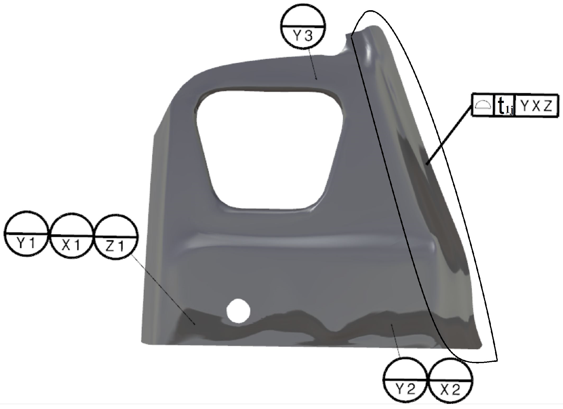
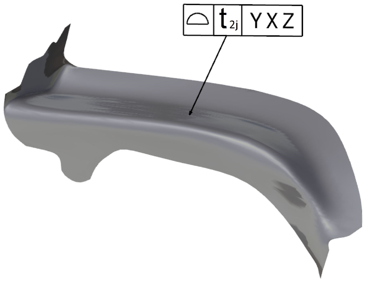
2.1.1. Design Parameters of Tolerances

There are numerous production restrains that should be considered in the design of tolerances for sheet metal assemblies in practice. These parts, particularly in a car body, are produced by forming, stamping, and bending. Each of these processes adds several limits to the accuracy and precision with which the parts can be produced. Accordingly, the design domain in which the tolerances can be defined is restricted to a limited number of production scenarios for each part. Each scenario results from producing the part with specific tolerances of each process, the sequence of processes, and the geometry of the part. Supposing that there are T i different tolerances resulting from each production scenario of part i, each tolerance is indicated by t i j ( i , j     Z + , 1   <   i     m , 1   <   j     T i ). (see Table 1). The number of parts in the assembly is represented by m.
The design parameter that defines which t i j to use for producing each part is defined as x i j ( x i j     { 0 , 1 } ), where x i j = 1 indicates the scenario j is utilized to produce part i. Therefore, only one x i j for part i can be one and the rest are zero. Accordingly, defining which x i j is one for part number i means defining with which production process this part is produced, i.e., the tolerances of part i ( t i j ). New dimensions can be added to the x, i.e., x i j k if a part has more than one tolerance and the value of the tolerances can independently vary.

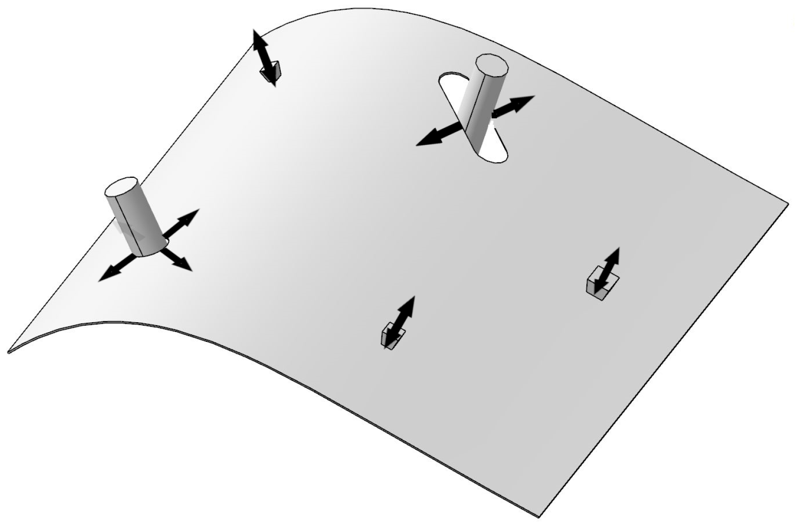
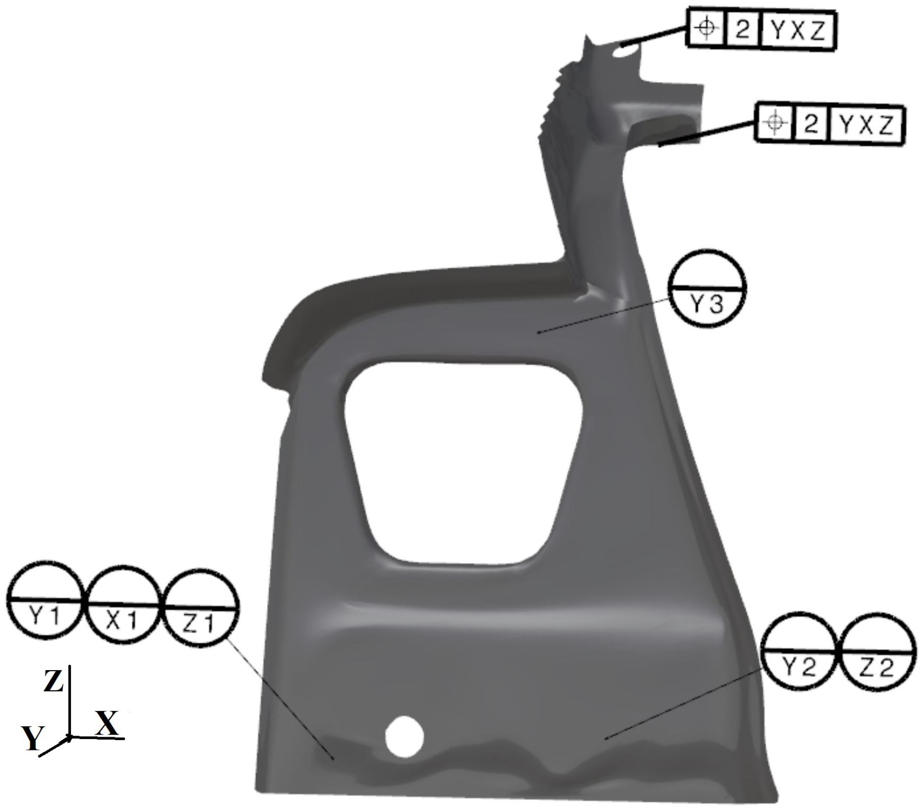
2.1.2. Design Parameters of Fixture Layouts

A fixture layout is defined by the location and the number of its locators on each part of the assembly. It is assumed that each part has a N 2 1 , ( N 3 ) locating layout. Therefore, each part has one hole and one slot, and the optimization algorithm defines the optimal number of clamps (N). Hence, the design parameters of the fixture layout are the number of additional clamps, the location of holes, slots, and clamps, and the slot directions. A clamping unit can be positioned where a hole or slot is positioned. The hole or slot is clamped in this situation.
The parameters to define the location of the locators can be either the coordinates of them or a node number. The later choice reduces the optimization size and complexities of the problem [37,38]. Hence, the node number is used as the parameter to define the optimal location of each locator. Because this approach was developed by Aderiani et al. [38] to define the design parameters of fixture layouts, the same parameters for the fixture layout are employed in this paper. These parameters are listed in Table 2, and they are introduced in this section.
Not all areas of a part can be the location of a locator. Areas that are close to edges, bends, and areas that are not practically accessible cannot be the position of a locator. Therefore, the node numbers that can be utilized to be the position of a locator can be filtered, and the rest can be removed from the design space. Moreover, if the size of elements in each part is significantly smaller than the size of the part, changing the position of a locator from a node to the next node may not affect the results significantly. Therefore, to simplify the optimization problem, the feasible areas of each part can be divided into some smaller areas, and one node from each area (a node that is approximately in the center of the area) is considered to be the representative node of that area [38].
After discritizing the feasible areas and selecting the candidate node, each node of part i is represented by k ( k Z + , 1 k n ), where n is the number of all candidate nodes in part i. The parameter α i k is introduced as a parameter to indicate whether the node k in part i is clamped. Accordingly, α i k = 1 indicates the node k of part i is clamped and α i k = 0 demonstrates that the node is not clamped.
Each part has one hole and one slot. Therefore, two parameters are utilized to indicate the location (the node number) of the hole and the slot in each part. These parameters are β i , 1 , and β i , 2 ( ( β i , 1 , β i , 2 k ) ) for the hole and slot, respectively. θ i ( 0 θ i < 180 ) is also introduced to define the slot direction in part i. This parameter indicates the angle between the in-plane locking direction of the slot in part i and a fix arbitrary direction in the same plane.

2.2. Objectives

Part tolerances and fixture layouts directly influence the production costs and geometrical quality of the assemblies. Depending on the application, both or one of these parameters can be considered as the objective of the optimization. The minimal geometrical quality of the assembly is commonly defined through tolerances on the KPCs of the assembly. Thereby, the objective is defined as minimizing the cost of part production while fulfilling the geometrical requirements of the assemblies.
Each production scenario is associated with a production cost. The cost is commonly higher for the scenarios in which the produced parts have a greater geometrical quality. Supposing that the scenario j for part i costs c i j , the total cost of production can be determined by Equation (4).
C = i = 1 m j = 1 T i c i j x i j
The minimal geometrical requirement is a problem constraint. However, this problem can be added to the objective function as a penalty. The penalty function should increase the value of the objective function when the geometrical quality is lower than the required quality and it does not add anything when it is higher.
The deviation of each part may differ from the others in KPCs during mass production. Therefore, a statistical measurement is commonly utilized in order to evaluate whether the minimal requirements in KPCs are satisfied. In cases where the deviations are normally distributed, the process capability index ( C p k ) can be utilized to evaluate the geometrical quality. Equation (5) represents the definitions of this parameter.
C p k = min { U L d ¯ 3 σ , d ¯ L L 3 σ }
In this equation, U L and L L represent the upper and lower limits of the KPC, respectively. The parameter σ is the standard deviation of the KPC and d ¯ is the mean value of its deviations. If the KPCs are defined by geometrical tolerances (as they are in the sample case utilized in this paper), the magnitude of deviation is utilized for evaluation, which cannot be negative. Consequently, the distribution of the deviation is not normal, and Equation (5) cannot be utilized to evaluate it. A more general definition of capability index, which is referred to as Clement’s method [47], is utilized to address this issue. Equation (6) represents this definition. In this equation, ζ 0.99865 and ζ 0.00135 are the upper and lower 0.135th percentiles of the distribution, respectively, and ζ 0.5 is the median of the distribution instead of its mean. Because there is no lower limit in the magnitude of the deviation, C p u is utilized in this paper to measure the geometrical quality.
C p k = min { U L ζ 0.5 ζ 0.99865 ζ 0.5 , ζ 0.5 L L ζ 0.5 ζ 0.00135 } = min { C p u , C p l }
A C p u 1.67 indicates 99.99% of the produced assemblies satisfy the defined limits of KPCs (if the 0.001th percentile is used in the formulation, C p u 1 indicates the same quality). Hence, the required geometrical is defined as having C p u 1.67 for each KPC. If this requirement is not satisfied, then a penalty relative to its value will be considered as the penalty. Equation (7) represents this penalty function.
p ( C p u ) = 0 C p u 1.67 1.67 C p u C p u < 1.67

2.3. Constraints

The feasible values of each parameter, as defined in Section 2.1, are the constraints that should be considered in the optimization. Moreover, the locating layout must constrain the rigid body motions for each part. This constraint can be controlled by evaluating the rank of its Jacobian matrix [48], as presented in Equation (8). In this equation, the coordinates of locator l are presented by c l , the number of locators of each part by L and its locking direction is indicated by n l . Thereby, the constraint to avoid rigid body motions is J 6 for each part.
J = ( c 1 × n 1 ) T n 1 T ( c 2 × n 2 ) T n 2 T ( c L × n L ) T n L T
Another constraint to consider is that the locations of holes and slots cannot be in the same node. Equation (9) presents this constraint.
β i , 1 β i , 2

3. Optimization Method

The problem that is described in Section 2 is an optimization problem. Section 3.1 elaborates the formulation of this problem. Subsequently, Section 3.2 establishes an optimization algorithm to solve this problem.

3.1. Optimization Problem

Equation (10) presents the mathematical formulation of the optimization problem. The production cost in the objective function is normalized (relative to the maximum production cost) in order to make the function independent of the production cost magnitude. Moreover, the penalty of violating the minimal geometrical quality is the summation of the penalty of all KPCs (the number of KPCs in the assembly is represented by K). This penalty is defined, so that it is greater than the cost (See Equation (7)). Therefore, the objective value is lower for the most expensive solution that passes the minimal geometrical quality than the cheapest solution that does not pass the minimal geometrical quality. Thereby, the solutions that do not satisfy the geometrical quality requirements cannot be better than those that satisfy them, no matter how cheaper their production cost is. The constraints that are defined in this optimization problem should be valid for all parts (i.e., for every i).
min f ( x , α , β 1 , β 2 , θ ) = C C m a x + k = 1 K p ( C p u k )
Subject to:
j = 1 T i x i j = 1
x i j { 0 , 1 }
α i k { 0 , 1 }
β i , 1 , β i , 2 { 1 , 2 , , n }
β i , 1 β i , 2
0 θ p < 180 °
r a n k ( J ) 6
The objective function of this optimization problem is a black-box function, in which thousand random simulations are conducted in each function evaluation. The proper optimization algorithms to address these types of problems are meta-heuristic optimization algorithms. Among these algorithms, Genetic Algorithms (GA) are often used in engineering-based optimization tools and a numerous varieties of them have been developed for different applications. Hence, this paper utilizes a multinary GA to solve the optimization problem presented.

3.2. Optimization Algorithm

A GA is an evolutionary optimization algorithm meaning the solutions are evolved during a certain number of iterations. The utilized GA algorithm in this paper is denoted in Algorithm 1. Commonly, a population of random solutions is generated to start the optimization procedure. Subsequently, each solution receives a fitness value that is proportional to the value of the objective function for it. Afterward, new solutions are generated through genetic operations, including crossover and mutation. The new solutions with greater fitness values will substitute solutions with lower fitness values. This procedure will continue until the convergence criteria are satisfied.
The value of x i j is zero for all js, except one for each part. Therefore, this parameter can be represented by j , which indicates the j for which x is one for the corresponding part. For instance, j = 2 indicates that the second production strategy is utilized to produce the corresponding part.
Each solution should include all design parameters for every part. Moreover, the solutions should satisfy the optimization constraints. Accordingly, a solution is made of m substrings of integer and real numbers. Each substring represents the production strategy and the fixture layout for a part in the assembly. A substring is identified in the following format: j , β i , 1 , β i , 2 , θ i , α i 1 , α i 2 , , α i k .
Algorithm 1: The utilized GA
Input: The number of parts and candidate node numbers of each part.
Output: The optimal solution including: the optimal production strategy and fixture layout.
 1:
Set the maximum number of iterations in n M a x I t e r               ▹ Initialization
 2:
Set the stall size in n s t a l l
 3:
Set the population size in n p o p
 4:
Set the number of solutions for crossover in each iteration in n c
 5:
Set the number of solutions for mutation in each iteration in n m
 6:
Generate n p o p random solutions and save them in p o p .
 7:
Determine the fitness value of solutions in p o p and save them in f i t
 8:
for i t e r a t i o n = 1 to n M a x I t e r do                      ▹ Main loop
 9:
for i = 1 to n c 2 do                        ▹ One-point Crossover
10:
  Select two solution by roulette wheel
11:
  Generate two new solutions through one-point crossover and save them in p o p c
12:
  Determine the fitness value of the new solutions and save them in f i t c
13:
end for
14:
for i = n c 2 + 1 to n c do                      ▹ Multi-point Crossover
15:
  Select two solution by roulette wheel
16:
  Generate two new solutions by one-point crossover for each substring and save them in p o p c
17:
  Determine the fitness value of the new solutions and save them in f i t c
18:
end for
19:
for i = 1 to n m do                             ▹ Mutation
20:
  Select a random solution from p o p
21:
  Generate a new solution by mutation and save it in p o p m
22:
  Determine the fitness value of the new solution and save them in f i t m
23:
end for
24:
p o p p o p + p o p m + p o p c                         ▹ Merging
25:
 Sort p o p in a d e c e d e n t order based on f i t , f i t c , and f i t m
26:
 Truncate solutions of p o p that are ordered after n p o p
27:
if iteration > n s t a l l and the best solution has not improved during the last n s t a l l iterations then
28:
  Break the FOR loop
29:
end if
30:
end for
31:
return the first solution in p o p
The following solution is presented as an example: 5, 7, 3, 122.5, 1, 0, 0, 1, 1, 0, 1, 0 2, 4, 6, 82.0, 0, 0, 0, 1, 1, 1, 0, 1, 1, 1. This solution denotes the production scenario and the fixture layout of an assembly of two parts, because it has two substrings. The first number in each substring states the production strategy with which the part’s tolerances are defined. In this example, the tolerances of the first and second part are defined based on the fifth and second production scenario of each part, respectively. The number of the candidate nodes for locators of the first part is eight nodes, since there are eight α s in the first string. Correspondingly, there are ten candidate nodes in the second part. The hole location is node number seven in the first part and node number four in the second part. The slot positions in the first and the second parts are the node numbers three and six for the first and second parts. The slot directions are 122.5 and 85.5 degrees for the first and second part, respectively. There are four clamping units in the fixture layout of the first part. These units are located in the nodes with numbers one, four, five, and seven. The number of clamping units of the second part is six, and their locations are node numbers four, five, six, eight, nine, and ten. Accordingly, the hole in the first part is not clamped, but the slot is clamped. In the second part, both the hole and slot are clamped.
The initial population of solutions is generated by producing feasible random numbers for each parameter. Afterward, the fitness of each solution is determined through variation simulations. Because the optimization problem minimizes, the solutions with a lower value of the objective function should be associated with greater fitness values. Appropriately, the reciprocal function ( f ( x ) = x 1 ) of the objective function (Equation (10)) is used as the fitness function.
After determining the fitness value of each solution, the solutions to generation through crossover are selected. The selection is conducted through a roulette wheel [49], where the chance of selecting a solution is relative to its fitness value. The probability of selecting a solution ( p ( i ) ) in this method is formulated by Equation (11). Thereby, 0 < p ( i ) < 1 and the sum of all p ( i ) s should be equal to one.
p ( i ) = f i t n e s s ( i ) j = 1 N f i t n e s s ( j )
The crossover operation is conducted by two different methods, each to generate 50% of the new solutions. In the first method, a one-point crossover is performed for the entire length of the solution. The selected solutions are divided into two sections from a random location in the solution. Afterwards, the second section of the solutions is swapped. In the second method of the crossover, the same procedure is conducted for each substring of the selected solutions. For instance, suppose that two solutions of 3, 3, 5, 124.5, 0, 1, 1, 0, 1, 4, 1, 2, 57.4, 0, 1, 1, 1, 0, 1 and 1, 3, 7, 100.5, 0, 1, 0, 1, 1, 3, 2, 2, 32.4, 1, 1, 1, 0, 0, 1 are selected to generate two new solutions through crossover. The entire length of each solution is 19. Therefore, a random number from 1 to 18 is generated for cutting each solution to conduct the first method of crossover. Supposing that number is 15, the two new solutions will be: 3, 3, 5, 124.5, 0, 1, 1, 0, 1, 4, 1, 2, 57.4, 0, 1, 1, 0, 0, 1 and 1, 3, 7, 100.5, 0, 1, 0, 1, 1, 3, 2, 2, 32.4, 1, 1, 1, 1, 0, 1. The swapped numbers are shown in bold. Two random numbers should be generated in order to apply the second crossover method, because the solutions have two substrings. The first random number should be between 1 to 8 and the second one between 1 to 9, because the length of the first and second substring is nine and 10, respectively. Supposing that these numbers are 3 and 5, the new solutions will be: 3, 3, 5, 100.5, 0, 1, 0, 1, 1, 4, 1, 2, 57.4, 0, 1, 1, 0, 0, 1 and 1, 3, 7, 124.5, 0, 1, 1, 0, 1, 3, 2, 2, 32.4, 1, 1, 1, 1, 0, 1.
The crossover for real numbers differs from integers and binaries. Commonly, an arithmetic combination of the selected solutions is used to generate new solutions. Because the slot angle (the fourth number in each solution) is a real number, this crossover is conducted between the slot angles of all selected solutions for crossover in addition to the swapping methods mentioned previously.
The mutation is conducted by selecting a random solution from the population and selecting a random number in that solution for mutation. If that number is in the solution’s binary section, then it will change to zero if it is one and vice versa. If the number is in the integer section, it will be replaced by a new random number, which is feasible for that parameter.
Two convergence criteria are considered for the optimization procedure. The first criterion is the maximum number of iterations that can be defined based on the available resources, including the time and computation power. The second criterion is having no improvements in the best solution after a certain number of iterations ( n s t a l l ).

4. Case Study and Results

The method that is presented in Section 3 is applied to an industrial sample case to evaluate its performance. The sample case is a spot-welded assembly of three sheet metal parts. Figure 2 depicts this assembly and the defined requirements of its KPCs.
Each part of the presented assembly can be produced through several production scenarios. Each scenario results in different geometrical quality and production costs. Figure 3 depicts the tolerance zone of the first part. This part can be produced in four strategies, each resulting in a t 1 j in the tolerancing zone.
In multi-station assemblies, positions of the common locating point among different stations are reused in each station to avoid variation propagations. Consequently, some locating positions of the parts are already defined by the fixture layout that is used in the next station to assemble this assembly to other parts. These positions are the datum positions of the measuring the KPCs in this assembly. In the presented sample case, all of the datum positions of the assembly are in the first part. Therefore, in the fixture layout of this part, the hole and slot location are not included in the design variables, because they should be in the same positions as the datum positions of the assembly. Figure 3 presents these positions though the hole and slot are not displayed in the model.
Figure 4 presents the tolerance zone of the second part. This part can also be produced in four production strategies. The tolerance zone of this part is the entire surface of the part.
The third part has two tolerances. The first tolerance ( t 3 j 1 ) is the surface profile that applies to the entire surface of the part. The second tolerance t 3 j 2 is allocated to the positions of the holes. Different production strategies of this part result in four tolerance limits for the surface profile and three for the position tolerance. Figure 5 visualizes these tolerances.
Table 3 denotes the value of each t i j . The associated cost of each tolerance is defined by Equation (12). The reason for having an inverse relation between the each t i j and c i j is tightening the production tolerances (i.e., higher geometrical qualities), commonly increasing the production cost [13].
c i j = 1 t i j
Based on the tolerance limits that are presented in Table 3, the optimal j of each part ( j 1 and j 2 for the third part) should be defined by the optimization algorithms.
Before conducting the optimization, the feasible areas of each part to be the location of a locator are defined. Thereafter, these areas are divided into smaller areas, and a representative point from each area is defined. The outcome of this procedure is 15, 6, and 14 representative nodes for the first, the second, and the third part, respectively. Figure 6 depicts the representative nodes in each part and the allocated number to each node.
The variation simulation model of the sample case is generated in the RD&T program to determine the geometrical quality of each production strategy and fixture layout in the objective function of the optimization. In RD&T program (www.rdnt.se) (accessed on 1 October 2020) non-linear compliant simulations can be conducted while considering contacts, gravity, and welding sequence. Hence, this program is utilized in this study to determine the geometrical variation of assemblies in each function evaluation of the optimization. The deformations being elastic and linear, and that the heat effects of spot welds are negligible are the main assumptions in conducting variation simulations in this study [50].
A MATLAB code is developed to implement the optimization algorithm. The function evaluation is performed through an interactive connection between MATLAB and RD&T. This interaction is based on generating a request text file, including all of the design parameters by MATLAB for RD&T. Subsequently, RD&T reads the text file, runs the simulations based on the defined production strategy, and fixture layout, and writes the results in another text file. Furthermore, MATLAB reads the text file.
The GA parameters are defined based on the previous studies [49] and trial and error for running the cases several times. The population size is defined as 100, the maximum number of iterations as 100, the crossover size ( n c ) as 70, and the mutation size ( n c ) as 30. The stall size is also considered to be 50 iterations.
The optimal production strategy and fixture layout is obtained for the sample case by implementing the method presented. Moreover, in another optimization strategy, separate optimization of these two factors is conducted to evidence the advantage of the method presented over optimizing each factor separately. The separate optimization is performed by optimizing the fixture layout firstly. Subsequently, optimal production strategies are determined. The objective in fixture layout optimization is defined as minimizing the variation in the KPCs. The utilized deformed parts for this optimization are the parts from all different production strategies of each part. One thousand Monte Carlo iterations are conducted in each function evaluation (e.i. variation simulations).
The optimal solution of the simultaneous optimization is determined as: 4, 3, 1, 92.27 101101011110011 1, 2, 4, 88.01, 01100101 2, 2, 9, 2, 116.77, 00010111001010. Figure 7a depicts the corresponding fixture layout to this solution. The associated cost to this solution is: 1 4 + 1 1 + 1 2 + 1 2 = 2.25 . The C p u is greater than 1.67 for both KPCs, which satisfies the minimal geometrical quality defined (tolerance in the KPCs). The root mean square (RMS) of the variations in all nodes in the assembly is presented as the RMS shown in Figure 7. The RMS of variation can be used to compare the overall geometrical quality of the assemblies.
In the non-integrated strategy, the optimal fixture layout is determined to cover all different production strategies methods. This fixture layout is determined as: 3, 1, 92.27 101010111010111 2, 3, 88.01, 01100111 5, 10, 116.77, 00010011110000 (this solution does not contain any production strategy). Simulating the assembly process for parts from all different scenarios results in the C p u < 0.5 for both KPCs, which does not satisfy the minimal requirements. Changing the input deformed parts to the production strategy j = 1 of each part (the most expensive and the highest quality batch of each part) increases the C p u of both KPCs to 1.4 while increasing the relative production cost to 1 + 1 + 1 + 1 = 4 . Even in this case, the overall variation of different points in the parts are higher than the variations in the integrated scenario. Figure 7b visualizes the variation distribution of the produced assemblies in this situation.

5. Discussion

Integrated optimization of the production strategy and fixture layout resulted in greater geometrical quality and lower production cost. The required geometrical quality of the sample case can be achieved by a relative production cost of 2.25, while the non-integrated optimization strategy resulted in lower geometrical quality, even with the highest production cost of 4. The results evidence that the optimal fixture layout obtained for a specific production strategy is different from the fixture layout designed for all possible production scenarios. Accordingly, the optimal fixture layout of an assembly depends on the production strategy of producing the parts. Consequently, these two factors should not be separately optimized.
Several stochastic parameters are included in GA. Therefore, the optimized solution that is obtained by these algorithms is not guaranteed to be the global optimum. A solution to avoid this uncertainty is to replicate the optimization several times and compare the results obtained in each repetition. Therefore, the optimization of both scenarios is repeated three times. The results of all repetitions were identical for the integrated strategy. The results of the non-integrated optimization were slightly different in the replication. The difference is in the optimal clamp locations of the third part. However, the difference in the output variation and deviations of the KPCs was less than 0.1. Because the magnitude of error in the results does not affect the drawn conclusions, it is considered to be negligible.
An assumption that is made in this paper is that the shapes of the deformed parts are independent of the utilized fixture layout for the sample assembly. The validity of this assumption may depend on the utilized assembly and production process. The reason is that the tolerances of each part are defined based on its datum positions. The datum positions are also defined based on the location of the locators. Therefore, in cases that changing the datum positions of the parts change forms of the part deformations, this issue should be addressed. A solution can be to adopt the input deformations based on the fixture layout that is used for their simulations in each function evaluation.
The elapsed time of one variation simulation for the utilized sample with 1000 Monte Carlo iterations takes around 20 s in a PC with 16 GB of RAM and a Core i7 @2.7 GHz CPU. Each optimization procedure includes approximately 10,000 function evaluations. Accordingly, the entire optimization time is roughly 60 h.
This paper integrates the production process by defining several production scenarios for each part and selecting the optimal scenario. This process can be further developed by integrating the production parameters of these parts, including the sequences of bending, trimming, and stamping of the sheet metal parts. Moreover, considering the effects of fixture layout modifications on the forms of the deformed parts is another subject of future studies. These methods can utilize the skin models in the simulation models to adopt the form of deviations based on the applied fixture layout.

6. Conclusions

The results of this paper evidence that the integration of production process design and fixture layout design is indispensable. An integrated design of these two factors is developed and applied to an industrial sample case. The results are compared with the results of the non-integrated strategy, in which the fixture layout is optimized first and then the production strategy. The relative production cost is obtained as 2.25 and 4 for the integrated and non-integrated strategies, respectively. The integrated strategy results in a lower production cost while it maintains a higher geometrical quality. The C p u of KPCs that are achieved by the integrated strategy are 1.8, while these values are 1.4 in the non-ingratiated strategy.
The dependence of fixture layout on the deviation forms and tolerances of the produced parts is the reason for the superiority of the integrated approach. Consequently, integrating the design of the fixture layout with the production strategy results in a higher quality and lower production cost than designing the fixture layout for a broader variety of forms and tolerances of the parts.

Author Contributions

Conceptualization, A.R.A., M.H., K.W., B.S., R.S. and S.W.; methodology, A.R.A. and M.H.; investigation, A.R.A.; visualization, A.R.A.; software, A.R.A.; formal analysis, A.R.A. and M.H.; writing—original draft, A.R.A.; writing—review and editing, M.H., K.W., B.S., R.S. and S.W.; supervision, K.W., B.S., R.S. and S.W.; project administration, K.W., B.S., R.S. and S.W.; resources, K.W. and R.S.; funding acquisition, R.S. and S.W. All authors have read and agreed to the published version of the manuscript.

Funding

This research was funded by Swedish Foundation for Strategic Research (SSF) under the grant for Smart Assembly 4.0 project and by the German Research Foundation (DFG) under the grant number WA 2913/25-1: “Tolerance optimization of statically under- and over-constrained assemblies”.

Data Availability Statement

Not applicable.

Acknowledgments

This work was carried out in collaboration within Wingquist Laboratory and the Area of Advance Production at Chalmers in the project Smart Assembly 4.0. Their support is gratefully acknowledged.

Conflicts of Interest

The authors declare no conflict of interest. The funders had no role in the design of the study; in the collection, analyses, or interpretation of data; in the writing of the manuscript, or in the decision to publish the results.

Abbreviations

The following abbreviations are used in this manuscript:
FEFinit Element
KCCKey Control Characteristic
KPCKey Product Characteristic
MICMethod of Influence Coefficients
GAGenetic Algorithm
RMSRoot Mean Square

References

  1. Taguchi, G.; Elsayed, E.A.; Hsiang, T.C. Quality Engineering in Production Systems; McGraw-Hill Series in Industrial Engineering and Management Science; McGraw-Hill: New York, NY, USA, 1988. [Google Scholar]
  2. Söderberg, R. Tolerance allocation considering customer and manufacturing objectives. Adv. Des. Autom. 1993, 2, 149–157. [Google Scholar]
  3. Rezaei Aderiani, A.; Wärmefjord, K.; Söderberg, R. Evaluating Different Strategies to Achieve the Highest Geometric Quality in Self-adjusting Smart Assembly Lines. In Robotics and Computer-Integrated Manufacturing; Elsevier: Amsterdam, The Netherlands, 2021; pp. 1–15. [Google Scholar]
  4. Morse, E.; Dantan, J.Y.; Anwer, N.; Söderberg, R.; Moroni, G.; Qureshi, A.; Jiang, X.; Mathieu, L. Tolerancing: Managing Uncertainty from Conceptual Design to Final Product. CIRP Ann. 2018, 67, 695–717. [Google Scholar] [CrossRef] [Green Version]
  5. Dantan, J.; Qureshi, A.; Antoine, J.; Eisenbart, B.; Blessing, L. Management of Product Characteristics Uncertainty Based on Formal Logic and Characteristics Properties Model. CIRP Ann. 2013, 62, 147–150. [Google Scholar] [CrossRef] [Green Version]
  6. Marziale, M.; Polini, W. A review of two models for tolerance analysis of an assembly: Jacobian and torsor. Int. J. Comput. Integr. Manuf. 2011, 24, 74–86. [Google Scholar] [CrossRef] [Green Version]
  7. Armillotta, A. A Method for Computer-Aided Specification of Geometric Tolerances. Comput. Aided Des. 2013, 45, 1604–1616. [Google Scholar] [CrossRef]
  8. Sfantsikopoulos, M.M. A Cost-Tolerance Analytical Approach for Design and Manufacturing. Int. J. Adv. Manuf. Technol. 1990, 5, 126–134. [Google Scholar] [CrossRef]
  9. Chase, K.W.; Parkinson, A.R. A Survey of Research in the Application of Tolerance Analysis to the Design of Mechanical Assemblies. Res. Eng. Des. 1991, 3, 23–37. [Google Scholar] [CrossRef] [Green Version]
  10. Bjørke, Ø. Computer-Aided Tolerancing, 2nd ed.; ASME Press: New York, NY, USA, 1989. [Google Scholar]
  11. Iannuzzi, M.P.; Sandgren, E. Tolerance Optimization Using Genetic Algorithms: Benchmarking with Manual Analysis. In Computer-Aided Tolerancing; Kimura, F., Ed.; Springer: Dordrecht, The Netherlands, 1996; pp. 219–234. [Google Scholar] [CrossRef]
  12. Hallmann, M.; Schleich, B.; Wartzack, S. From Tolerance Allocation to Tolerance-Cost Optimization: A Comprehensive Literature Review. Int. J. Adv. Manuf. Technol. 2020, 107, 4859–4912. [Google Scholar] [CrossRef]
  13. Singh, P.K.; Jain, P.K.; Jain, S.C. Important Issues in Tolerance Design of Mechanical Assemblies. Part 2: Tolerance Synthesis. Proc. Inst. Mech. Eng. Part B J. Eng. Manuf. 2009, 223, 1249–1287. [Google Scholar] [CrossRef]
  14. Karmakar, S.; Maiti, J. A Review on Dimensional Tolerance Synthesis: Paradigm Shift from Product to Process. Assem. Autom. 2012, 32, 18. [Google Scholar] [CrossRef]
  15. Ding, Y.; Jin, J.; Ceglarek, D.; Shi, J. Process-Oriented Tolerancing for Multi-Station Assembly Systems. IIE Trans. 2005, 37, 493–508. [Google Scholar] [CrossRef]
  16. Mantripragada, R.; Whitney, D. Modeling and Controlling Variation Propagation in Mechanical Assemblies Using State Transition Models. IEEE Trans. Robot. Autom. 1999, 15, 124–140. [Google Scholar] [CrossRef]
  17. Cui, A.; Zhang, H.P. Tolerance Allocation and Maintenance Optimal Design for Fixture in Multi-Station Panel Assembly Process. Appl. Mech. Mater. 2010, 34–35, 1039–1045. [Google Scholar] [CrossRef]
  18. Chen, Y.; Ding, Y.; Jin, J.; Ceglarek, D. Integration of Process-Oriented Tolerancing and Maintenance Planning in Design of Multistation Manufacturing Processes. IEEE Trans. Autom. Sci. Eng. 2006, 3, 440–453. [Google Scholar] [CrossRef]
  19. Hoffenson, S.; Dagman, A.; Söderberg, R. Tolerance Optimisation Considering Economic and Environmental Sustainability. J. Eng. Des. 2014, 25, 367–390. [Google Scholar] [CrossRef]
  20. Pehlivan, S.; Summers, J.D. A review of computer-aided fixture design with respect to information support requirements. Int. J. Prod. Res. 2008, 46, 929–947. [Google Scholar] [CrossRef]
  21. Ceglarek, D.; Shi, J. Dimensional variation reduction for automotive body assembly. Manuf. Rev. 1995, 8, 139–154. [Google Scholar]
  22. Aderiani, A.R. Individualizing Assembly Processes for Geometric Quality Improvement. Ph.D. Thesis, Chalmers Tekniska Hogskola, Gothenburg, Sweden, 2019. [Google Scholar]
  23. Söderberg, R.; Lindkvist, L. Computer aided assembly robustness evaluation. J. Eng. Des. 1999, 10, 165–181. [Google Scholar] [CrossRef]
  24. Jin, J.; Shi, J. State Space Modeling of Sheet Metal Assembly for Dimensional Control. J. Manuf. Sci. Eng. 1999, 121, 756–762. [Google Scholar] [CrossRef]
  25. Kim, P.; Ding, Y. Optimal design of fixture layout in multistation assembly processes. IEEE Trans. Autom. Sci. Eng. 2004, 1, 133–145. [Google Scholar] [CrossRef]
  26. Phoomboplab, T.; Ceglarek, D. Process yield improvement through optimum design of fixture layouts in 3D multistation assembly systems. J. Manuf. Sci. Eng. Trans. ASME 2008, 130, 0610051–06100517. [Google Scholar] [CrossRef]
  27. Zhaoqing, T.; Xinmin, L.; Zhongqin, L. Robust fixture layout design for multi-station sheet metal assembly processes using a genetic algorithm. Int. J. Prod. Res. 2009, 47, 6159–6176. [Google Scholar] [CrossRef]
  28. Xie, W.; Deng, Z.; Ding, B.; Kuang, H. Fixture layout optimization in multi-station assembly processes using augmented ant colony algorithm. J. Manuf. Syst. 2015, 37, 277–289. [Google Scholar] [CrossRef]
  29. Tyagi, S.; Shukla, N.; Kulkarni, S. Optimal design of fixture layout in a multi-station assembly using highly optimized tolerance inspired heuristic. Appl. Math. Model. 2016, 40, 6134–6147. [Google Scholar] [CrossRef] [Green Version]
  30. Masoumi, A.; Shahi, V.J. Fixture layout optimization in multi-station sheet metal assembly considering assembly sequence and datum scheme. Int. J. Adv. Manuf. Technol. 2018, 95, 4629–4643. [Google Scholar] [CrossRef]
  31. Camelio, J.A.; Hu, S.J.; Marin, S.P. Compliant Assembly Variation Analysis Using Component Geometric Covariance. J. Manuf. Sci. Eng. 2004, 126, 355–360. [Google Scholar] [CrossRef]
  32. Liao, X.; Wang, G.G. Simultaneous optimization of fixture and joint positions for non-rigid sheet metal assembly. Int. J. Adv. Manuf. Technol. 2008, 36, 386–394. [Google Scholar] [CrossRef]
  33. Das, A.; Franciosa, P.; Ceglarek, D. Fixture Design Optimisation Considering Production Batch of Compliant Non-Ideal Sheet Metal Parts. Procedia Manuf. 2015, 1, 157–168. [Google Scholar] [CrossRef] [Green Version]
  34. Lu, C.; Zhao, H.W. Fixture layout optimization for deformable sheet metal workpiece. Int. J. Adv. Manuf. Technol. 2015, 78, 85–98. [Google Scholar] [CrossRef]
  35. Franciosa, P.; Gerbino, S.; Ceglarek, D. Fixture Capability Optimisation for Early-stage Design of Assembly System with Compliant Parts Using Nested Polynomial Chaos Expansion. Procedia CIRP 2016, 41, 87–92. [Google Scholar] [CrossRef] [Green Version]
  36. Yu, K. Robust fixture design of compliant assembly process based on a support vector regression model. Int. J. Adv. Manuf. Technol. 2019, 103, 111–126. [Google Scholar] [CrossRef]
  37. Xing, Y.; Wang, Y. Minimizing assembly variation in selective assembly for auto-body parts based on IGAOT. Int. J. Intell. Comput. Cybern. 2018, 11, 254–268. [Google Scholar] [CrossRef]
  38. Rezaei Aderiani, A.; Wärmefjord, K.; Söderberg, R.; Lindkvist, L.; Lindau, B. Optimal design of fixture layouts for compliant sheet metal assemblies. Int. J. Adv. Manuf. Technol. 2020, 110, 2181–2201. [Google Scholar] [CrossRef]
  39. Liu, S.C.; Hu, S.J. Sheet metal joint configurations and their variation characteristics. J. Manuf. Sci. Eng. 1998, 120, 461–467. [Google Scholar] [CrossRef]
  40. Dahlström, S.; Lindkvist, L. Variation simulation of sheet metal assemblies using the method of influence coefficients with contact modeling. J. Manuf. Sci. Eng. 2007, 129, 615–622. [Google Scholar] [CrossRef]
  41. Wärmefjord, K.; Lindkvist, L.; Söderberg, R. Tolerance simulation of compliant sheet metal assemblies using automatic node-based contact detection. In Proceedings of the ASME 2008 International Mechanical Engineering Congress and Exposition, Boston, MA, USA, 31 October–6 November 2008; pp. 35–44. [Google Scholar] [CrossRef]
  42. Lindau, B.; Lindkvist, L.; Andersson, A.; Söderberg, R. Statistical shape modeling in virtual assembly using PCA-technique. J. Manuf. Syst. 2013, 32, 456–463. [Google Scholar] [CrossRef]
  43. Lorin, S.; Lindkvist, L.; Söderberg, R.; Sandboge, R. Combining Variation Simulation with Thermal Expansion Simulation for Geometry Assurance. J. Comput. Inf. Sci. Eng. 2013, 13, 031007. [Google Scholar] [CrossRef]
  44. Camuz, S.; Lorin, S.; Wärmefjord, K.; Söderberg, R. Nonlinear Material Model in Part Variation Simulations of Sheet Metals. J. Comput. Inf. Sci. Eng. 2019, 19, 021012. [Google Scholar] [CrossRef]
  45. Wärmefjord, K.; Söderberg, R.; Lindkvist, L. Variation Simulation of Spot Welding Sequence for Sheet Metal Assemblies. In Proceedings of the Norddesign 2010 International Conference on Methods and Tools for Product and Production Development, Gothenburg, Sweden, 25–27 August 2010; pp. 519–528. [Google Scholar]
  46. Sadeghi Tabar, R.; Wärmefjord, K.; Söderberg, R.; Lindkvist, L. A Novel Rule-Based Method for Individualized Spot Welding Sequence Optimization with Respect to Geometrical Quality. J. Manuf. Sci. Eng. 2019, 141. [Google Scholar] [CrossRef]
  47. Clements, J.A. Process capability calculations, for non-normal distributions. Qual. Prog. 1989, 22, 95–100. [Google Scholar]
  48. Asada, H.; By, A. Kinematic analysis of workpart fixturing for flexible assembly with automatically reconfigurable fixtures. IEEE J. Robot. Autom. 1985, 1, 86–94. [Google Scholar] [CrossRef]
  49. Bäck, T. Evolutionary Algorithms in Theory and Practice; Oxford University Press: Oxford, UK, 1996. [Google Scholar]
  50. Lorin, S.; Lindkvist, L.; Söderberg, R.; Sandboge, R. Combining Variation Simulation with Thermal Expansion for Geometry Assurance. In Proceedings of the 17th Design for Manufacturing and the Life Cycle Conference, Chicago, IL, USA, 12–15 August 2012; Volume 5, pp. 477–485. [Google Scholar] [CrossRef]
Figure 1. A fixture layout for a single sheet metal part and the locking direction of each locator [22].
Applsci 11 01646 g001
Figure 2. The utilized sample case and its KPC tolerances.
Applsci 11 01646 g002
Figure 3. Tolerances of the first part.
Applsci 11 01646 g003
Figure 4. Tolerances of the second part.
Applsci 11 01646 g004
Figure 5. Tolerances of the third part.
Applsci 11 01646 g005
Figure 6. The representative locating points for fixture layout design.
Applsci 11 01646 g006
Figure 7. Color coded variations (six times the standard deviations) of the assemblies: (a) Simultaneous production strategy and fixture layout optimization, relative production cost: 2.25. (b) Utilizing the highest quality production strategy after optimization of fixture layout, relative production cost 4.
Applsci 11 01646 g007
Table 1. The tolerance t i j resulting from manufacturing part i through production strategy j.
j = 1 j = 2 j = 3 j = T i
i = 1 t 11 t 12 t 13 t 1 T 1
i = 2 t 21 t 22 t 23 t 2 T 2
i = 3 t 31 t 32 t 33 t 3 T 3
i = m t m 1 t m 2 t m 3 t m T m
Table 2. Design parameters.
ParameterVariableFeasible Values
Production scenario of part i x i j 0, 1
Being clamped or not for the node k of part i α i k 0, 1
Assigned node to the hole β i , 1 1, 2, …, n.
Assigned node to the slot β i , 2 1, 2, …, n.
Slot direction θ i [0 180]
Table 3. Production scenario of each part and the resulting tolerances.
Production Strategy (j)Part 1 ( i = 1 )Part 2 ( i = 2 )Part 3 ( i = 3 , k = 1 )Part 3 ( i = 3 , k = 2 )
10.50.50.50.4
20.750.750.750.8
31111.2
41.51.51.5-
Publisher’s Note: MDPI stays neutral with regard to jurisdictional claims in published maps and institutional affiliations.

