Plot Structure Decomposition in Narrative Multimedia by Analyzing Personalities of Fictional Characters

Abstract

This study aims to decompose plot structures of stories in narrative multimedia (i.e., creative works that contain stories and are distributed through multimedia). Since a story is interwoven with main plots and subplots (i.e., primary and ancillary story lines), decomposing a story into multiple story lines enables us to analyze how events in the story are allocated and logically connected. For the decomposition, the existing studies employed character networks (i.e., social networks of characters that appeared in a story) and assumed that characters’ social relationships are consistent in a story line. However, these studies overlooked that social relationships significantly change around major events. To solve this problem, we attempt to use the changes for distinguishing story lines rather than suffer from the changes. We concentrate on the changes in characters’ social relationships being the result of changes in their personalities. Moreover, these changes gradually proceed within a story line. Therefore, we first propose features for measuring changes in personalities of characters: (i) Degrees of characters in character networks, (ii) lengths of dialogues spoken by characters, and (iii) ratios of out-degrees for in-degrees of characters in character networks. We supposed these features reflect importance, inner/outer conflicts, and activeness of characters, respectively. Since characters’ personalities gradually change in a story line, we can suppose that the features also show gradual story developments in a story line. Therefore, we conduct regression for each feature to discover dominant tendencies of the features. By filtering scenes that do not follow the tendencies, we extract a story line that exhibits the most dominant personality changes. We can decompose stories into multiple story lines by iterating the regression and filtering. Besides, personalities of characters change more significantly in major story lines. Based on this assumption, we also propose methods for discriminating main plots. Finally, we evaluated the accuracy of the proposed methods by applying them to the movies, which is one of the most popular narrative multimedia.

1. Introduction

Computational narrative analysis is essential to provide explainable services that deal with narrative multimedia (i.e., creative works that contain stories and are distributed through multimedia). Although stories are key features that influence user affection, the existing applications (e.g., Netflix and Youtube) provide their services only based on metadata, user history, or manual annotations [1]. Therefore, various studies have attempted to analyze and understand stories computationally. However, most of these studies have remained in statistical analysis rather than meanings of stories and components of the stories. This self-restriction makes them unable to reach analyzing plot structures (i.e., how events in stories are logically connected).

Most of the existing studies analyzed stories based on social networks between characters (called as character networks) that appeared in narrative multimedia [2,3,4,5,6,7,8,9,10,11,12,13]. This approach is based on an intuition that stories are developed by interactions between characters [14]. 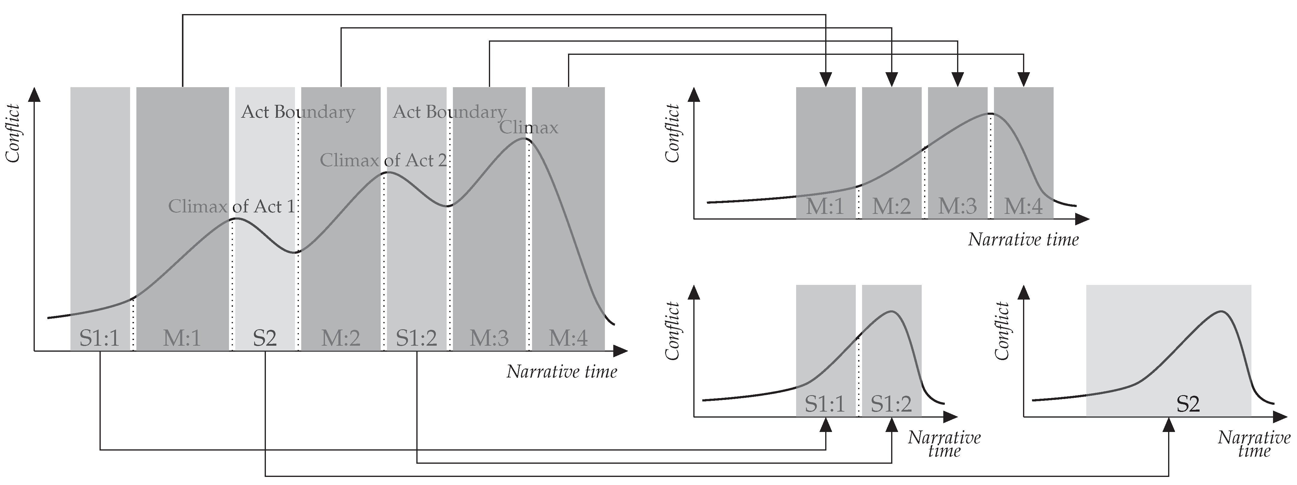Character networks exhibited a noticeable performance in extracting fragmentary information from stories, e.g., importance of characters [2,4,15], communities among characters [2,3,6], major events [6,16], and so on. Nevertheless, features that character networks reflect are far not only from stories (i.e., a series of events that happen in the narrative world) but also from plots (i.e., a series of events that are logically connected). Since they have not considered context and story lines, this problem is inevitable. Moreover, stories consist of multiple story lines, and the story lines are complicatedly entangled, as described in Figure 1. This point creates difficulties in computationally analyzing stories’ context.

To analyze stories’ context, a few studies [10,11,18] have attempted to reveal plot structures of narrative works. They concentrated on discriminating story lines in a story. Although story lines in a story describe events in the same narrative world, they also have independent narrative arcs, as illustrated in Figure 1. Therefore, classifying events into story lines, which are sets of more logically connected events, is a starting point for analyzing plot structures and understanding stories’ context.

Some story lines present events around protagonists, and others deal with side branches of a story. If a story line is more focused on events related to protagonists and main conflicts, we call it ‘main plot.’ The other story lines are called ‘subplots.’ The ’plot structure’ indicates the way in which a story is interwoven with multiple subplots. Each main plot and subplot is split into multiple fragments, and authors/directors present the fragments alternatively.

A fundamental principle for composing a plot structure is that events in a story must be located to escalate conflicts around its protagonist. Therefore, models for typical plot structures (e.g., Freytag’s pyramid [19] and arch plot [17]) commonly say that conflicts in a story should be intensified until the climax and then resolved. In most of the stories, a climax is placed much closer to a denouement than an exposition to maintain users’ interests until the end [17]. Nevertheless, if conflicts are gradually escalated until the climax, users will be exhausted. Thus, in practice, authors/directors control conflicts in stories by interweaving multiple story lines, as displayed in Figure 1.

The existing studies [10,11,18] attempted to distinguish main plots and subplots based on the changes in the social relationships of characters. This approach is based on a notion that each main plot and subplot has its own protagonists and main characters [17]. Although this notion is a clear and obvious fact in narratology studies, we cannot assure the accuracy of the methods based on this notion. To classify scenes into main plots and subplots, Sang and Xu [18] compared scenes based on the occurrence frequency of characters, and Lee and Jung [10] compared structures of character networks in each scene (in narratology studies [14,17], a scene is defined as a period without changes in backgrounds. In addition, a scene describes a concluded event that happened in a spatio-temporal background. Therefore, we use a scene as the smallest unit of a story to distinguish events in the story.). However, both of the methods could not exhibit a reliable accuracy [11]. As Bost et al. [16] discussed, social relationships between characters change according to stories’ development, and these changes are more dramatic around major events.

To solve this problem, we focus on that each main plot and subplot has its own plot structure [17]. Thus, they also have their own conflicts, climaxes, protagonists, and so on. According to Robert McKee [17], conflicts and events are also designed to jeopardize the everyday lives of protagonists and cause changes in characters’ personalities in a consistent direction. Our problem (i.e., changes in social relationships) is only the result of the changes in personalities. These points indicate that characters will show gradual changes in each main plot and subplot. Therefore, if we can discover features that reflect the characters’ personalities, we also can classify scenes by making the features show gradual increments or decrements. The fundamental assumption of this study can be clarified as follows:

Assumption 1

(Dynamic Changes in Personalities of Characters). Conflicts in a story are designed to motivate so that its protagonist or main character changes himself/herself. In most of the stories, this change is uni-directional. Thus, if a character’s personality is not static, this change progresses from a state (A) to another state (B) according to narrative time from an inciting incident to the climax of the story. At the climax, the change is concluded as A, B, or somewhere else between A and B.

Assumption 2

(Independence of Subplots). A story is mostly interwoven with a main plot and multiple subplots. Although the subplots function to support the main plot, they are also independent story lines with their own conflicts, protagonists, and main characters. Therefore, characters’ personalities exhibit uni-directional tendencies in a single subplot.

Nevertheless, in real narrative works, main plots and subplots are complicatedly entangled, and transitions between them frequently happen. Thus, if we analyze characters’ changes according to scenes’ order, the changes might seem irregular and noisy. We use this problem to solve the problem itself. If a plot structure is impeccably decomposed into main plots and subplots, characters’ personalities will show gradual changes in each of them.

Based on this notion, we propose methods for computationally decomposing the plot structures of stories. First, we suggest features for capturing changes in characters’ personalities. By drawing trend curves of the features, we can reveal ways how the characters change. Then, we extract the primary story line by knocking out noisy scenes, which are far from the trend curves. By iteratively conducting this process, we discover main plots and subplots, one-by-one. We have validated these assumptions and evaluated the proposed methods based on real movies.

This study focuses on enabling an in-depth analysis of narrative multimedia by revealing plot structures. However, plot structure decomposition can also improve practical applications of computational narrative analysis. For example, the existing methods for story-based summarization [12,20,21,22,23] concentrated on extracting more important scenes than others. They employed various criteria to measure importance, such as whether protagonists appear in the scenes. However, since they do not consider causalities between scenes, they cannot deal with the abstractive summarization. The proposed methods can be applied to resolving this issue because a story line is a set of scenes that have causal relationships. This point is similar in other applications: Story-based recommendation [6] or indexing [13,24]. We will present more details in Section 5 with further research directions.

The remainder of this paper is organized as follows. Section 2 presents the backgrounds of this study and the existing studies for analyzing plots. In Section 3, we propose the features for fictional characters’ personalities and the methods for decomposing plot structures by analyzing changes in the personalities. In Section 4, we evaluate the proposed methods and validate our assumptions. Section 5 presents concluding remarks and further research directions.

2. Preliminaries and Literature Review

Despite studies for the character network and applications based on this model during recent years [25], it is still an unfamiliar research area for most of the scholars in computer science. Therefore, we present an overview of (i) concepts and definitions related to the character network model and (ii) the existing approaches for analyzing plot structures by using the character network.

2.1. Character Networks and Plot Structures

According to John Truby [14], stories are developed by interactions between protagonists and their surrounding characters. From this intuition, various studies [2,3,4,5,6,9,26] have attempted to model and analyze stories based on the social networks of characters that have appeared in the stories. Nodes of the social networks are characters, and edges represent interactions between the characters. We call these social networks of characters ‘character networks’.

Since narrative works and stories are time-sequential, the existing studies [6,9,27] have defined the character network as a dynamic social network. They attempted to analyze stories’ development based on how character networks dynamically evolve. The dynamic character network is made by segmenting narrative works into regular units (e.g., scenes) and composing character networks on each unit.

We can choose an appropriate unit by considering (i) media and formats of narrative works and (ii) tasks that we deal with (e.g., recommendation, indexing, and summarization). For example, according to narratology studies [17,28], a movie consists of 3 to 4 acts, an act consists of 3 to 6 sequences, and a sequence consists of 2 to 5 scenes. This study employs the scene as the regular unit since there have not been methods for automatically discovering acts or sequences from visual narrative works with enough accuracy, to the extent of our knowledge [29,30,31,32,33,34,35]. The character network has been defined as follows:

Definition 1

(Character Network [9,10]). Suppose that N is the number of characters that appeared in the α-th narrative work, ${\mathbb{C}}_{\alpha }$. When $N\left({\mathbb{C}}_{\alpha }\right)$ indicates a character network of ${\mathbb{C}}_{\alpha }$, and $\mathbb{R}$ refers to the real number, $N\left({\mathbb{C}}_{\alpha }\right)$ can be defined as a matrix $\in {\mathbb{R}}^{N\times N}$. Each component of $N\left({\mathbb{C}}_{\alpha }\right)$ indicates a degree of proximity between two characters.

By segmenting ${\mathbb{C}}_{\alpha }$, we transform $N\left({\mathbb{C}}_{\alpha }\right)$ into a dynamic social network. When ${\mathbb{C}}_{\alpha }$ includes L scenes, $s_{\alpha ,l}$ is the l-th scene of ${\mathbb{C}}_{\alpha }$, and $N\left(s_{\alpha ,l}\right)$ indicates a character network only within $s_{\alpha ,l}$, a relationship between $N\left({\mathbb{C}}_{\alpha }\right)$ and $N\left(s_{\alpha ,l}\right)$ can be formulated as:

$$\begin{array}{c}\hfill N\left({\mathbb{C}}_{\alpha }\right)=\sum _{l=1}^{L}N\left(s_{\alpha ,l}\right)=\left[\begin{array}{ccc}{a}_{1,1}& \cdots & a_{1,N}\\ ⋮& \ddots & ⋮\\ a_{N,1}& \cdots & a_{N,N}\end{array}\right],{\mathbb{C}}_{\alpha }=〈s_{\alpha ,1},\cdots ,s_{\alpha ,l},\cdots ,s_{\alpha ,L}〉,\end{array}$$

(1)

where $a_{i,j}$ indicates proximity of $c_i$ for $c_j$ when $c_i$ is the i-th character that appeared in ${\mathbb{C}}_{\alpha }$.

For composing character networks and measuring proximity, various methods and models have been proposed [2,3,4,5,6,9,26,36,37,38,39]. In this study, we use lingual character networks proposed by Lee and Jung [9]. This model estimates the proximity, based on dialogue frequency between characters, similar to the conventional models [3,15,24,40]. However, it can measure the proximity more accurately by considering that a scene can contain multiple conversations. Thus, while the existing dialogue-based character networks suppose that all characters in a scene are listeners of all dialogues spoken in the scene, we limit listeners into participants of each conversation. Lee and Jung [9] also compared various character network models. This comparison lets us know that participating in conversations is a significant feature by itself. Thus, we consider the number of dialogues and conversations that each character is involved in. In addition, not only frequency of dialogues but also lengths of dialogues are meaningful for analyzing story flow, especially in major event detection [41]. Thus, we also annotate the number of words in dialogues on character networks. This can be formulated as:

$$\begin{array}{c}\hfill a_{i,j}=〈n_{i,j},w_{i,j},b_{i,j},c_{i,j}〉,\end{array}$$

(2)

where $n_{i,j}$ indicates the total number of dialogues from $c_i$ to $c_j$, $w_{i,j}$ refers to the number of words in the dialogues, $b_{i,j}$ denotes the number of dialogues exchanged between $c_i$ and $c_j$, and $c_{i,j}$ indicates the number of conversations that $c_i$ and $c_j$ participate in together. In addition, for an orthogonal element $a_{i,i}$, $n_{i,i}$ indicates the number of dialogues spoken by $c_i$, $w_{i,i}$ denotes the number of words in the spoken dialogues, $b_{i,i}$ refers to the number of dialogues spoken or listened by $c_i$, and $c_{i,i}$ denotes the number of conversations that $c_i$ participate in. Figure 2 presents a character network extracted from a movie, ‘Good Will Hunting’ (1997).

In narratology, a story is defined as a sequence of events, and a plot is defined as a sequence of logically connected events. Obviously, all the events in a story are related to each other somehow. However, some events are connected more closely than others (e.g., causal relationships). And those events compose a story line. Among the story lines, ‘main plot’ is a story line that is most tightly connected to protagonists and the story’s major events.

However, defining granularity and boundaries of events is ambiguous since an event consists of smaller events, and the event can also be a part of a bigger event. Thus, we suppose that a scene corresponds to an event. Since a scene is defined as a period without changes in spatio-temporal backgrounds, a scene usually describes a concluded event.

Accordingly, in this study, main plots and subplots are defined as sequences of scenes. In addition, within a main plot or a subplot, scenes should be more connected with each other than with scenes outside. The subplot can be defined as follows:

Definition 2

(Subplot [10]). When ${\mathcal{P}}_n^s$ is the n-th subplot in ${\mathbb{C}}_{\alpha }$ and includes $s_{\alpha ,i}$ and $s_{\alpha ,j}$, $s_{\alpha ,i}$ and $s_{\alpha ,j}$ have a higher relevancy to each other than other scenes in ${\mathbb{C}}_{\alpha }$. This can be formulated as:

$$\begin{array}{c}\hfill {\mathcal{P}}_n^s = \left\{s_{\alpha ,i}|s_{\alpha ,j}=\underset{\forall s_{\alpha ,k}}{argmax}\mathcal{R}\left(s_{\alpha ,i},s_{\alpha ,k}\right),s_{\alpha ,j}\in {\mathcal{P}}_n^s\right\},\end{array}$$

(3)

where $\mathcal{R}\left(s_{\alpha ,i},s_{\alpha ,j}\right)$ indicates relevancy between events described in $s_{\alpha ,i}$ and $s_{\alpha ,j}$.

Authors/directors do not present these main plots and subplots separately. They compose an entire plot structure by interweaving the main plots and subplots. Therefore, decomposing a plot structure into the story lines is significant for understanding what kinds of stories are delivered by narrative multimedia.

2.2. Plot Analysis Based on Character Networks

This section introduces a few studies that have attempted to analyze plots in narrative multimedia based on the character network. Although various studies claimed their contributions to be analyzing or extracting plots, they used the term ‘plots’ to mean context or flow of stories. Therefore, most of the existing studies have not considered that a plot is interwoven with plural main plots and subplots. However, without understanding how main plots and subplots are entangled, we cannot distinguish which scenes are main plots. In addition, to find the meanings and functions of each scene, revealing plot structures is necessary.

Micha Elsner [42,43] attempted to compare plot structures in novels. The author has proposed a method for measuring the similarity of plot structures based on the similarity of characters. The character similarity was estimated by using three features: (i) Social relationships between characters, (ii) emotional words, and (iii) descriptive words that are used to describe characters. The author has also proposed a kernel function for measuring character similarity based on time-sequential changes in the three features. To extend character similarity to plot structure similarity, the author calculated similarity between all characters that appeared in two novels. The plot structure similarity between the two novels was estimated by a summation of all the similarities between characters from each novel. In the studies of Elsner [42,43], the plot structure indicates dynamic changes in characters regarding both (i) changes in each character and (ii) compositions of the characters. Finally, the author attempted to represent plot structures by using time-sequential fluctuations of the three features. Changes in characters might partially reflect connectivity between events since the events cause and trigger the changes. Nevertheless, this approach oversimplifies the plot structure. Since a plot structure is interwoven with multiple story lines, we have to consider that characters will show different directions (or amount) of changes in each story line. The methods of Elsner [42,43] will be applicable after decomposing plot structures into individual story lines.

Graham Alexander Sack [44] proposed a method for simulating plot structures. This method uses a similar approach to the study of Elsner [43] but is much simpler. The author attempted to expose transitions between story lines by using changes in the occurrence frequency of names of each character. This approach assumes that the frequency of names reflects how much a story is focused on each character (called ‘narrative attention’). Sack [44] also proposed a method for simulating the narrative attention and interactions between characters. However, the purpose of this simulation is not to decompose plot structures into story lines but to combine story lines into an optimal plot structure. In another study, Sack [45] also proposed a method for simulating changes in character networks to generate stories from character networks.

Reagan et al. [46] have discovered typical plots of novels by clustering the novels according to time-sequential changes in sentiments. Similar to the study of Dara Marks [47], they measured the sentiments of words in novels and modeled changes in the sentiments time-sequentially. They named this model ‘emotional arc.’ Although they found six typical plots by clustering the emotional arcs, this approach is too superficial to analyze plots semantically. Since these three approaches [43,44,46] focused on textual narrative works (e.g., novels), it is difficult to expand them to various kinds of narrative multimedia. However, they commonly exhibited a necessity of a time-sequential analysis of plots.

A few studies have proposed methods for decomposing plot structures into story lines. However, as we discussed, most of these studies only relied on occurrences of characters or relationships between characters. Liang et al. [32] and Sang and Xu [18] have proposed methods for segmenting movies into narrative units in multiple layers (shots ∈ scenes ∈ sub-stories). They aimed to compose sub-stories as a set of scenes that contains scenes describing related events. Thus, the ‘sub-story’ is conceptually the same as story lines in this study (main plots or subplots). From scenes to story lines, they applied the hidden Markov model, which has occurrences of characters in each scene as observations and story lines containing the scene as hidden states. This approach was applied to discovering scenes likewise. Nevertheless, scenes in a story line do not always have identical occurrence distributions of characters. Subsequently, Sang and Xu [18] summarized movies by applying a top-down selection for entities on the three-layered structure according to the significance of the entities. They measured the significance with three criteria: (i) The number of characters that appeared in an entity, (ii) the number of main characters among the appeared characters, and (iii) the number of dialogues spoken by the main characters.

Xavier Bost [20] applied the time-sequential characteristics of stories on identifying story lines in TV series. They assumed that social relationships between characters have consistent tendencies in a story line. From this assumption, they proposed two measurements for the persistence and anticipation of social relationships. The two measurements were estimated based on (i) out-degrees of main characters and (ii) proximity between the main characters. They detected transitions between story lines by using changes in the measurements. However, in narrative multimedia, fragments of story lines are located alternatively. Thus, to decompose plot structures, we also need to reassemble story lines by combining the fragments.

Lee and Jung [10] decomposed plot structures by using structural changes in character networks. They applied interactions on each scene to measure relevancy between events described in the scenes. By embedding character networks on each scene (e.g., $N\left(s_{\alpha ,l}\right)$), they calculated ‘narrative relevancy’ between $s_{\alpha ,i}$ and $s_{\alpha ,j}$ based on similarity between vector representations of $N\left(s_{\alpha ,i}\right)$ and $N\left(s_{\alpha ,j}\right)$. Then, story lines were obtained by clustering scenes according to narrative relevancy. In addition, to discover main plots and major events, they measured the significance of scenes. Similar to the study of Lee and Jung [6], they measured the ‘narrative significance’ of each scene based on how much the scene changes relationships between characters. The narrative significance of $N\left(s_{\alpha ,l}\right)$ was measured by comparing ${\sum }_{i=1}^{l}N\left(s_{\alpha ,i}\right)$ and ${\sum }_{i=1}^{l-1}N\left(s_{\alpha ,i}\right)$ by embedding them. Although Lee and Jung [10] presented only theoretical models, O-Joun Lee [11] exhibited the efficacy of this approach with real movies.

However, as Bost et al. [16] discussed, there studies commonly ignore that relationships between characters significantly change around major events (especially climaxes). Furthermore, the compositions of characters in each story line are not always consistent. For example, in the movie ‘The Godfather’ (1972), even its protagonist, ‘Michael Corleone’, did not appear in many scenes that are in its main plot. To solve this issue, we propose methods for modeling gradual changes in character personalities and applying the changes for decomposing plot structures.

3. Plot Structure Decomposition-Based Personalities of Characters

Plot structures of narrative works are interwoven with multiple story lines (subplots). This study aims to decompose plot structures into subplots and discover the primary subplot (main plot). We conduct the decomposition by analyzing dynamic changes in character personalities. This approach is based on two assumptions. The previous studies [10,11,18] attempted to discriminate subplots based on the consistency of social relationships between characters. Nevertheless, these studies overlooked that (i) relationships of characters significantly change around major events (e.g., inciting incidents or climaxes), and (ii) not all the main characters are involved in all the events in a subplot. We solve this problem with an assumption that the protagonists and main characters of a subplot will be consistently and relatively more important than other characters in the subplot.

Second, characters change according to the stories’ flows, but they mostly show gradual changes until the end or return to the original states after climaxes [17,28]. Furthermore, the changes usually happen to the protagonists and main characters. Roughly speaking, a character can have various roles in each subplot, and, in a subplot, their personality will be static or will gradually change. Thereby, if we have a measurement for quantifying the personality, the measurement for a character in a subplot will be linear or convex for the narrative time.

Therefore, we first attempt to discover features that can reflect personality changes. We assume that changes in social relationships of characters are the results of changes in their personalities. Based on the features, we propose methods for (i) detecting transitions between subplots and (ii) clustering scenes into subplots.

3.1. Revealing Personality Changes of Characters

The existing studies for discovering connectivity between events (scenes) have assumed that correlated scenes present the similar social relationships of characters [10,11,18]. However, as discussed in the previous sections, social relationships change even in a story line, particularly around major events [16]. In addition, not all characters in a story line consistently appear in all of the scenes of the story line.

To solve this problem, we attempt to utilize the changes themselves. From Assumptions 1 and 2, we suppose that changes in social relationships are results of changes in personalities of characters, and the changes are uni-directional (e.g., passiveness to activeness) at least in each story line. Therefore, in this section, we propose three features for detecting the personality changes of characters.

First, we define a feature that can be relatively robust to personality changes. According to McKee [17,28], each main plot and subplot has its own protagonist and main characters, and these roles are static. The existing studies [2,4,15] defined ‘importance of characters’ as node centrality of the characters in their social network, in order to classify characters into the roles (e.g., protagonist, main, minor, and extra characters). Thus, in other words, although a protagonist and a main character established a new relationship after a climax, the protagonist will still have higher centrality than the main character. In addition, regardless of absences of a few characters in a few scenes, the relative importance of each character is consistent; when $c_i$, $c_j$, and $c_k$ are the protagonist, main, and minor characters of a story line, respectively, $c_j$ will have higher centrality than $c_k$ in most scenes in the story line whether $c_i$ appear with them or not. We measure the importance by using how many interactions (e.g., dialogues and conversations) each character is involved in (i.e., degree centrality).

In the movie ‘The Godfather’ (1972), the protagonist ‘Michael Corleone’ gradually changes from a passive stance to an active stance for his family business. In the character networks of this movie, the out-degree of ‘Michael Corleone’ becomes larger according to the flow of the stories, compared to its in-degree. However, when we simply see interaction frequency, ‘Michael Corleone’ has been consistently involved in most of the dialogues and conversations within the scenes that he appears in.

To measure importance, we consider the interaction frequency in terms of two aspects: The number of dialogues ($b_{i,i}$ in Equation (2)) and conversations ($c_{i,i}$ in Equation (2)) that each character is involved in. $b_{i,i}$ provides us how salient $c_i$ was in a scene. Although $c_i$ was mostly a listener, authors/directors might not place them without any reason. We have also supposed that a scene describes an event due to the difficulties in discriminating and segmenting events. However, events consist of smaller events, and the events compose bigger events. $c_{i,i}$ lets us know whether $c_i$ participates in all minor events happened in a scene.

For assessing consistency of characters’ importance, we have to normalize the importance. The normalized importance is called ‘relative importance’ and is defined as follows:

Definition 3

(Relative Importance). Relative importance of $c_i$ during $s_{\alpha ,l}$ ($I(c_i,s_{\alpha ,l})$) indicates how important $c_i$ was on $s_{\alpha ,l}$ compared with other characters that appeared in $s_{\alpha ,l}$. For a scene $s_{\alpha ,l}$, when $b_{i,i}$ and $c_{i,i}$ indicate the number of dialogues and conversations that $c_i$ participated in during $s_{\alpha ,l}$, respectively, $I(c_i,s_{\alpha ,l})$ is estimated by a linear combination of normalized $b_{i,i}$ and $c_{i,i}$. We can also compose a vector for representing the importance of all the characters that appeared in ${\mathbb{C}}_{\alpha }$. This can be formulated as:

$$\begin{array}{ccc}& & \overrightarrow{I}\left(s_{\alpha ,l}\right)=〈I(c_1,s_{\alpha ,l}),\cdots ,I(c_i,s_{\alpha ,l}),\cdots ,I(c_N,s_{\alpha ,l})〉,\hfill \end{array}$$

(4)

$$\begin{array}{ccc}& & I(c_i,s_{\alpha ,l})=(1-{\mathcal{W}}_C)\times \frac{b_{i,i}}{{max}_{\forall c_j}{b}_{j,j}}+{\mathcal{W}}_C\times \frac{c_{i,i}}{{max}_{\forall c_j}{c}_{j,j}},\hfill \end{array}$$

(5)

where ${\mathcal{W}}_C$ denotes a weighting factor for conversations. In addition, when $b_{i,i}=0$, $I(c_i,s_{\alpha ,l})=Ø$.

Thus, $I(c_i,s_{\alpha ,l})\in [0,1]$ has a higher value, as characters have a relatively larger portion for events described in $s_{\alpha ,l}$. $I(c_i,s_{\alpha ,l})$ includes importance based on two features: Dialogue and conversations. At this moment, we cannot assure which feature is more robust to changes in the social relationships of characters. Thus, we will conduct a hyper-parameter search to find out the optimal ${\mathcal{W}}_C$ based on experiments with real movies.

The relative importance and features used in the existing studies [6,10,11,18,48] have commonly relied on only changes in social relationships between characters. However, as discussed in various studies [16,17], social relationships significantly change around major events. Moreover, strictly speaking, the changes in relationships are a partial reflection of changes in the inner sides of the characters [17,28].

Furthermore, McKee [17] said that characters in stories are designed and allocated to cause events and escalate conflicts around their protagonists. Thus, the events are drawn to raise inner or outer conflicts around protagonists, and changes caused by the conflicts are concentrated mostly on protagonists and main characters rather than minor ones, which are far from protagonists.

However, it is challenging to quantify changes in the personalities of characters. Although various methods have been proposed to recognize the meanings of facial and vocal expressions of actors/actresses or emotional words in dialogues, these methods have still focused on meanings of a single expression rather than pragmatic meanings [49,50]. Dialogues in visual narrative works are closer to everyday language than in textual narrative works (e.g., novels) [17,28]. Thus, it is difficult to simply use emotional words in narrative works for detecting personality changes or analyzing plot structures, as case studies on novels [42,43,44,46].

This study applies simple statistical features, which are already validated by the existing studies in the computational narrative analysis. We measure inner changes of characters by using (i) average lengths of dialogues [28,41,51] and (ii) ratios of out-degree for in-degree [47]. Although these features are simple and intuitive, they have exhibited reliable performance for analyzing flows of stories in the existing studies.

The average length of dialogues is based on ‘two clock theory’ in psychology studies [41]. However, its concept is quite intuitive and obvious. Let suppose that there is an action movie, and dialogue in the movie is mostly exclamations. If the protagonist and antagonist exchange a long piece of dialogue in a scene, the scene might be a major event (e.g., revealing secrets, resolving conflicts, and so on). Zvi Lotker [41] and Liu et al. [51] have attempted to detect major events in stories based on the average lengths of all dialogues in each scene. However, they conducted experiments with narrative works that have relatively simple plot structures with few subplots (e.g., plays of Shakespeare and TV animation series). Thus, in this study, we analyze both the average dialogue lengths (i) for all characters and (ii) for each character. This feature can be defined, as follows:

Definition 4

(Average Lengths of Dialogue). The average length of dialogue spoken by $c_i$ during $s_{\alpha ,l}$ ($L(c_i,s_{\alpha ,l})$) indicates how long $s_{\alpha ,l}$ is in feeling of $c_i$. For a scene $s_{\alpha ,l}$, when $n_{i,i}$ and $w_{i,i}$ indicate the number of dialogues spoken by $c_i$ and the number of words in the dialogues, respectively, $I(c_i,s_{\alpha ,l})$ is estimated by a ratio of $w_{i,i}$ for $n_{i,i}$. In addition, by averaging lengths of all the dialogues in $s_{\alpha ,l}$ ($L\left(s_{\alpha ,l}\right)$), we can represent changes in tempos of storytelling [11,41]. This can be formulated as:

$$\begin{array}{ccc}& & \overrightarrow{L}\left(s_{\alpha ,l}\right)=〈L(c_1,s_{\alpha ,l}),\cdots ,L(c_i,s_{\alpha ,l}),\cdots ,L(c_N,s_{\alpha ,l})〉,\hfill \end{array}$$

(6)

$$\begin{array}{ccc}& & L\left(s_{\alpha ,l}\right)=\underset{\forall c_i,a_{i,i}\ne Ø}{mean}L(c_i,s_{\alpha ,l}),L(c_i,s_{\alpha ,l})=\frac{w_{i,i}}{n_{i,i}}.\hfill \end{array}$$

(7)

In addition, when $n_{i,i}=0$, $L(c_i,s_{\alpha ,l})=Ø$.

We anticipate that the average length of dialogues gets larger, when inner conflicts of a character become intensified. Furthermore, as external conflicts escalate, the average length might be smaller.

The ratio of out-degree for in-degree is widely-used in the SNA (Social Network Analysis) area for estimating the ‘activeness’ of users or entities. Marks [47] has discussed that the activeness of main characters gradually fluctuates with changes in the personalities of the characters based on various real movies. If a character is active, they will speak dialogues more frequently than listen to the dialogues of other characters, and the character’s out-degree will be higher than their in-degree. As we discussed, ‘Michael Corleone’ in ‘The Godfather’ (1972) shows gradual changes in his stance for the family business (from passive to active). These changes are exposed when he starts participating in conversations within his family as a speaker rather than a listener. As a contrary case, ‘Clark Kent’ in ‘Superman’ (1978) is a static character and always leads most of the events. Thus, ‘Clark Kent’ has a higher out-degree than in-degree consistently. For the normalization, we measure the activeness as a ratio of the number of spoken dialogues for the number of dialogues both spoken and listened to. This feature can be defined, as follows:

Definition 5

(Ratios of Out-degrees for In-degrees). The ratio of out-degree of $c_i$ for its in-degree on $s_{\alpha ,l}$ ($A(c_i,s_{\alpha ,l})$) indicates how active $c_i$’s stance is during $s_{\alpha ,l}$. For a scene $s_{\alpha ,l}$, when $n_{i,i}$ and $b_{i,i}$ indicate the number of dialogues spoken by $c_i$ and of all the dialogues spoken and listened by $c_i$, respectively, $A(c_i,s_{\alpha ,l})$ is estimated by a ratio of $n_{i,i}$ for $b_{i,i}$. In addition, using the entropy of $A(c_i,s_{\alpha ,l})$ for all characters in $s_{\alpha ,l}$, we can represent whether interactions in $s_{\alpha ,l}$ is led by few characters or all the characters have a right to speak. This can be formulated as:

$$\begin{array}{ccc}& & \overrightarrow{A}\left(s_{\alpha ,l}\right)=〈A(c_1,s_{\alpha ,l}),\cdots ,A(c_i,s_{\alpha ,l}),\cdots ,A(c_N,s_{\alpha ,l})〉,\hfill \end{array}$$

(8)

$$\begin{array}{ccc}& & A\left(s_{\alpha ,l}\right)={\left[1+\underset{\forall c_i,a_{i,i}\ne Ø}{mean}-logA(c_i,s_{\alpha ,l})\right]}^{-1},A(c_i,s_{\alpha ,l})=\frac{n_{i,i}}{b_{i,i}},\hfill \end{array}$$

(9)

In addition, when $b_{i,i}=0$, $A(c_i,s_{\alpha ,l})=Ø$.

Conclusively, a feature vector for personality changes of characters on a scene $s_{\alpha ,l}$ (${\mathcal{F}}_{\alpha ,l}$) can be formulated as:

$$\begin{array}{c}\hfill {\mathcal{F}}_{\alpha ,l}=\overrightarrow{I}\left(s_{\alpha ,l}\right)\oplus \overrightarrow{L}\left(s_{\alpha ,l}\right)\oplus 〈L\left(s_{\alpha ,l}\right)〉\oplus \overrightarrow{A}\left(s_{\alpha ,l}\right)\oplus 〈A\left(s_{\alpha ,l}\right)〉,\end{array}$$

(10)

where ⊕ indicates the concatenation operation between vectors. For the proposed features, we assume that relative importance (Definition 3) will be consistent in each main plot and subplot. The other two features (Definitions 4 and 5) will show gradual and uni-directional changes in each story line. Figure 3 presents time-sequential changes in the proposed features within a real movie, ‘Good Will Hunting’ (1997). In the following sections, we propose methods for discovering main plots and subplots based on the proposed features.

3.2. Plot Structure Decomposition

To discover the main plots and subplots, we concentrate on a point that the personalities of protagonists or main characters change according to stories’ development, and the changes have consistent directions, at least in each story line. Obviously, in some stories, the personalities of the main characters do not change (e.g., the ‘Superman’ series) or come back to the beginning. Nevertheless, most of the stories have one common point: The inner changes are caused by inciting incidents and gradually progress until the denouement. Thereby, when we define time-serial functions based on the proposed features and narrative time, the functions’ shapes will be linear or convex in a story line.

First, we define time-serial functions for each character for the three features: $I_{c_i}\left(s_{\alpha ,l}\right)$, $L_{c_i}\left(s_{\alpha ,l}\right)$, and $A_{c_i}\left(s_{\alpha ,l}\right)$. If we reduce the domains of these functions from an entire narrative work (${\mathbb{C}}_{\alpha }=〈s_{\alpha ,1},\cdots ,s_{\alpha ,L}〉$) to a main plot or subplot in ${\mathbb{C}}_{\alpha }$ (${\mathcal{P}}^M$ or ${\mathcal{P}}_n^s$), the three functions will be linear or convex for narrative time (l). Thus, we subsequently conduct the linear and quadratic regression for the functions. By searching for an optimal regression model, we can trace the personality changes of each character in the most significant story line, which is latent in the search space. For example, if we conduct regression for an entire story, we will obtain the directions of changes in its main plot. When $F_{\alpha ,l}\left(i\right)$ indicates the i-th component of the feature vector (in Equation (10)), this can be formulated as:

$$\begin{array}{ccc}& & {\widehat{F}}_{\alpha ,l}\left(i\right)=\left\{\begin{array}{cc}{\theta }_0\times l+b_0,\hfill & \mathrm{for}\mathrm{linear}\mathrm{regression},\hfill \\ {\theta }_2\times l^2+{\theta }_1\times l+b_1,\hfill & \mathrm{for}\mathrm{quadratic}\mathrm{regression}.\hfill \end{array}\right.,\hfill \end{array}$$

(11)

$$\begin{array}{ccc}& & \mathcal{L}\left(F\left(i\right)\right)=\sum _{\begin{array}{c}{s}_{\alpha ,l}\in {\mathbb{S}}_{\alpha },\\ F_{\alpha ,l}\left(i\right)\ne Ø\end{array}}{∥{\widehat{F}}_{\alpha ,l}\left(i\right)-F_{\alpha ,l}\left(i\right)∥}_2,\hfill \end{array}$$

(12)

where ${\mathbb{S}}_{\alpha }$ indicates a current search space, ${\widehat{F}}_{\alpha ,l}\left(i\right)$ denotes a predicted value of the i-th component on $s_{\alpha ,l}$, and $\mathcal{L}\left(F\right(i\left)\right)$ refers to a loss of the regression model for the i-th components, which is measured by l-2 norm (mean square error). The regression model, which represents a tendency of the i-th components in the search space (${\mathbb{S}}_{\alpha }$), is determined by searching models and parameters that make $\mathcal{L}(·)$ minimized.

Based on the regression models, each main plot and subplot is discovered by discarding scenes with significantly higher errors than the other scenes. Simply speaking, we (i) find dominant tendencies of characters’ personality changes and (ii) filter scenes that do not accord with the tendencies. Therefore, we first compose vectors to represent errors of each scene for the features and their regression models. The vector for a scene $s_{\alpha ,l}$ (${\mathcal{L}}_{\alpha ,l}$) can be formulated as:

$$\begin{array}{c}\hfill {\mathcal{L}}_{\alpha ,l}=〈\mathcal{L}\left(F_{\alpha ,l}\left(1\right)\right),\cdots ,\mathcal{L}\left(F_{\alpha ,l}\left(i\right)\right),\cdots ,\mathcal{L}\left(F_{\alpha ,l}(3N+2)\right)〉.\end{array}$$

(13)

Each component of ${\mathcal{L}}_{\alpha ,l}$ is calculated by l-2 norm; e.g., $\mathcal{L}\left(F_{\alpha ,l}\left(i\right)\right)={\parallel {\widehat{F}}_{\alpha ,l}\left(i\right)-F_{\alpha ,l}\left(i\right)\parallel }_2$. Then, using the support vector clustering (SVC) [52], we categorize scenes into two groups that follow the tendencies and do not follow.

Based on the group, which is out of the tendencies, we redefine the search space and conduct the regression and classification again; ${\mathbb{S}}_{\alpha }\leftarrow {\mathbb{S}}_{\alpha }-{\mathcal{P}}_n$, where ${\mathcal{P}}_n$ denotes the newly discovered story line. According to changes in the number of scenes in the search space, we have to assign temporal indices for the scenes in each iteration; $l\leftarrow \widehat{l}\in [1,\left|{\mathbb{S}}_{\alpha }\right|]$. The temporal index has to preserve the original order of scenes. Thus, when two scenes ($s_{\alpha ,i}$ and $s_{\alpha ,j}$) are in ${\mathbb{S}}_{\alpha }$, $i<j\Rightarrow \widehat{i}<\widehat{j}$. By iterating these procedures, we obtain a main plot or subplot on each iteration.

In addition, the changes of personalities mostly happen in protagonists or main characters [17]. To emphasize the fluctuation in personalities, we use only main characters (including protagonists) for the regression and classification. The main characters are found by their centrality on character networks, as with the existing studies [2,4,11,15]. A set of the main characters is redefined on every iteration according to changes in the search space and the targeted story line. In addition, the character network defined in this study contains multiple weights on its edges. For measuring centrality degrees of characters, we only use the number of words spoken by each character ($w_{i,j}$ in Equation (2)).

The iterations are conducted, while scenes in the discovered story line show more distinct tendencies than all the scenes in the search space. Therefore, when ${\mathcal{P}}_n$ is a story line discovered from ${\mathbb{S}}_{\alpha }$, we conduct the regression for ${\mathcal{P}}_n$, again. Then, if a loss for ${\mathcal{P}}_n$ ($\mathcal{L}\left({\mathcal{P}}_n\right)={\sum }_{s_{\alpha ,l}\in {\mathcal{P}}_n}{∥{\mathcal{L}}_{\alpha ,l}∥}_2/\left|{\mathcal{P}}_n\right|$) is smaller than the loss for ${\mathbb{S}}_{\alpha }$ ($\mathcal{L}\left({\mathbb{S}}_{\alpha }\right)={\sum }_{s_{\alpha ,l}\in {\mathbb{S}}_{\alpha }}{∥{\mathcal{L}}_{\alpha ,l}∥}_2/\left|{\mathbb{S}}_{\alpha }\right|$), we move on to the next iteration. Otherwise, we discard ${\mathcal{P}}_n$ and finish the plot structure decomposition. For the two losses, errors for each scene (${\mathcal{L}}_{\alpha ,l}$) are composed based on different regression models, which are trained in ${\mathcal{P}}_n^s$ and ${\mathbb{S}}_{\alpha }$, respectively. Algorithm 1 describes the overall procedures of the proposed plot structure decomposition method. Furthermore, Figure 4 illustrates an empirical example of the plot structure decomposition for ‘Good Will Hunting’ (1997).

Algorithm 1 Plot Structure Decomposition

1: procedureDecomposition(${\mathbb{C}}_{\alpha }$) 2:     Initialization ${\mathbb{S}}_{\alpha }\leftarrow {\mathbb{C}}_{\alpha },{\mathcal{P}}_n\leftarrow Ø$ 3:     do 4:         ${\mathbb{S}}_{\alpha }\leftarrow {\mathbb{S}}_{\alpha }-{\mathcal{P}}_n,{\mathcal{P}}_n\leftarrow Ø,n\leftarrow n+1$ 5:         Assign temporal indices ($\widehat{l}\in [1,\left|{\mathbb{S}}_{\alpha }\right|]$) for scenes in ${\mathbb{S}}_{\alpha }$; $i<j\Rightarrow \widehat{i}<\widehat{j}$. 6:         for $i:1\to 3N+2$ do 7:            Conduct linear and quadratic regression for the i-th feature in Equation (10) 7:                   (Equation (11)). 8:            Choose adequate regression model which makes a lower MSE (Equation (12)). 9:            Calculate MSE for each scene; $\mathcal{L}\left(F_{\alpha ,l}\left(i\right)\right)\leftarrow {\parallel {\widehat{F}}_{\alpha ,l}\left(i\right)-F_{\alpha ,l}\left(i\right)\parallel }_2$. 10:         Compose error vectors for each scene (Equation (13)). 11:         Conduct the SVC for all the scenes in ${\mathbb{S}}_{\alpha }$ according to errors of the scenes. 12:         ${\mathcal{P}}_n\leftarrow \underset{\forall {\mathcal{C}}_a}{argmin}{\sum }_{s_{\alpha ,\widehat{l}}\in {\mathcal{C}}_a}\frac{{∥{\mathcal{L}}_{\alpha ,\widehat{l}}∥}_2}{\left|{\mathcal{C}}_a\right|}$ 13:         Conduct Line 5 to 10 for ${\mathcal{P}}_n$. 14:         $\mathcal{L}\left({\mathcal{P}}_n\right)\leftarrow {\sum }_{s_{\alpha ,l}\in {\mathcal{P}}_n}\frac{{∥{\mathcal{L}}_{\alpha ,\widehat{l}}∥}_2}{\left|{\mathcal{P}}_n\right|}$,   $\mathcal{L}\left({\mathbb{S}}_{\alpha }\right)\leftarrow {\sum }_{s_{\alpha ,l}\in {\mathbb{S}}_{\alpha }}\frac{{∥{\mathcal{L}}_{\alpha ,\widehat{l}}∥}_2}{\left|{\mathbb{S}}_{\alpha }\right|}$ 15:     while $\mathcal{L}\left({\mathcal{P}}_n\right)\le \mathcal{L}\left({\mathbb{S}}_{\alpha }\right)$

From the decomposition method, we can obtain story lines in order of their significance. When a story line is extracted by the proposed method, the story line describes more dominant personality changes of characters than the remaining ones, which have not been derived yet. Therefore, the most straightforward approach is designating the firstly-discovered story line as a main plot. This approach will be efficient since most of the commercial narrative works present a single protagonist and a single main plot [17,28]. However, there are also various genres and formats that employ multiple protagonists and main plots, such as omnibus movies. Therefore, the proposed methods are designed to cope with a plurality of protagonists and main plots.

Regarding our research problems, we simply defined a main plot as a story line that is more tightly connected with protagonists and main conflicts of a story than the other story lines. However, this definition is not clear enough to distinguish main plots from story lines discovered by the proposed decomposition method. For a computational definition of the main plot, we focus on that the main conflicts will cause far more significant changes in protagonists and main characters than the other minor events. A main plot is defined, as follows:

Definition 6

(Main Plot). When ${\mathcal{P}}_n^M$ is the n-th main plot in ${\mathbb{C}}_{\alpha }$, protagonists and main characters of ${\mathbb{C}}_{\alpha }$ show far more significant changes in their personalities during ${\mathcal{P}}_n^M$ than during other subplots. Thus, there will be a noticeable gap between main plots and subplots in terms of ranges of personality fluctuations. When $\mathcal{D}\left({\mathcal{P}}_n\right)$ indicates a degree of personality fluctuation in main characters during ${\mathcal{P}}_n$, we first reorder story lines in descending order according to $\mathcal{D}(·)$. The biggest gap in $\mathcal{D}(·)$ can be searched by:

$$\begin{array}{c}\hfill {\mathcal{P}}_n=\underset{\forall {\mathcal{P}}_i}{argmax}\left|\mathcal{D}\left({\mathcal{P}}_i\right)-\mathcal{D}\left({\mathcal{P}}_{i+1}\right)\right|.\end{array}$$

(14)

Subsequently, we can determine ${\mathcal{P}}_m,m\le n$ as a main plot.

The personality fluctuation is estimated by the two proposed features for character personalities: (i) The average lengths of dialogues (Definition 4) and (ii) the ratios of out-degrees for in-degrees (Definition 5). First, we measure a range of fluctuation in each main character with each feature. Then, we aggregate the ranges by summation. This can be formulated as:

$$\begin{array}{ccc}\hfill \mathcal{D}\left({\mathcal{P}}_n\right)=\sum _{c_i\in M\left({\mathbb{C}}_{\alpha }\right)}& \underset{\forall s_{\alpha ,j},s_{\alpha ,k}\in {\mathcal{P}}_n}{max}& \left|L(c_i,s_{\alpha ,j})-L(c_i,s_{\alpha ,k})\right|\hfill \\ & +\underset{\forall s_{\alpha ,j},s_{\alpha ,k}\in {\mathcal{P}}_n}{max}& \left|A(c_i,s_{\alpha ,j})-A(c_i,s_{\alpha ,k})\right|,\hfill \end{array}$$

(15)

where $M\left({\mathbb{C}}_{\alpha }\right)$ is a set of main characters composed for the entire ${\mathbb{C}}_{\alpha }$. If a story has numerous main characters whose personalities dynamically change, and these main characters are scattered over plural story lines, $\mathcal{D}(·)$ is difficult in showing significant differences between main plots and subplots. We can deal with this by applying weighting factors based on characters’ centrality (to emphasize protagonists).

Additionally, Lee [11] supposed that main plots include more scenes and have more frequent interactions between main characters than subplots. This statement seems obvious. Therefore, we also use (i) the number of scenes and (ii) the number of words spoken by main characters in each main plot and subplot as features for discriminating main plots. In the evaluation section, we will validate whether these two features improve the accuracy for distinguishing the main plots. These two features are measured and normalized as:

$$\begin{array}{c}\hfill \mathcal{L}\left({\mathcal{P}}_n\right)=\frac{\left|{\mathcal{P}}_n\right|}{\left|{\mathbb{C}}_{\alpha }\right|},\mathcal{W}\left({\mathcal{P}}_n\right)=\frac{{\displaystyle \sum _{\forall s_{\alpha ,j}\in {\mathcal{P}}_n}\sum _{\forall c_i\in M\left({\mathbb{C}}_{\alpha }\right)}{w}_{i,i}}}{{\displaystyle \sum _{\forall s_{\alpha ,k}\in {\mathbb{C}}_{\alpha }}\sum _{\forall c_i\in M\left({\mathbb{C}}_{\alpha }\right)}{w}_{i,i}}},\end{array}$$

(16)

where $w_{i,i}$ indicates the number of words in the dialogues spoken by $c_i$ on corresponding scenes (e.g., $s_{\alpha ,j}$ on numerator). We simply combine the three features ($\mathcal{D}(·)$, $\mathcal{L}(·)$, and $\mathcal{W}(·)$) by using the arithmetic mean.

A method for discriminating the main plots based on the three features is mostly similar to the method for categorizing characters according to their importance in the existing studies [2,4,11,15]. We sort all discovered story lines in descending order according to the values of the features. We calculate gaps of the feature values between story lines, which are adjacent in order. Finally, we can find out the biggest gap that separates the main plots and subplots. Figure 4 and Figure 5 show the result of the main plot discrimination for ‘Good Will Hunting’ (1997).

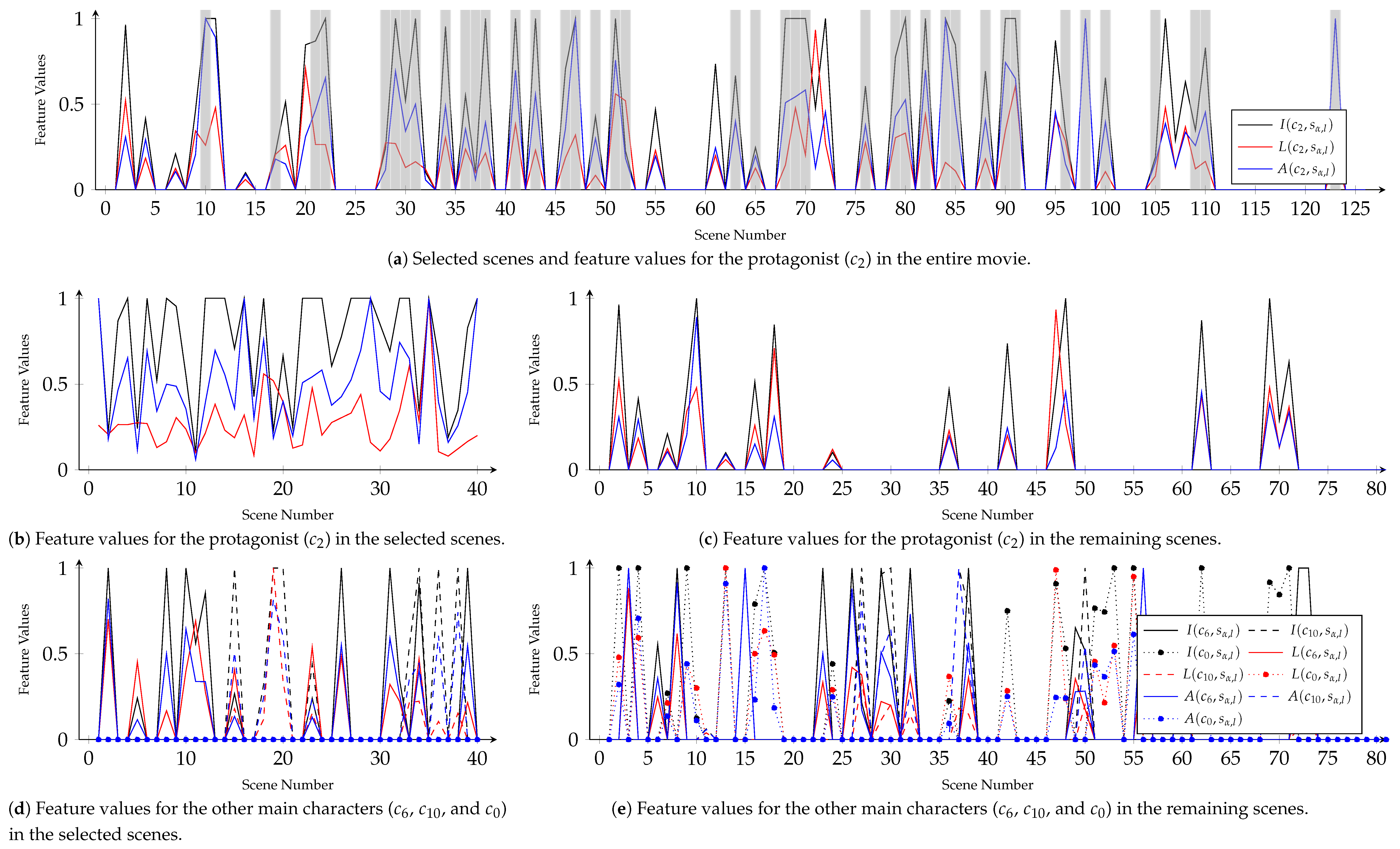
Figure 3 presents the values of three features for main characters that appeared in ‘Good Will Hunting’ (1997). Then, Figure 4 and Figure 5 present story lines discovered at the first and second iterations of the proposed decomposition method. Figure 4a shows selected scenes as a part of the first story line and values of the proposed features for ‘Will’, which is the protagonist of both the entire movie and the extracted story line. As with Figure 3, the feature values show irregular tendencies when we observe all the scenes. However, after the first iteration, the features show relatively distinguishing tendencies. Significantly, as shown in Figure 4b, the average length of dialogues spoken by ‘Will’ gradually increases. In Figure 4c, ‘Will’ appeared in a part of the remaining scenes. However, comparing Figure 4c,e, we also can see that other main characters have higher feature values in most of those scenes than ‘Will.’ Similar to Figure 3, the other main characters still show irregular tendencies in both of the selected and remaining scenes, as shown in Figure 4d,e. This point makes it difficult to say that the first story line describes relationships between ‘Will’ and other characters.We conjecture that scenes in the first story line describe events that are more connected to ‘Will’ than the others.

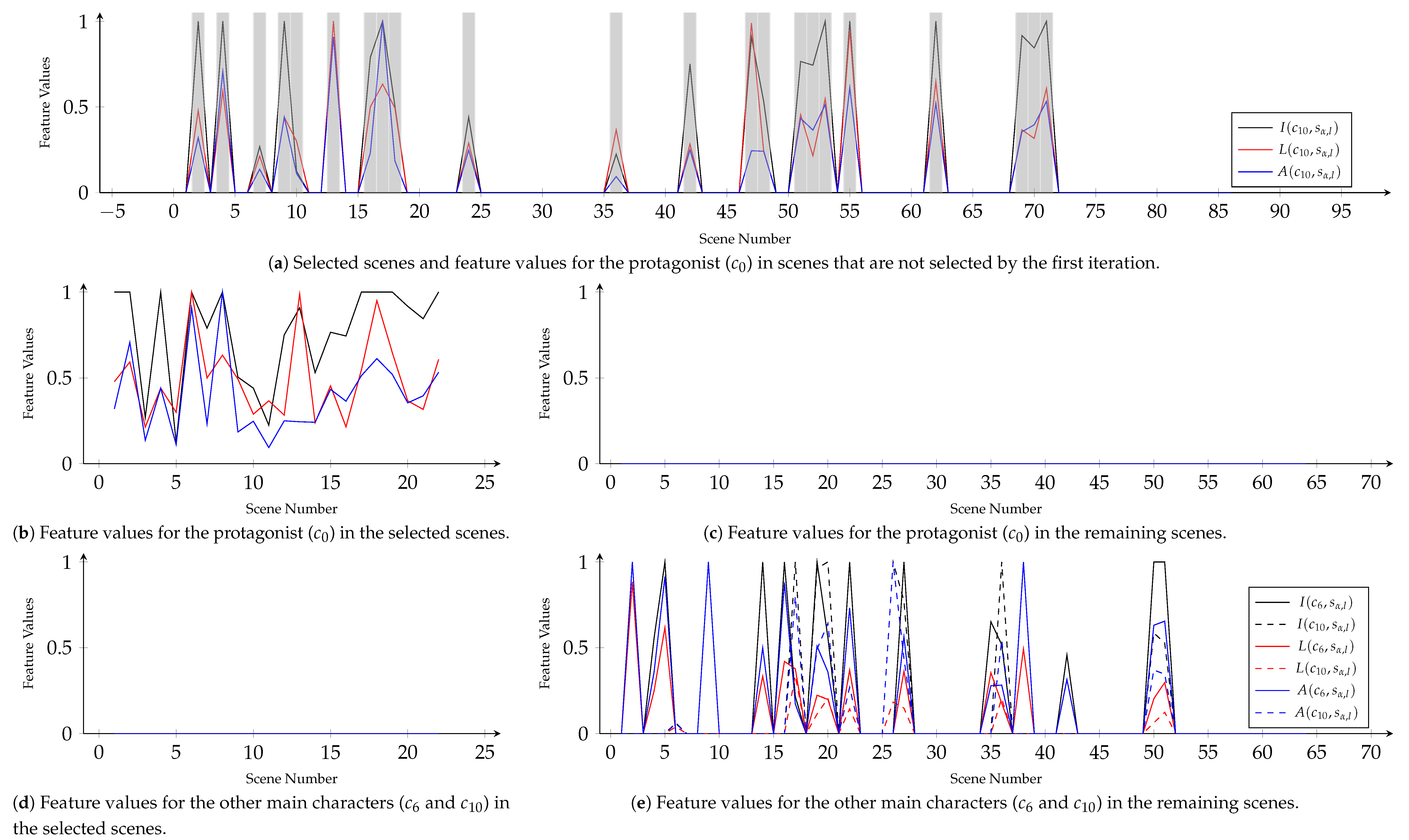
Figure 5a illustrates selected scenes as the second story line. The protagonist of this story line was ‘Chuckie’ ($c_0$). Moreover, interestingly, ‘Chuckie’ does not appear in the remaining scenes of the second iteration. The other main characters, ‘Sean’ and ‘Lambeau’ ($c_{10}$ and $c_6$), only appeared in the remaining scenes. Considering the appearance of ‘Will’, the second story line describes relationships between ‘Will’ and ‘Chuckie’, the remaining scenes seem to depict events between ‘Will’, ‘Sean’, and ‘Lambeau’ or between ‘Sean’ and ‘Lambeau.’ The remaining scenes still contain scenes in which ‘Sean’ and ‘Lambeau’ do not appear. Through the third iteration, we obtained a story line which ‘Will’ is its protagonist again. This story line describes relationships between ‘Will’ and ‘Skylar.’

Conclusively, we decomposed ‘Good Will Hunting’ (1997) into the four story lines. We asked experts in narratology to decompose this movie. Obviously, the experts’ results were different from the results of the proposed method in terms of selecting scenes in each story line. However, the main difference was that the experts divided the third story line into two parts: (i) Events between ‘Will’, ‘Sean’, and ‘Lambeau’ and (ii) conflicts between ‘Sean’ and ‘Lambeau.’ This result shows that the proposed method effectively analyzes the plot structure but should be improved. Detailed evaluation for the proposed method will be presented in the following section.

4. Evaluation

We evaluated the plot structure decomposition methods based on real movies. We also could implicitly evaluate the proposed features based on the performance of the plot structure decomposition methods. The implicit evaluation is difficult to exhibit whether the proposed features can reflect characters’ personalities and trace changes in the personalities. However, as discussed in Section 3.1, the proposed features are generalizations of the existing features for analyzing characters and events. Thus, correlations of the three features with characters’ personalities and stories’ context have been validated in the existing studies [2,4,15,41,47,51]. Moreover, it is challenging to collect reliable and large-scale data for characters’ personalities in each scene. Therefore, this study focuses on the accuracy of the proposed plot structure decomposition methods, and we evaluated features in terms of their contribution to the decomposition methods by conducting ablation tests for the features.

To assess the accuracy, we need ground truth data for the story lines of each scene. However, there have not been any benchmark dataset that include story line information at the extent of our knowledge. In addition, since classifying scenes into story lines is too abstruse for general users, we could not conduct large-scale questionnaire surveys. Therefore, we composed an expert group that consists of scholars who are faculty members of Chung-Ang University, Inha University, Kookmin University, and Sungkyunkwan University and have expertise in narratology, literature, or film studies. We compared the results of the proposed methods with ground truth annotated by the experts.

Table 1. A list of movies that have been used for evaluating the proposed methods for decomposing and analyzing plot structures.

Notation	Title	Publication Year	Genres
${\mathbb{C}}_1$	Good Will Hunting	1997	Drama, Romance
${\mathbb{C}}_2$	The Godfather	1972	Crime, Drama
${\mathbb{C}}_3$	Bruce Almighty	2003	Comedy, Drama, Fantasy
${\mathbb{C}}_4$	Wall Street	1987	Crime, Drama
${\mathbb{C}}_5$	Rain Man	1988	Drama
${\mathbb{C}}_6$	Silver Linings Playbook	2012	Comedy, Drama, Romance
${\mathbb{C}}_7$	Juno	2007	Comedy, Drama
${\mathbb{C}}_8$	American History X	1998	Drama
${\mathbb{C}}_9$	Iron Man	2008	Action, Adventure, Sci-Fi
${\mathbb{C}}_{10}$	No Country for Old Men	2007	Crime, Drama, Thriller
${\mathbb{C}}_{11}$	Up in the Air	2009	Comedy, Drama, Romance
${\mathbb{C}}_{12}$	American Hustle	2013	Crime, Drama

presents a list of the movies applied as experimental subjects.

Movies were our experimental subject since it is one of the most popular and accessible narrative multimedia. We selected the movies under the expert group’s supervision to make the dataset evenly distributed over various genres and kinds of stories. We asked the experts to suggest movies that are well-known and have multiple story lines. Since most of the suggested movies were in the drama genre, we attempted to make our experimental subjects as diverse as possible within the drama genre (e.g., crime and drama, comedy and drama, etc.). We also had to choose movies that had their scripts accessible online. Scripts and metadata of the movies were mainly acquired from IMSDb (https://www.imsdb.com/ (accessed on 11 February 2021)) and IMDb (https://www.imdb.com/ (accessed on 11 February 2021)), respectively. Then, we extracted character networks of the movies by using CharNet-Extractor, which is available through a GitHub repository (https://github.com/O-JounLee/CharNet-Extractor (accessed on 11 February 2021) and https://github.com/O-JounLee/CharNetBuilder (accessed on 11 February 2021)). The repository also includes underlying data of our running examples (Figure 2, Figure 3, Figure 4 and Figure 5). Furthermore, manual annotations of plot structures were composed for each scene in the movies. The schema of the annotation is presented in

Table 2. A list of movies that have been used for evaluating the proposed methods for decomposing and analyzing plot structures.

Item	Description	Values
Movie ID	An identifier for a movie containing this scene.	$\alpha \in [1,12]$
Scene ID	An identifier for this scene.	$l\in [1,L]$
Character List	A set of identifiers of characters that appeared in the scene.	$\{i | N{\left(s_{\alpha ,l}\right)}_{i,i}\ne 0\}$
Story Line ID	An identifier for a story line that includes this scene.	$n,s_{\alpha ,l}\in {\mathcal{P}}_n$
Flag for Main Plots	An indicator for whether this scene is included in main plots or subplots.	1 or 0
Movie Protagonist	An identifier for protagonists of this movie.	$i\in [1,N]$
Story Line Protagonist	An identifier for protagonists of this story line.	$i\in [1,N]$

.

To evaluate the effectiveness of the proposed methods for plot structure decomposition, we compared the proposed methods’ accuracy with two existing ones [10,11,18]. As a comparison group, we first used a method proposed by Sang and Xu [18]. They applied the HMM (Hidden Markov Model) on the occurrence frequency of characters to discover ‘sub-stories.’ Another existing method has been proposed by Lee and Jung [10]. They embedded social relationships between characters by learning representations of structures of character networks. Then, they clustered scenes into main plots and subplots by using vector representations.

The accuracy of each method was assessed by the precision, recall, and $F_1$ measure for each movie. For a movie, the precision and recall are calculated by ${\sum }_{\forall {\mathcal{P}}_n}|{\mathcal{P}}_n\cap {\mathcal{P}}_n^{*}|/{\sum }_{\forall {\mathcal{P}}_n}\left|{\mathcal{P}}_n^{*}\right|$ and ${\sum }_{\forall {\mathcal{P}}_n}|{\mathcal{P}}_n\cap {\mathcal{P}}_n^{*}|/{\sum }_{\forall {\mathcal{P}}_n}\left|{\mathcal{P}}_n\right|$, respectively, where ${\mathcal{P}}_n$ indicates the n-th story line annotated by the expert group, and ${\mathcal{P}}_n^{*}$ denotes ${\mathcal{P}}_n$ discovered by the decomposition methods. However, these methods are not supervised, and their results do not correspond to the manually-annotated story lines. Thereby, we have to match the manual annotations with results of the decomposition methods. ${\mathcal{P}}_n^{*}$ is determined by ${\mathcal{P}}_n^{*}={argmax}_{\forall {\mathcal{P}}_i^{*}}|{\mathcal{P}}_n\cap {\mathcal{P}}_i^{*}|$ and $|{\mathcal{P}}_n\cap {\mathcal{P}}_n^{*}|\ge \left|{\mathcal{P}}_n^{*}\right|\times 0.5$. Finally, the $F_1$ measure is calculated by the harmonic mean of the precision and recall.

To exhibit the effectiveness of the proposed features, we also evaluated each feature’s contribution to the plot structure decomposition by conducting the ablation tests. Thus, we assessed the proposed methods’ accuracy in cases where only a part of the features was used. We have proposed the three features: The relative importance (I, Definition 3), the average lengths of dialogues (L, Definition 4), and the ratios of out-degrees for in-degrees (A, Definition 5), and the assessment was conducted on all possible combinations: I, L, A, $IL$, $IA$, $LA$, and $ILA$.

Table 3. Experimental results for the accuracy of the plot structure decomposition.

Measure		I	L	A	$\mathit{IL}$	$\mathit{IA}$	$\mathit{LA}$	$\mathit{ILA}$	[18]	[10]
Precision	${\mathbb{C}}_1$	0.57	0.55	0.59	0.60	0.59	0.58	0.64	0.55	0.60
	${\mathbb{C}}_2$	0.64	0.58	0.60	0.77	0.68	0.76	0.79	0.62	0.70
	${\mathbb{C}}_3$	0.67	0.66	0.70	0.81	0.73	0.78	0.82	0.67	0.79
	${\mathbb{C}}_4$	0.65	0.64	0.62	0.78	0.69	0.78	0.78	0.74	0.74
	${\mathbb{C}}_5$	0.66	0.64	0.68	0.78	0.67	0.74	0.78	0.68	0.72
	${\mathbb{C}}_6$	0.80	0.67	0.83	0.84	0.84	0.85	0.86	0.75	0.84
	${\mathbb{C}}_7$	0.66	0.63	0.62	0.75	0.73	0.75	0.77	0.63	0.68
	${\mathbb{C}}_8$	0.63	0.53	0.59	0.69	0.70	0.70	0.64	0.59	0.64
	${\mathbb{C}}_9$	0.51	0.37	0.46	0.58	0.52	0.54	0.63	0.72	0.76
	${\mathbb{C}}_{10}$	0.63	0.60	0.62	0.74	0.65	0.73	0.71	0.63	0.67
	${\mathbb{C}}_{11}$	0.66	0.56	0.60	0.70	0.70	0.70	0.70	0.65	0.67
	${\mathbb{C}}_{12}$	0.72	0.67	0.75	0.81	0.69	0.82	0.82	0.71	0.73
	Avg.	0.65	0.59	0.64	0.74	0.68	0.73	0.75	0.66	0.71
	S.D.	0.07	0.08	0.09	0.08	0.08	0.09	0.08	0.06	0.07
Recall	${\mathbb{C}}_1$	0.61	0.59	0.63	0.66	0.66	0.64	0.72	0.75	0.73
	${\mathbb{C}}_2$	0.69	0.63	0.66	0.85	0.75	0.84	0.88	0.82	0.86
	${\mathbb{C}}_3$	0.64	0.64	0.67	0.77	0.70	0.75	0.79	0.72	0.74
	${\mathbb{C}}_4$	0.72	0.66	0.69	0.85	0.76	0.84	0.86	0.78	0.78
	${\mathbb{C}}_5$	0.75	0.72	0.77	0.84	0.75	0.80	0.84	0.77	0.83
	${\mathbb{C}}_6$	0.72	0.68	0.74	0.80	0.75	0.79	0.90	0.82	0.89
	${\mathbb{C}}_7$	0.71	0.64	0.67	0.79	0.77	0.79	0.74	0.68	0.70
	${\mathbb{C}}_8$	0.70	0.60	0.66	0.74	0.76	0.76	0.68	0.66	0.68
	${\mathbb{C}}_9$	0.61	0.52	0.56	0.70	0.61	0.64	0.74	0.80	0.84
	${\mathbb{C}}_{10}$	0.77	0.71	0.75	0.90	0.79	0.89	0.90	0.88	0.94
	${\mathbb{C}}_{11}$	0.69	0.60	0.63	0.73	0.73	0.73	0.75	0.76	0.77
	${\mathbb{C}}_{12}$	0.69	0.69	0.73	0.86	0.73	0.82	0.89	0.83	0.83
	Avg.	0.69	0.64	0.68	0.79	0.73	0.77	0.81	0.77	0.80
	S.D.	0.05	0.06	0.06	0.07	0.05	0.08	0.08	0.06	0.08
$F_1$ Measure	${\mathbb{C}}_1$	0.59	0.57	0.61	0.63	0.62	0.61	0.68	0.63	0.66
	${\mathbb{C}}_2$	0.66	0.61	0.63	0.81	0.72	0.80	0.83	0.71	0.77
	${\mathbb{C}}_3$	0.66	0.65	0.68	0.79	0.71	0.77	0.81	0.69	0.77
	${\mathbb{C}}_4$	0.68	0.65	0.66	0.82	0.73	0.81	0.82	0.76	0.76
	${\mathbb{C}}_5$	0.70	0.68	0.72	0.81	0.71	0.77	0.81	0.72	0.77
	${\mathbb{C}}_6$	0.76	0.67	0.78	0.82	0.79	0.82	0.88	0.78	0.86
	${\mathbb{C}}_7$	0.69	0.63	0.64	0.77	0.75	0.77	0.76	0.66	0.69
	${\mathbb{C}}_8$	0.67	0.57	0.62	0.72	0.73	0.73	0.66	0.62	0.66
	${\mathbb{C}}_9$	0.55	0.44	0.51	0.63	0.56	0.59	0.68	0.76	0.80
	${\mathbb{C}}_{10}$	0.69	0.65	0.68	0.81	0.71	0.81	0.80	0.74	0.79
	${\mathbb{C}}_{11}$	0.67	0.58	0.61	0.71	0.72	0.72	0.73	0.70	0.71
	${\mathbb{C}}_{12}$	0.71	0.68	0.74	0.84	0.71	0.82	0.86	0.76	0.78
	Avg.	0.67	0.61	0.66	0.76	0.70	0.75	0.77	0.71	0.75
	S.D.	0.05	0.07	0.07	0.07	0.06	0.08	0.07	0.05	0.06

presents experimental results for 12 movies in our dataset.

The proposed methods distinctly outperformed the HMM-based method [18] for most of the movies (in terms of the average $F_1$ measure, 0.77 and 0.71). The HMM-based method exhibited better performance than the proposed one for only ‘Iron Man’ (2008) (${\mathbb{C}}_9$). By supposing the story lines as hidden states, this method learns conditional probabilities of story lines for characters’ occurrences. As discussed using our running examples (Figure 3, Figure 4 and Figure 5), not all protagonists and main characters of a subplot appear in every scene of the subplot, and characters can be the protagonists and main characters of multiple subplots. As shown in Figure 4b, after the proposed method extract the main plot of ‘Good Will Hunting’ (1997), ‘Will’ still has high relative importance in many remaining scenes. This point is the same for ‘Sean’, ‘Lambeau’, and ‘Chuckie’.

Thus, errors of the HMM-based method mostly occurred on the main plots of the movies. If a narrative work has a relatively simple main plot, or its characters are bound to specific story lines, the HMM-based method will perform at high accuracy. We can find these character relationships from stories describing conflicts between distinct sides (e.g., ‘Kung Fu Panda’ (2008) and ‘The Bourne Identity’ (2002) [9]). However, the HMM-based method is too difficult to be generally applied to various types of stories.

The HMM-based method performed high recall, compared with its precision (on average, 0.77 and 0.66). The proposed methods also exhibited high recall and low precision (on average, 0.81 and 0.75). Nevertheless, the proposed methods’ gap between recall and precision was smaller than the two existing methods (Proposed: 0.06, HMM-based: 0.11, and Embedding-based: 0.09). The low precision of the HMM-based method could come from that this method overlooked that characters can be protagonists or main characters of multiple story lines. Its high recall also supports this conjecture. Although this method is useful for detecting scenes where protagonists and main characters of story lines appear, it will confuse cases where the protagonists and main characters appear in other story lines. Among the proposed features, the relative importance (I) is similar to the HMM-based method. However, the other two features can let the proposed methods know whether characters have similar personalities in both the target story line and the target scene.

The embedding-based method [10] showed a similar but slightly lower performance than the proposed one (in terms of the average $F_1$ measure, 0.75 and 0.77). As with the other two methods, the embedding-based one also exhibited a higher recall than precision (on average, 0.80 and 0.71). This also method outperformed the HMM-based method in terms of the average precision, recall, and $F_1$ measure. This result shows that the relationships of characters are more effective for the plot structure decomposition than their occurrences. When the same characters appear on two scenes in different story lines, the characters’ occurrence frequencies of the two scenes are identical, but the characters will have different relationships in the two scenes.

There is one more tricky case, where only a part of characters related to a story line appear in its scene (e.g., small talks between minor characters). We conjectured that both proposed and embedding-based methods can deal with this case well since both methods can observe that the characters’ behaviors are different according to story lines. This conjecture was the same for the above problem (i.e., characters appearing in multiple story lines). However, the proposed methods outperformed the embedding-based method in terms of their precision (on average, 0.75 and 0.71), comparing with their similar recall (on average, 0.81 and 0.80). To find reasons for these unexpected results, we examined subplots extracted by the two methods. As shown in our running examples (Figure 4 and Figure 5), personalities and occurrences of characters were more constant in the subplots than in the main plot. Although we assumed that the main plot would show the most gradual changes of characters, the main plots were the noisiest among the story lines extracted from our dataset. Thus, the first iteration of the proposed methods was close to collecting ‘noisy’ scenes that do not fit on subplots. Nevertheless, the embedding-based method made a few meaningless story lines that consist of insignificant scenes (e.g., showing backgrounds).

Among the seven combinations of the proposed features (I, L, A, $IL$, $IA$, $LA$, and $ILA$), the $ILA$ case exhibited the highest performance in terms of the average precision, recall, and $F_1$ measure; $IL$ was the second highest. Cases with I performed a higher accuracy than cases with A in terms of all three metrics. This result might come from that I had more distinct changes than A, as shown in running examples. Standard deviations of I and A values were 0.24 and 0.19, respectively. Among the I, L, and A cases, I exhibited the highest accuracy, and L performed the lowest accuracy in terms of all the three metrics. However, when L was used with the other features, it improved accuracy. Among the $IL$, $IA$, and $LA$ cases, $IL$ and $IA$ exhibited the best and worst performance, respectively, in terms of all three metrics. This result indicates that personalty aspects reflected by L are also meaningful features for the plot structure decomposition. Additionally, cases with L exhibited a lower performance on ‘Iron Man’ (2008) (${\mathbb{C}}_9$) particularly. ${\mathbb{C}}_9$ is only one action movie in our dataset, and the others are drama movies. Generally speaking, dialogues of action movies are shorter than drama movies. Thus, standard deviations of L values on ${\mathbb{C}}_9$ and the other movies were 0.13 and 0.17, respectively. This low resolution might be the reason for the low accuracy.

This study has also proposed a method for distinguishing main plots from the other story lines. According to the manual annotations, all the movies in our dataset have a single main plot. Thus, evaluating accuracy of this method for each movie might be meaningless. The proposed methods for detecting main plots employs only two features: L and A. Also, among the existing studies, only Lee and Jung [10] have proposed a method for discriminating main plots, to the extent of our knowledge. Therefore, we evaluated accuracy of the embedding-based method [10] and three possible cases: L, A, and $LA$.

The accuracy was assessed by the precision, recall, and $F_1$ measure. The precision and recall were measured by $|M\cap M^{*}|/\left|M^{*}\right|$ and $|M\cap M^{*}|/\left|M\right|$, respectively, where M indicates a set of manually-annotated main plots and $M^{*}$ denotes a set of automatically-discovered ones. The $F_1$ measure was obtained by the harmonic mean of the precision and recall. As with the above experiment, whether an annotated main plot corresponds to a discovered one is determined by the number of scenes belonging to an intersection between them.

Table 4. Experimental results for the accuracy of the main plot discrimination.

Measure	L	A	$\mathit{LA}$	[10]
Precision	1.00	1.00	1.00	1.00
Recall	1.00	1.00	1.00	1.00
$F_1$ Measure	1.00	1.00	1.00	1.00

presents experimental results for 12 movies in our dataset.

For discovering the main plots, all the cases exhibited the perfect accuracy. In interpreting this result, we have to consider two points. Since this experiment is for choosing a main plot from a few subplots, it is a simple task compared to the previous experiment that classifies a few hundreds of scenes into the subplots. Second, as discussed in Section 3.2, the main plots are easily distinguishable, and the proposed method for discriminating main plots is to handle exceptions, such as omnibus movies. Therefore, this result shows that the main plots have distinctive differences from the subplots, rather than that the proposed and existing methods are effective. If we have reasonable measurements for the narrative significance and methods for the plot structure decomposition, we may not need complicated methods for distinguishing the main plots from the other story lines.

This result could come from that all 12 movies have a single main plot. If we conducted this experiment on narrative works with multiple main plots (e.g., omnibus movies), we might obtain different results. Also, our experimental subjects barely include action movies (only ${\mathbb{C}}_9$; ‘Iron Man’ (2008)). Action movies (mainly Hollywood blockbusters) describe events by using characters’ behaviors rather than interactions between the characters. In lots of action movies, antagonists are hidden until their climaxes, and most of their scenes concentrate on the protagonists (e.g., ‘Bourne’ series). We assume that the proposed methods will not be able to show a high accuracy for Hollywood blockbusters. In future work, we will extend the diversity and amount of experimental subjects.

5. Conclusions

This study proposed three features for estimating the personalities of characters that appeared in narrative works. We supposed that in a story line, the protagonist of a story line has gradual changes in their personality. Based on the features and assumptions, we proposed a method for decomposing narrative works into story lines. Then, we searched for a story line that showed the most significant changes in the protagonist and main characters. This story line is the main plot, which describes the main conflicts in the narrative works.

We evaluated the proposed methods by using real movies and a questionnaire survey for an expert group. The proposed methods outperformed the two existing ones that apply HMM to characters’ occurrences and graph embedding to character networks. As with our assumptions, characters have different roles in each subplot, and within the subplot, characters’ personalities are more consistent than their relationships. The ablation tests for the proposed features for characters’ personalities exhibited that all the features have contributed to the accuracy of the proposed methods. Although we could not validate correlations of the features with character personalities directly, we showed that the proposed features were effective in detecting the different roles of characters in each subplot.

This study focused on the in-depth computational analysis of stories by revealing how the stories are interwoven with multiple story lines. However, the plot structure decomposition could also improve applications of computational narrative analysis as follows;

• Summarization: The existing studies [12,20,21,22,23] attempted to summarize narrative works by choosing scenes that are important in terms of stories. However, these studies did not consider stories’ context. Since a story line includes logically-connected scenes, we can summarize narrative works with preserving the stories’ context by using the proposed methods. The main plot also contains the most significant content of stories. Thus, scenes in the main plot will be more important than others in the summarization;
• Recommendation and retrieval: A few studies [6,7,8,42,43] attempted to measure similarity between stories in narrative works and conduct recommendation and retrieval based on the similarity. They focused on whether characters in two stories have similar social relationships (in other words, similar structures of character networks) without considering the importance of each scene. Using the proposed methods, we can make the existing story similarity measurements focus on the main plots;
• Indexing: There have been studies [13,24] that apply character networks for indexing stories’ content to provide browsing services for the content. These studies indexed scenes mainly based on the importance of characters, e.g., scenes including protagonists. If we can provide to users which scenes are in the same story lines, the users can easily trace causal relationships between the scenes.

Although the proposed methods outperformed the existing ones, this study also contains a few limitations as follows:

• Unawareness of causal order of scenes: Authors/directors sometimes mix the order of events (scenes) up. Simply speaking, we cannot assure that the sequential order of scenes is as with their causal order [6,9], although we supposed that the two orders are the same. In addition, the causal order will be helpful for the above applications, e.g., abstractive story summarization. In further research, we will attempt to discover the causal order using the proposed approach (i.e., characters’ personalities should be gradually changed);
• Scales of the experimental dataset: The dataset’s scale is an inherent problem of computational narrative studies. This research area aims to computationally emulate how human beings understand or produce stories. Thus, we have to collect ground truth data from human beings, and in cases of tasks for in-depth analyses, general users are difficult to make reliable answers for the tasks. The scale and diversity of our experimental subjects were not enough to derive concrete validation. We should exhibit that the proposed methods are also effective in other genres and formats (e.g., horror comics). Our further research will be focused on developing a novel experimental procedure to reduce burdens on data collection.

References

1. Lee, O.J.; Jung, J.J. Explainable Movie Recommendation Systems by using Story-based Similarity. In Proceedings of the ACM IUI 2018 Workshops Co-Located with the 23rd ACM Conference on Intelligent User Interfaces (ACM IUI 2018), Tokyo, Japan, 11 March 2018; Said, A., Komatsu, T., Eds.; CEUR-WS.org: Tokyo, Japan, 2018; Volume 2068. [Google Scholar]
2. Weng, C.; Chu, W.; Wu, J. RoleNet: Movie Analysis from the Perspective of Social Networks. IEEE Trans. Multimed. 2009, 11, 256–271. [Google Scholar] [CrossRef] [Green Version]
3. Jung, J.J.; You, E.; Park, S. Emotion-based character clustering for managing story-based contents: A cinemetric analysis. Multimed. Tools Appl. 2013, 65, 29–45. [Google Scholar] [CrossRef]
4. Tran, Q.D.; Jung, J.E. CoCharNet: Extracting Social Networks using Character Co-occurrence in Movies. J. Univers. Comput. Sci. 2015, 21, 796–815. [Google Scholar] [CrossRef]
5. Bost, X.; Labatut, V.; Gueye, S.; Linarès, G. Extraction and Analysis of Dynamic Conversational Networks from TV Series. In Social Network Based Big Data Analysis and Applications; Kaya, M., Kawash, J., Khoury, S., Day, M., Eds.; Lecture Notes in Social Networks; Springer: Berlin/Heidelberg, Germany, 2018; pp. 55–84. [Google Scholar] [CrossRef]
6. Lee, O.J.; Jung, J.J. Modeling affective character network for story analytics. Future Gener. Comput. Syst. 2019, 92, 458–478. [Google Scholar] [CrossRef]
7. Lee, O.J.; Jung, J.J. Story embedding: Learning distributed representations of stories based on character networks. Artif. Intell. 2020, 281, 103235. [Google Scholar] [CrossRef]
8. Lee, O.J.; Jung, J.J.; Kim, J.T. Learning Hierarchical Representations of Stories by Using Multi-Layered Structures in Narrative Multimedia. Sensors 2020, 20, 1978. [Google Scholar] [CrossRef] [PubMed] [Green Version]
9. Lee, O.J.; Jung, J.J. Integrating Character Networks for Extracting Narratives from Multimodal Data. Inf. Process. Manag. 2019, 56, 1894–1923. [Google Scholar] [CrossRef]
10. Lee, O.J.; Jung, J.J. Character Network Embedding-based Plot Structure Discovery in Narrative Multimedia. In Proceedings of the 9th International Conference on Web Intelligence, Mining and Semantics (WIMS 2019), Seoul, Korea, 26–28 June 2019; Akerkar, R., Jung, J.J., Eds.; ACM: Seoul, Korea, 2019; pp. 15:1–15:9. [Google Scholar] [CrossRef]
11. Lee, O.J. Learning Distributed Representations of Character Networks for Computational Narrative Analytics. Ph.D. Thesis, Chung-Ang University, Seoul, Korea, 2019. [Google Scholar]
12. Tran, Q.D.; Hwang, D.; Lee, O.J.; Jung, J.E. Exploiting Character Networks for Movie Summarization. Multimed. Tools Appl. 2017, 76, 10357–10369. [Google Scholar] [CrossRef]
13. Tran, Q.D.; Hwang, D.; Jung, J.J. Character-based indexing and browsing with movie ontology. J. Intell. Fuzzy Syst. 2017, 32, 1229–1240. [Google Scholar] [CrossRef]
14. Truby, J. The Anatomy of Story: 22 Steps to Becoming a Master Storyteller; Farrar, Straus and Giroux: New York, NY, USA, 2008. [Google Scholar]
15. Park, S.; Oh, K.; Jo, G. Social network analysis in a movie using character-net. Multimed. Tools Appl. 2012, 59, 601–627. [Google Scholar] [CrossRef]
16. Bost, X.; Gueye, S.; Labatut, V.; Larson, M.; Linarès, G.; Malinas, D.; Roth, R. Remembering winter was coming. Multimed. Tools Appl. 2019, 78, 35373–35399. [Google Scholar] [CrossRef] [Green Version]
17. McKee, R. Story: Substance, Structure, Style and the Principles of Screenwriting; HarperCollins: New York, NY, USA, 1997. [Google Scholar]
18. Sang, J.; Xu, C. Character-based movie summarization. In Proceedings of the 18th ACM international conference on Multimedia (MM 2010), Firenze, Italy, 25–29 October 2010; Bimbo, A.D., Chang, S., Smeulders, A.W.M., Eds.; ACM Press: New York, NY, USA, 2010; pp. 855–858. [Google Scholar] [CrossRef]
19. Brisson, A.; Paiva, A. Are We Telling the Same Story? In Proceedings of the 2007 AAAI Fall Symposium on Narrative Intelligence Technologies, Arlington, VA, USA, 9–11 November 2007; Magerko, B.S., Riedl, M.O., Eds.; AAAI: Palo Alto, CA, USA, 2007; pp. 9–16. [Google Scholar]
20. Bost, X. A Storytelling Machine? Automatic Video Summarization: The Case of TV Series. Ph.D. Thesis, University of Avignon, Avignon, France, 2016. [Google Scholar]
21. Tsai, C.; Kang, L.; Lin, C.; Lin, W. Scene-Based Movie Summarization Via Role-Community Networks. IEEE Trans. Circuits Syst. Video Technol. 2013, 23, 1927–1940. [Google Scholar] [CrossRef]
22. Li, J.; Kang, L.; Tsai, C.; Lin, C. Learning-based movie summarization via role-community analysis and feature fusion. In Proceedings of the 17th IEEE International Workshop on Multimedia Signal Processing (MMSP 2015), Xiamen, China, 19–21 October 2015; pp. 1–6. [Google Scholar] [CrossRef]
23. Qu, W.; Zhang, Y.; Wang, D.; Feng, S.; Yu, G. Semantic movie summarization based on string of IE-RoleNets. Comput. Vis. Media 2015, 1, 129–141. [Google Scholar] [CrossRef] [Green Version]
24. Park, S.; Lee, J.; You, E.; Lee, D. Movie browsing system based on character and emotion. Multimed. Tools Appl. 2014, 68, 391–400. [Google Scholar] [CrossRef]
25. Labatut, V.; Bost, X. Extraction and Analysis of Fictional Character Networks: A Survey. ACM Comput. Surv. 2019, 52, Article No. 89. [Google Scholar] [CrossRef] [Green Version]
26. Bost, X.; Labatut, V.; Gueye, S.; Linarès, G. Narrative smoothing: Dynamic conversational network for the analysis of TV series plots. In Proceedings of the 2016 IEEE/ACM International Conference on Advances in Social Networks Analysis and Mining (ASONAM 2016), San Francisco, CA, USA, 18–21 August 2016; Kumar, R., Caverlee, J., Tong, H., Eds.; IEEE Computer Society: San Francisco, CA, USA, 2016; pp. 1111–1118. [Google Scholar] [CrossRef] [Green Version]
27. Tran, Q.D.; Hwang, D.; Lee, O.J.; Jung, J.J. A Novel Method for Extracting Dynamic Character Network from Movie. In Big Data Technologies and Applications; Jung, J.J., Kim, P., Eds.; Lecture Notes of the Institute for Computer Sciences, Social Informatics and Telecommunications Engineering (LNICST); Springer: Seoul, Korea, 2017; Volume 194, pp. 48–53. [Google Scholar] [CrossRef]
28. McKee, R. Dialogue: The Art of Verbal Action for Page, Stage, and Screen; Twelve: New York, NY, USA, 2016. [Google Scholar]
29. Haq, I.U.; Muhammad, K.; Hussain, T.; Kwon, S.; Sodanil, M.; Baik, S.W.; Lee, M.Y. Movie scene segmentation using object detection and set theory. Int. J. Distrib. Sens. Netw. 2019, 15, 155014771984527. [Google Scholar] [CrossRef]
30. Berhe, A.; Barras, C.; Guinaudeau, C. Video Scene Segmentation of TV Series Using Multimodal Neural Features. SERIES Int. J. TV Ser. Narrat. 2019, 5, 59–68. [Google Scholar] [CrossRef]
31. Chasanis, V.; Kalogeratos, A.; Likas, A. Movie segmentation into scenes and chapters using locally weighted bag of visual words. In Proceedings of the ACM International Conference on Image and Video Retrieval (CIVR 2009); Santorini Island, Greece, 8–10 July 2009, Marchand-Maillet, S., Kompatsiaris, Y., Eds.; ACM Press: New York, NY, USA, 2009; p. 35. [Google Scholar] [CrossRef]
32. Liang, C.; Zhang, Y.; Cheng, J.; Xu, C.; Lu, H. A Novel Role-Based Movie Scene Segmentation Method. In Advances in Multimedia Information Processing; Muneesawang, P., Wu, F., Kumazawa, I., Roeksabutr, A., Liao, M., Tang, X., Eds.; Springer: Bangkok, Thailand, 2009; Volume 5879, pp. 917–922. [Google Scholar] [CrossRef]
33. Hanjalic, A.; Lagendijk, R.; Biemond, J. Automated high-level movie segmentation for advanced video-retrieval systems. IEEE Trans. Circuits Syst. Video Technol. 1999, 9, 580–588. [Google Scholar] [CrossRef] [Green Version]
34. Zhu, S.; Liu, Y. Automatic scene detection for advanced story retrieval. Expert Syst. Appl. 2009, 36, 5976–5986. [Google Scholar] [CrossRef]
35. Inoue, M.; Yasuhara, R. Considering Conversation Scenes in Movie Summarization. In Proceedings of the Information Retrieval Technology—14th Asia Information Retrieval Societies Conference (AIRS 2018), Taipei, Taiwan, 28–30 November 2018; Tseng, Y., Sakai, T., Jiang, J., Ku, L., Park, D.H., Yeh, J., Yu, L., Lee, L., Chen, Z., Eds.; Lecture Notes in Computer Science. Springer: Taipei, Taiwan, 2018; Volume 11292, pp. 164–170. [Google Scholar] [CrossRef]
36. Zhang, Y.F.; Xu, C.; Lu, H.; Huang, Y.M. Character Identification in Feature-Length Films Using Global Face-Name Matching. IEEE Trans. Multimed. 2009, 11, 1276–1288. [Google Scholar] [CrossRef]
37. Sang, J.; Liang, C.; Xu, C.; Cheng, J. Robust movie character identification and the sensitivity analysis. In Proceedings of the 2011 IEEE International Conference on Multimedia and Expo (ICME 2011), Barcelona, Spain, 11–15 July 2011. [Google Scholar] [CrossRef]
38. Sang, J.; Xu, C. Robust Face-Name Graph Matching for Movie Character Identification. IEEE Trans. Multimed. 2012, 14, 586–596. [Google Scholar] [CrossRef]
39. He, J.; Xie, Y.; Luan, X.; Zhang, L.; Zhang, X. SRN: The Movie Character Relationship Analysis via Social Network. In Proceedings of the MultiMedia Modeling—24th International Conference on MultiMedia Modeling (MMM 2018), Bangkok, Thailand, 5–7 February 2018; Schoeffmann, K., Chalidabhongse, T.H., Ngo, C., Aramvith, S., O’Connor, N.E., Ho, Y., Gabbouj, M., Elgammal, A., Eds.; Springer: Bangkok, Thailand, 2018; Volume 10705, pp. 289–301. [Google Scholar] [CrossRef]
40. Chowdhury, T.; Muhuri, S.; Chakraborty, S.; Chakraborty, S.N. Analysis of Adapted Films and Stories Based on Social Network. IEEE Trans. Comput. Soc. Syst. 2019. [Google Scholar] [CrossRef]
41. Lotker, Z. The tale of two clocks. In Proceedings of the 2016 IEEE/ACM International Conference on Advances in Social Networks Analysis and Mining (ASONAM 2016), San Francisco, CA, USA, 18–21 August 2016; Kumar, R., Caverlee, J., Tong, H., Eds.; IEEE Computer Society: San Francisco, CA, USA, 2016; pp. 768–776. [Google Scholar] [CrossRef]
42. Elsner, M. Character-based kernels for novelistic plot structure. In Proceedings of the 13th Conference of the European Chapter of the Association for Computational Linguistics (EACL 2012), Avignon, France, 23–27 April 2012; Daelemans, W., Lapata, M., Màrquez, L., Eds.; The Association for Computer Linguistics: Avignon, France, 2012; pp. 634–644. [Google Scholar]
43. Elsner, M. Abstract Representations of Plot Structure. Linguist. Issues Lang. Technol. (LiLT) 2015, 12. [Google Scholar]
44. Sack, G.A. Simulating Plot: Towards a Generative Model of Narrative Structure. In Proceedings of the 2013 Annual International Conference of the Alliance of Digital Humanities Organizations (DH 2013), Lincoln, NE, USA, 16–19 July 2013; Alliance of Digital Humanities Organizations (ADHO): Lincoln, NE, USA, 2013; pp. 371–372. [Google Scholar]
45. Sack, G.A. Character Networks for Narrative Generation: Structural Balance Theory and the Emergence of Proto-Narratives. In Proceedings of the 2013 Workshop on Computational Models of Narrative (CMN 2013), Hamburg, Germany, 4–6 August 2013; Finlayson, M.A., Fisseni, B., Löwe, B., Meister, J.C., Eds.; Schloss Dagstuhl—Leibniz-Zentrum fuer Informatik: Hamburg, Germany, 2013; Volume 32, pp. 183–197. [Google Scholar] [CrossRef]
46. Reagan, A.J.; Mitchell, L.; Kiley, D.; Danforth, C.M.; Dodds, P.S. The emotional arcs of stories are dominated by six basic shapes. EPJ Data Sci. 2016, 5. [Google Scholar] [CrossRef] [Green Version]
47. Marks, D. Inside Story: The Power of the Transformational Arc; Three Three Mountain Press: Paris, France, 2006. [Google Scholar]
48. John, M.; Lohmann, S.; Koch, S.; Wörner, M.; Ertl, T. Visual Analysis of Character and Plot Information Extracted from Narrative Text. In Proceedings of the Computer Vision, Imaging and Computer Graphics Theory and Applications—11th International Joint Conference on Computer Vision, Imaging and Computer Graphics (VISIGRAPP 2016), Rome, Italy, 27–29 February 2016; Braz, J., Magnenat-Thalmann, N., Richard, P., Linsen, L., Telea, A., Battiato, S., Imai, F.H., Eds.; Springer: Rome, Italy, 2016; Volume 693, pp. 220–241. [Google Scholar] [CrossRef]
49. Mehta, D.; Siddiqui, M.F.H.; Javaid, A.Y. Facial Emotion Recognition: A Survey and Real-World User Experiences in Mixed Reality. Sensors 2018, 18, 416. [Google Scholar] [CrossRef] [Green Version]
50. Maréchal, C.; Mikolajewski, D.; Tyburek, K.; Prokopowicz, P.; Bougueroua, L.; Ancourt, C.; Wegrzyn-Wolska, K. Survey on AI-Based Multimodal Methods for Emotion Detection. In High-Performance Modelling and Simulation for Big Data Applications—Selected Results of the COST Action IC1406 cHiPSet; Kolodziej, J., González-Vélez, H., Eds.; Springer: Berlin/Heidelberg, Germany, 2019; Volume 11400, pp. 307–324. [Google Scholar] [CrossRef] [Green Version]
51. Liu, C.; Last, M.; Shmilovici, A. Identifying turning points in animated cartoons. Expert Syst. Appl. 2019, 123, 246–255. [Google Scholar] [CrossRef]
52. Ben-Hur, A.; Horn, D.; Siegelmann, H.T.; Vapnik, V. Support Vector Clustering. J. Mach. Learn. Res. 2001, 2, 125–137. [Google Scholar] [CrossRef]
Figure 1. An example of plot structure decomposition. The left chart describes a plot structure of a story that is interwoven with one main plot (M) and two subplots (S1 and S2). Fragments of the main plot and subplots are alternately presented to escalate conflicts around the protagonist and maintain users’ interest [17]; M:n indicates the n-th fragment of M. This study aims to decompose the plot structure and rearrange the fragments into individual story lines, as shown in the right three charts. Y-axis of the charts indicate intensities of conflicts in the story. We infer the intensity from changes in fictional characters’ personalities rather than quantify conflicts directly.
Applsci 11 01645 g001
Figure 2. A character network extracted from ‘Good Will Hunting’ (1997). This figure is drawn by Gephi (https://gephi.org/ (accessed on 11 February 2021)) according to n i , j . The colors of nodes indicate their communities. Sizes of nodes are proportional to their out-degrees, and label sizes were adjusted according to node degrees. Lastly, the thickness of edges corresponds to proximity degrees between characters. To increase readability, we did not draw cyclic edges.
Applsci 11 01645 g002
Figure 3. An example of fluctuations in the proposed features according to narrative time within ‘Good Will Hunting’ (1997). c 2 , c 10 , c 6 , and c 0 indicate ‘Will’, ‘Sean’, ‘Lambeau’, and ‘Chuckie’, respectively. ‘Will’ is the protagonist of this movie, and the others are the main characters, in terms of their centrality [2,11]. Identifiers of the characters are assigned according to the order of their initial appearances. I ( c i , s α , l ) , L ( c i , s α , l ) , and A ( c i , s α , l ) are defined in Definitions 3, 4, and 5, respectively.
Applsci 11 01645 g003
Figure 4. A story line discovered by the first iteration of the proposed decomposition method from ‘Good Will Hunting (1997).’ (a) presents feature values for the protagonist, ‘Will’ according to the narrative time. Gray areas indicate selected scenes as a part of the dominant story line. (b,c) present changes in the feature values for ‘Will’ in the selected and remaining scenes, respectively. (d,e) illustrate feature values for the other main characters (e.g., ‘Sean’, ‘Lambeau’, and ‘Chuckie’) in the selected and remaining scenes, respectively.
Applsci 11 01645 g004
Figure 5. A story line discovered by the second iteration of the proposed decomposition method from ‘Good Will Hunting’ (1997). (a) presents feature values for ‘Chuckie’ on scenes excluding the first story line. (b,c) present changes in the feature values for ‘Chuckie’ in the selected and remaining scenes, respectively. (d,e) illustrate feature values for ‘Sean’ and ‘Lambeau’ in the selected and remaining scenes, respectively.
Applsci 11 01645 g005