Article

Computer Tools to Analyze Lung CT Changes after Radiotherapy

1
Department of Electroradiology, Poznan University of Medical Sciences, 61-701 Poznań, Poland
2
Radiation Oncology Department IV, Greater Poland Cancer Centre, 61-866 Poznań, Poland
3
Institute of Computing Science, Poznan University of Technology, 60-965 Poznań, Poland
4
Radiation Oncology Department I, Greater Poland Cancer Centre, 61-866 Poznań, Poland
*
Author to whom correspondence should be addressed.
Appl. Sci. 2021, 11(4), 1582; https://doi.org/10.3390/app11041582
Submission received: 4 January 2021 / Revised: 24 January 2021 / Accepted: 30 January 2021 / Published: 10 February 2021
(This article belongs to the Special Issue Machine Learning for Biomedical Application)

Abstract

:
The paper describes a computer tool dedicated to the comprehensive analysis of lung changes in computed tomography (CT) images. The correlation between the dose delivered during radiotherapy and pulmonary fibrosis is offered as an example analysis. The input data, in DICOM (Digital Imaging and Communications in Medicine) format, is provided from CT images and dose distribution models of patients. The CT images are processed using convolution neural networks, and next, the selected slices go through the segmentation and registration algorithms. The results of the analysis are visualized in graphical format and also in numerical parameters calculated based on the images analysis.

1. Introduction

Lung cancer remains one of the most critical oncology challenges, with more than 2.2 million new cases diagnosed and almost 1.8 million deaths in 2020. As the five year survival rate hardly reaches 20% even in well-developed countries, screening, diagnostic, and treatment improvement is needed. The use of IT tools in lung cancer diagnostics has been an important research topic for many years [1]. With growing computational power and artificial intelligence (AI) solutions, developing large-scale screening programs using computed tomography (CT) is possible. Early detection of lung cancer increases patients’ chances to obtain an effective, radical treatment like surgery, systemic chemo- and immuno-therapy, or radiotherapy (RT). Radiation oncology itself uses sophisticated IT technologies to plan and deliver the treatment most safely and assess the early and late toxicity.
Radical radiotherapy is an essential part of lung cancer treatment in all patients not eligible for radical surgery because of disease extent or medical comorbidities. It is also a necessary post-surgical adjuvant in some cases (positive surgical margins or lymph nodes) and plays a crucial role in palliative treatment. Despite the clinical scenario, the aim is to deliver a high radiation dose to the tumor cells, sparing normal tissue nearby (so-called OARs (organs at risk). Modern delivery techniques like IMRT (intensity modulated radiation therapy), VMAT (volumetric arc technique), or SBRT (stereotactic body radiotherapy), sophisticated particle modalities (protons or heavy-ions), and positioning accuracy (cone beam-CT imaging, respiratory motion gating) let us precisely conform the radiation beam and meet the OARs’ dose constraints’ criteria. However, there is still an issue of late and acute toxicity, especially concerning the lung tissue. Ten to 30% of patients develop a subacute radiation-induced pneumonitis (RIP) observed within six months post-treatment or radiation-induced lung fibrosis (RILF) as late toxicity (6–12 months after conventional RT) [2,3]. In clinical practice, the assessment of RILF is based on various grading scales including the Common Terminology Criteria for Adverse Events (CTCAE), Radiation Therapy Oncology Group (RTOG) criteria, or LENT-SOMA(EORTC) scoring. They mainly focus on clinical presentation, partially supported by imaging finding [4]. Some other semi-quantitative fibrosis scoring methods like the Warrick score [5] are commonly used in connective tissue diseases. Nevertheless, in oligosymptomatic patients, the presented scales do not meet radiation oncologists needs, and it seems necessary to use precise, numeric assessment of CT changes based on density values. This approach confirms the time evolution and the impact of mid- and high-radiation doses on RILF [6]. However, in the era of modern dynamic RT delivery methods, it is important to focus on the impact of the lowest doses (0–5 Gy), which is not clear yet.
This study aims to develop a software tool that unifies the workflow of state-of-the-art solutions for an automatic, fast, large-scale radiomic comparison of lung cancer patients’ CT images after radiotherapy. The future clinical application is to observe subtle tissue density changes (represented by Hounsfield unit values) in anatomically corresponding parts of lungs in time. Our elaborated system supports the analysis of the association between the tissue changes and the dose delivered to the patient and other dosimetric and clinical factors. The analysis of many real patient cases can help define more precise dose and dose-volume constraints for future RT to prevent affecting lung morphology and function. Initially, the proposed tool was dedicated to analyzing the RILF only. However, currently, during the COVID-19 pandemic, the system can be used to measure post-COVID-19 pulmonary fibrosis.
The paper is organized in the following way. After the Introduction, the next section presents the general structure of the proposed system. Section 3 describes the preprocessing module, which utilizes a CNN to select CT slices, which contain lungs and can be used for further processing. Segmentation and registration modules are presented in Section 4. Next, implementation remarks are provided in Section 5. The last sections presents the conclusion and the possible application in COVID related problems.

2. Structure of the System

Analyzing CT slices provides information about the tissue density. It is expressed in different shades of grey in relation to its X-ray absorption. The full scale is in the range of (−1000, +3095). The example values of the Hounsfield scale for different matter are presented in Table 1.
Having information about the Hounsfield value of a given pixel, we can decide about the item located at this point according to the scale presented in Table 1, and the classification of pulmonary fibrosis can be quantified.
The proposed system consist of several main blocks:
  • The import of DICOM (Digital Imaging and Communications in Medicine) files (including radiation doses),
  • The election of CT slices containing lungs,
  • The reduction of the number of slices in the moving set (after radiation series),
  • Lung segmentation,
  • Affine lung registration,
  • Elastic lung registration,
  • Calculations on preprocessed images,
  • The export of results to a CSV file.
The following sections present the most important modules, and finally, some implementation details will be described. The data flow of the proposed system is presented in Figure 1. The input is a set of CT examinations of a patient in the DICOM format. First, this set of CT images is fed into the preprocessing CNN module in order to select slices with lung images. Next, the selected images are transferred for further processing, i.e., lung segmentation and registration. Finally, such prepared lung images are used in the calculation module, and the results are presented in a chosen form.

3. CT Images’ Preprocessing Using CNN

The application of AI and deep learning (DL) in the field of diagnosis from CT scans was proposed in several research works. Mahmud et al. in [7] presented a comprehensive survey on the application of DL, reinforcement learning (RL), and deep RL techniques in mining biomedical data, including medical images. Song et al. [8] analyzed three types of artificial neural networks, i.e., non-convolutional deep neural networks (DNNs), CNNs, and sparse autoencoders (SAEs), and the CNN model was chosen as the most accurate in this type application. The CNN was also successfully used by Gonzales et al. [9] to analyze CT scans of smokers to identify those having chronic obstructive pulmonary disease. CT-based examination was proven to be an important diagnostic procedure for COVID-19 and has been applied as a major diagnostic modality in confirming positive COVID-19 cases [10,11,12,13].
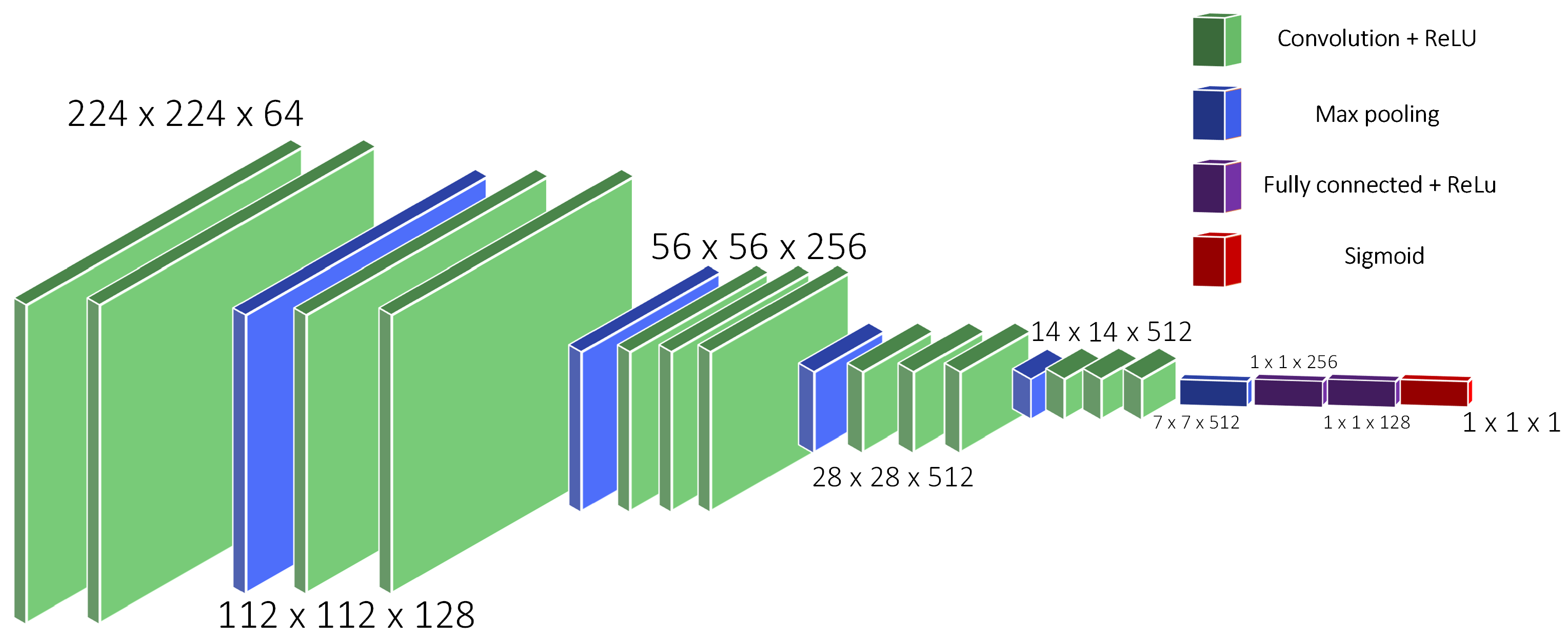
An important task to be completed before starting the lung images’ analysis is the selection of the CT slices, which include lungs, out of all the set of slices obtained from the multi-slice CT. In our system, for this purpose, we decided to use two of the neural network tested in [14], i.e., VGG16 and VGG19.The structure of the VGG16 network is presented in Figure 2.
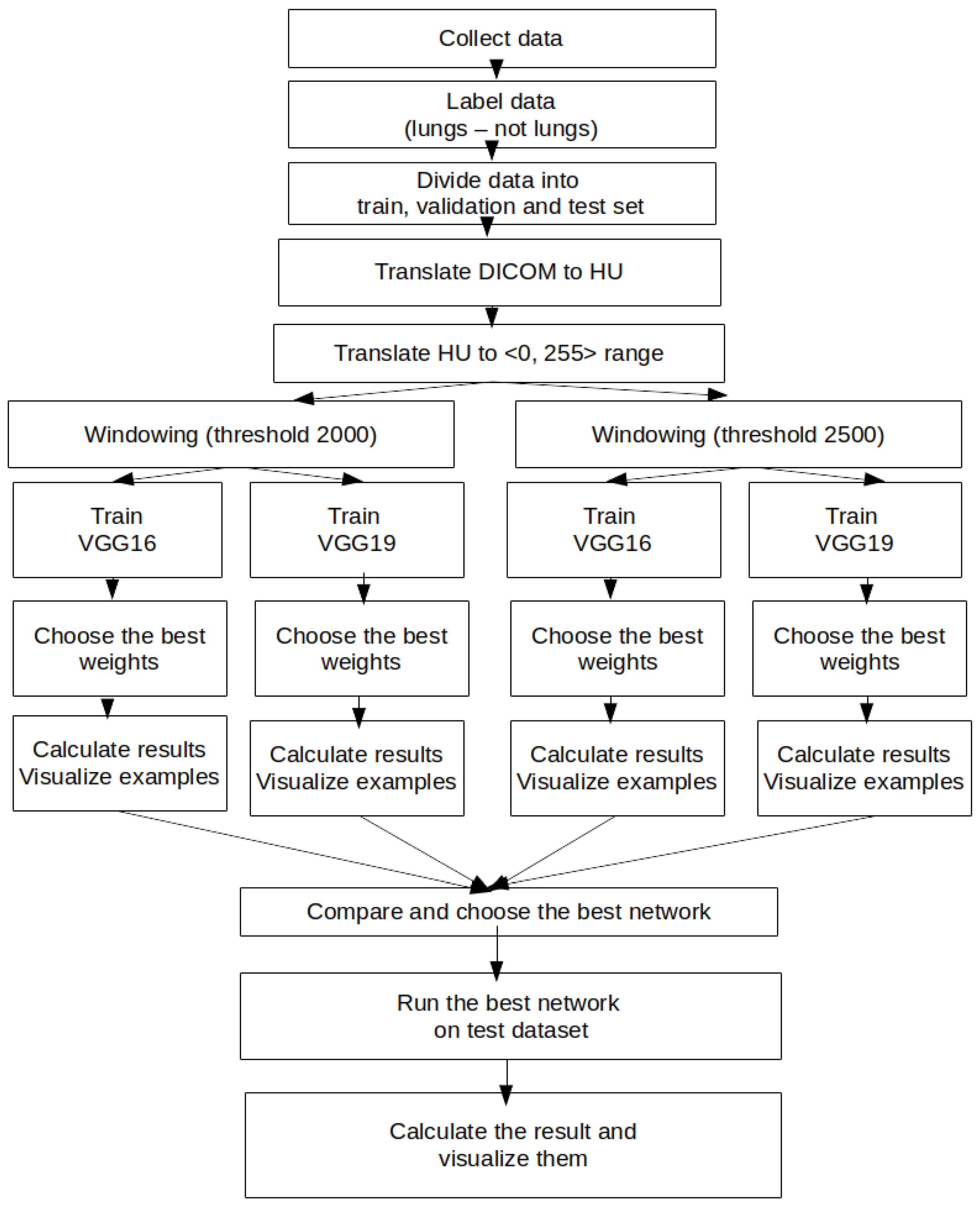
The data flow of the implemented procedure is presented in Figure 3.
The input data required for CNN training, validation, and testing were downloaded from the Cancer Imaging Archive website [15]. The selection filter was set to the following values:
  • Collections: NSCLC-radiomics
  • Image modality: CT
  • Anatomical site: lung
The structure of the training, validation and testing data is described in Table 2.
After reading the slices given in DICOM, the necessary scaling was applied. First the read slices were converted to the Hounsfield scale. The minimum threshold was set to −1024 (−1000 is the air level). This operation reset the PixelPaddingValue parameter, which was present in some DICOM files. The next operation moved the scale to include only positive values (simply a minimum value in each slice was added). Next, the maximum threshold was set. All values above X were changed to X (X = 2000, 2500). The resulting range was rescaled to real numbers in the range <0.0, 1.0>. Since the VGG network was designed for RGB input images, we tripled the one input channel. It was also necessary to change the slice image size to 224 × 224. We used a sigmoid activation function for the last layer in the VGG networks and the ReLU (rectified linear unit) function for the other layers. The padding parameter was set to same value, and the training process was set for 32 epochs.
As mentioned above, we tested two sets of input data with different maximum thresholds X (X = 2000, 2500) and two CNN configurations: VGG16 and VGG19. We also set the threshold imposed on the CNN’s output to 0.5 in order to obtain two responses: not lung and lung. The confusion matrices for the validation set are presented in Table 3. In order to be able to compare the performance of the tested networks, sensitivity and specificity were calculated on the same data; they are presented in Table 4.
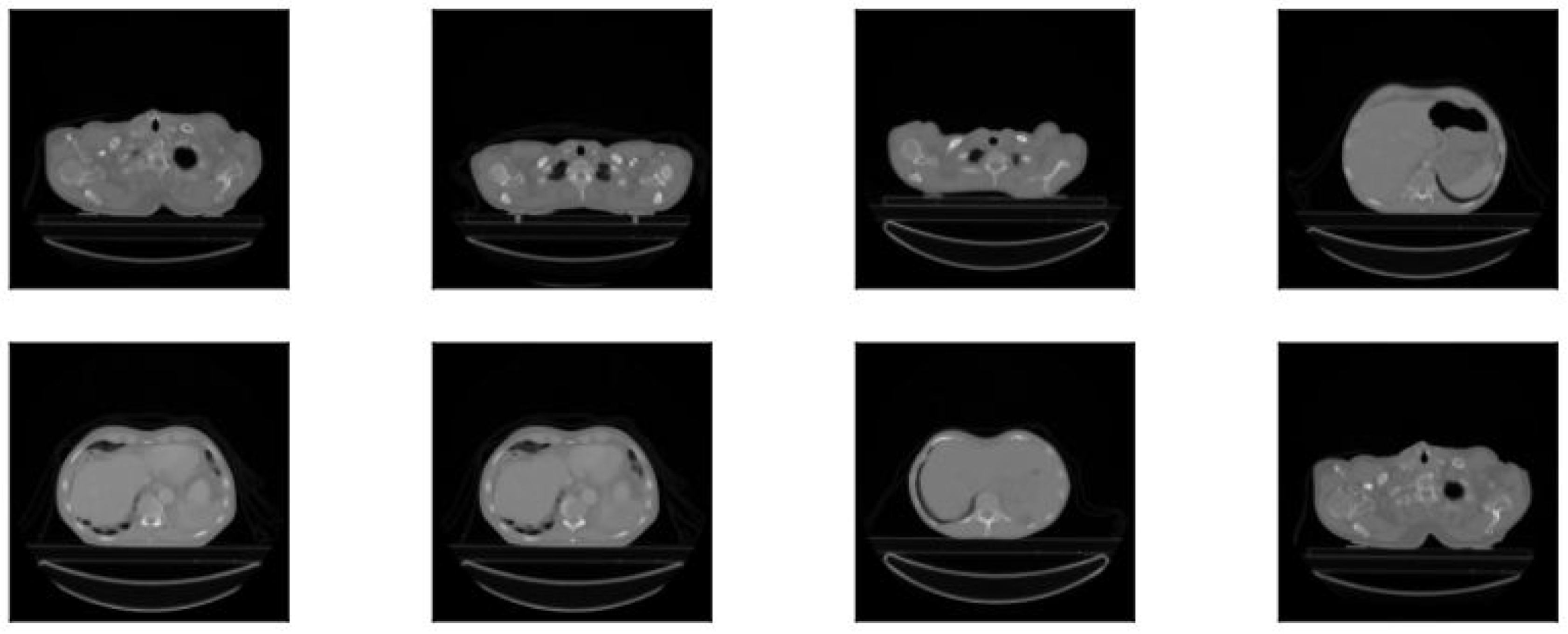
VGG16-2500 was discarded because of not lung images being classified as lung. These mistakes did not appear for the other networks, which in fact were similar in accuracy. We noticed a difference for 1–2 images; however, in these cases, the expert’s decisions for the validation sets were also not clear. Figure 4 illustrates the set of images that were classified by all tested networks as FN, which means the image was classified as not lung, whereas it contained a lung.
Figure 5 illustrates the set of images that were classified by all tested networks as FP, which means the image was classified as lung, whereas during labeling, a clinician decided there was no lung. It can be seen that in that case, the clinician made a mistake, because we can find a small part of a lung in each image.
Finally, VGG16-2000 was chosen because of the slightly better results. The achieved results on the testing set are presented in Table 5.

4. Lung Images’ Segmentation and Registration

4.1. Segmentation Process

In order to extract the examined region of interest (ROI) areas from whole images, the segmentation process is necessary. According to [16], lung segmentation may be challenging, because there are differences in pulmonary inflation, which can lead to large variability in volumes and margins when trying to implement automatic algorithms. There is still no universal segmentation method that will properly work for all lung pathological conditions. The amount of unique lung disease cases makes accurate segmentation without human verification very difficult. We can group traditional segmentation methods into fourmain categories: thresholding-based, region-based, shape-based, and neighboring anatomy-guided [16]. We will focus on the first two approaches, i.e., thresholding-based and region-based, which were used in our system. It is important to note that usually to achieve a properly segmented image, multiple techniques are combined.

4.1.1. Thresholding-Based Segmentation

The most basic and easy to implement is a thresholding-based method. We can set a certain global threshold value for the whole gray-scale image. The picture will be transformed into a binary region map, with ones where pixel values are above or equal to the threshold level and zeroes where they are below. Although the algorithm is simple, the most difficult step is to automatically find the threshold level for a specific image. Having lung CT images taken by different machines, the values of pixels representing lungs may differ. Generating a histogram from an image can help to choose the threshold values.
Unfortunately, even choosing a proper threshold does not guarantee that the desired object will be acceptably segmented. Sometimes, images have different lightning in different areas, and applying a simple threshold would give unacceptable results. That is why an adaptive threshold algorithm was introduced. It calculates the threshold “adaptively” for each region of an image. Thanks to this solution, the output is more accurate. It takes into consideration the different brightness of the pixels of the same object, which may be caused by lightning or a faulty camera [17]. The main advantages of this method are the calculation speed and simplicity of implementation. However, it works efficiently only when there is a large contrast between separated objects (which usually is not true in the case of lung CT images). It is very difficult to obtain a satisfying result if there is no significant value difference in the gray levels [18,19].

4.1.2. Region-Based Segmentation

Another approach to lung segmentation includes region-based methods. The most popular from this group is a region-growing algorithm. In general, it compares each pixel to its neighbors, and if a certain condition is met, it is added to the chosen region. One of the main algorithms representing this technique is region-growing. It uses the technique of pixel connectivity as described in [19]. This method segments the whole image into smaller regions, based on the growing (manually or automatically) of the chosen initial pixels (seeds) [17]. The algorithm begins at the initial pixel and checks whether its neighbors are within the threshold range given as an input parameter. If yes and the pixel does not belong to any other region, it is marked as visited, and all pixels from the neighborhood are recurrently checked. When a region is labeled (there are no pixels within the threshold in the neighborhood), a new starting point is chosen, and the algorithm begins to search for another connected region [20]. The main idea is to have pixels with similar properties located together within a region. Compared to simple thresholding, the computational cost of this solution is greater [18]. However, due to taking into consideration the spacial information and region criteria, these methods can conduct lung segmentation much more efficiently and with higher accuracy than the thresholding-based ones.
Another region-based algorithm is split-and-merge. At the beginning, the whole image is treated as a single region. Next, it is iteratively split into smaller sub-regions, until no further splitting is necessary. After that, similar regions are merged together, and a new one is created [17]. The stopping condition of the algorithm is reaching the expected number of regions given as the input or region uniformity. The split-and-merge algorithms are often implemented employing a quadtree data structure [21]. This approach overcomes the need for choosing initial seed points. Unfortunately, it is computationally expensive, because it requires building a pyramidal grid structure of the image [22].
The solution that was a starting point in the approach used in our system is called the watershed transform. The whole image can be treated as a surface. High insensitivity pixels correspond to peaks and low to craters. An intuitive example with a description can be found in [23]. The main goal is to identify the center of each crater—the local minimum called the marker. They give us an approximate idea of where different objects can be possibly located. Each marker is at the bottom of a unique basin, and the algorithm starts filling these basins with different colors, until reaching the boundary (the watershed line) of the adjacent marker [17]. This algorithm was implemented and tested in our system for lung segmentation.
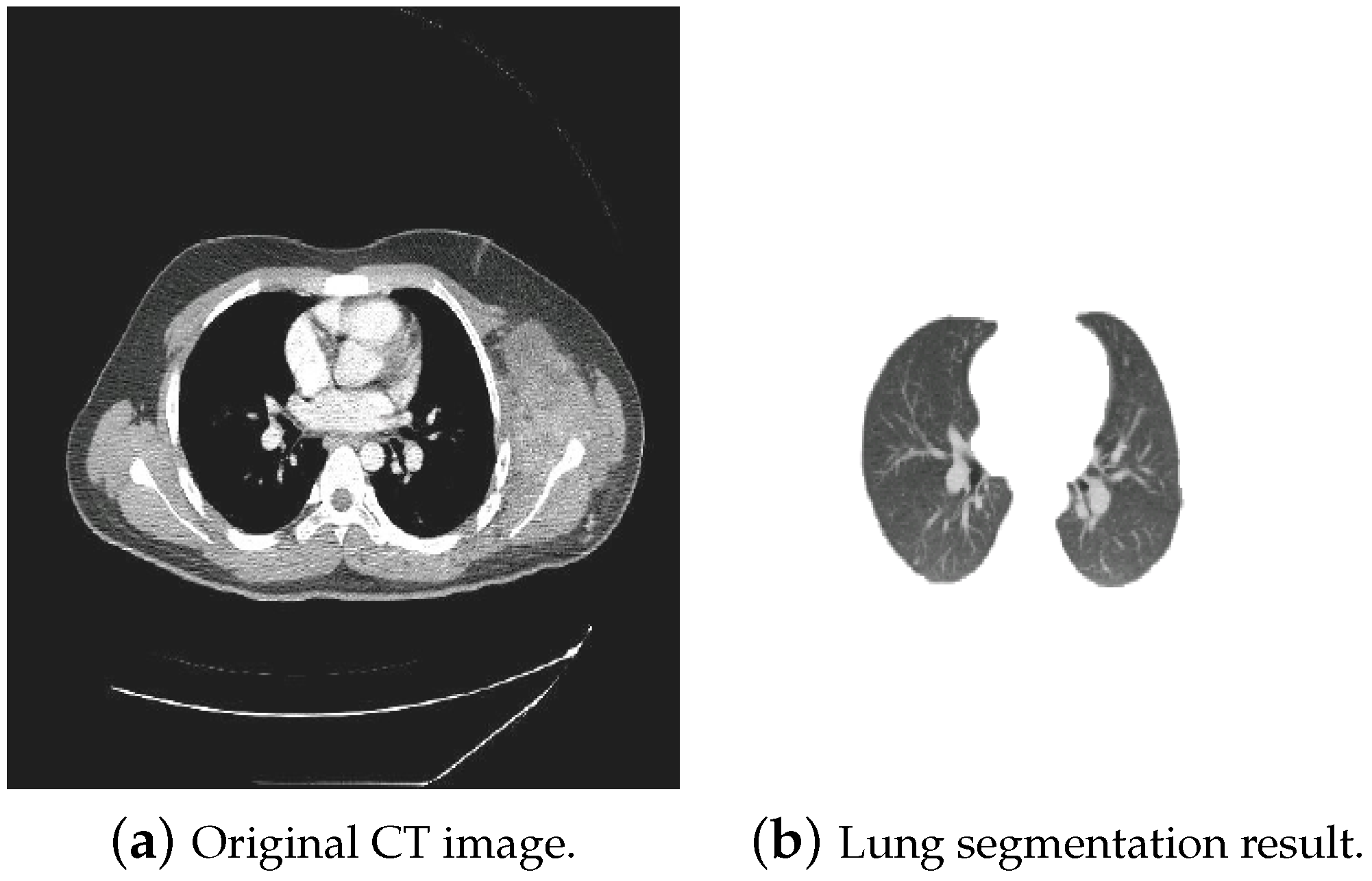
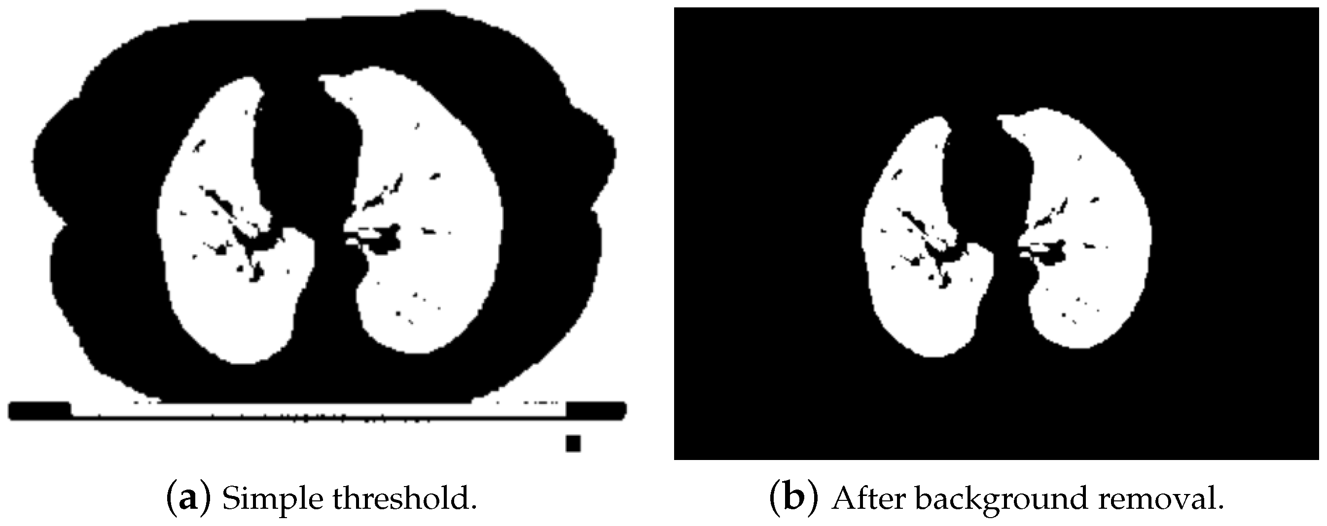
A possible problem of this approach is a lung oversegmentation. This occurs because each regional minimum forms its own small basin, which will be later filled while applying the transform. To overcome this problem, in [24], an extended version of the watershed transform was proposed. Region minima are decreased and next bounded within the region of interest in order to prevent oversegmentation. Choosing internal markers is the key step of this approach. In the described solution, these markers are connected components of pixels that have similar intensity values (in Hounsfield units (HUs)) and whose external boundary pixel values are above a certain gray level. According to [25], the lung region is in the range from −600 HU to −400 HU. That is why to specify internal markers, only pixels with a value lower than −400 are chosen. After eliminating the background, applying morphological transforms, imposing regional minima, applying the watershed transform, and filling the cavities, the segmented lung regions are obtained (Figure 6).

4.2. Registration Process

Image registration is used to overlay multiple images of the same object or scene taken at different times with the use of the same or different devices [26]. It is used in different fields such as medicine, remote sensing (e.g., environmental monitoring, weather forecasting), cartography, and computer vision. Usually, some preprocessing steps like noise removal, normalizing image sizes, or smoothing filters are applied. As described in [27], medical image registration is an integration process applied in order to bring images acquired from different modalities into spatial alignment. An example of registration usage is radiotherapy treatment planning. Doctors can merge images from different devices and/or different times and prepare a proper dosing plan.
A survey of pulmonary image registration methods was given in [28], and it discussed the following approaches:
  • Intensity based—registration relies on statistical criteria for matching different intensities between fixed and moving images.
  • Feature based—registration is based on different geometrical structures, i.e., points or curves, very useful while registering pathological lungs.
  • Segmentation based—in rigid registration, the same structures from both images are extracted; after that, they become the input parameters for the main registration method; unfortunately, registration accuracy is connected with the segmentation quality.
  • Mass-preserving—registration relies on detecting density changes on CT images, which are related to different inhalation volumes (air volume in lungs).

5. System Implementation

Python was chosen as the programming language for this project. An important factor for this choice was the availability of many well-documented image processing libraries (e.g., scikit-image, SimpleITK, OpenCV). The syntax and simplicity of writing the code were additional arguments.
Our input data were two CT images series. The first one was taken before radiotherapy (RT), and the second one was acquired during the follow-up. Different CT devices were used during the examinations, and the obtained CT series had different size parameters. Images that were taken before RT had a slice thickness equal to 3 mm, whereas the later images had this value at the level of 1.25 mm. For further processing steps (segmentation, registration, calculations), we had to equalize the number of slices in both series, trying to choose the closest corresponding slices. The first tested approach was based on the slice thickness. We assumed that the first slices from both series were corresponding ones. This could be done because we selected the corresponding beginning and ending slices in both series. Next, we prepared a table where each slice (from both series) had its relative distance to the beginning one. Finally, we iterated over each slice from the “before” series, taking its relative distance and finding corresponding slice from the “after” series, where the difference between those relative distances was minimal. Having selected slices with lung images (this was done using the CNN network described in Section 3), the next implemented block was responsible for the segmentation.

5.1. Segmentation

5.1.1. Watershed Segmentation

The watershed lung segmentation algorithm was based on the solution described in [24], but in order to achieve a satisfying result, many additional operations were added. Finally, our watershed transform segmentation had the following structure:
  • The first step was aimed at finding internal labels. The threshold filter at the level of −360 HU was applied in order to distinguish lungs. Obviously, as presented in Figure 7a, after thresholding, we obtained not only lungs, but also other elements, e.g., the background, pixel intensity of which was at the level of −1000 HU. In order to remove the background, a clear_border function from the skiimage.segmentation module was used. Thanks to that, only lung pixels were left, as shown in Figure 7b.
    Afterwards a labeling function from the scikit.measure package was used, in order to mark pixels that belonged to the same groups with unique labels. Unfortunately, this solution worked well only for the slices from the middle part of the series. The first ones contained organs like trachea or other significant airways, which were also detected using the threshold (due to the air inside them; a similar Hounsfield value), as shown in Figure 8. In further steps, these areas could be mistakenly treated as internal markers.
    To solve this problem for the first 9% of the slices (which very likely contained trachea), additional steps were implemented in order to properly detect only lungs.
    • All regions with areas smaller than 0.00012 of the whole image size were removed. This was necessary in order to get rid of noise and very small insignificant objects, but at the same time, this value cannot be too high, because it would reject regions with small sections of lungs (beginning slices). As a result of this step, we were able obtain two or three segmented regions.
    • If only two regions were left, that meant that one of them was lung, and the other was trachea. We could assume that due to the fact that in all images containing lungs, lungs were bigger than trachea. We found the minimum y value of pixels in both areas (located at the top of each area) and removed this region, which had the smaller value (trachea is above lungs on the first slices). This analysis is illustrated in Figure 9.
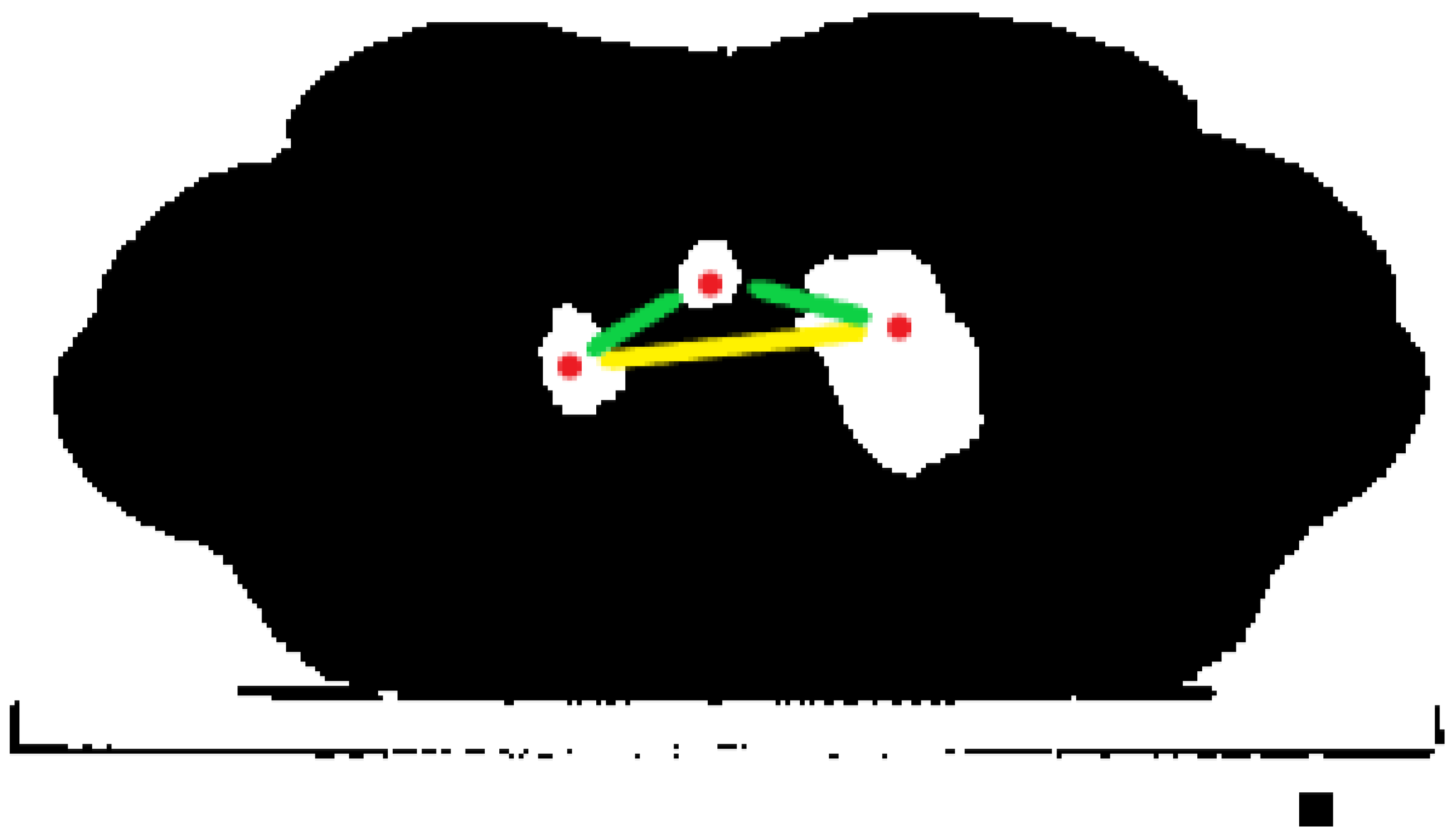
    • If in one of the first slices, three regions were detected, that meant that two of them were lungs, and one was trachea. Unfortunately, we could not simply preserve the two largest ones, because we were not able to ensure that lungs were bigger than trachea (usually, it is the opposite). That is why for this purpose, we detected the centroids of each region (they had x and y coordinates). Next, we made a list of all possible pairs of centroids and calculated the Euclidean distance between each pair. As a result, we obtained a list of three distances, sorted them, and kept the two regions between which the distance was largest. A simple visualization is shown in Figure 10.
  • The next step was finding external labels. This was done by dilating the internal marker, creating two temporary matrices, and taking regions where they were different from each other (XOR operation). By changing the dilation iterations, we were able to control the distance between those two markers. The external marker looked like a wide border surrounding the internal one. The border had to be wide enough to cover all minima, which could be located in the neighborhood. The final watershed marker containing internal and external ones is presented in Figure 11.
  • Afterwards, the Sobel filter along both axes (x and y) was applied in order to detect edges on the input image (Figure 11).
  • The watershed algorithm was executed with the sobel_gradient and watershed_ markers as inputs. In order to find the border of the result of the watershed algorithm, morphological_gradient was applied (with the difference between the dilation and erosion of the watershed as the input). In order to re-include significant nodules near the border, a black-hat operation was applied. Thanks to that, the areas that might carry significant information about the treatment were still in the segmented lungs. We decided that it was better to include an area that normally would not be treated as lung in the segmentation process. If we wanted to omit it during the calculations, we would just contour it with an ROI and exclude it from the calculation area. Removing it during segmentation would lead to a loss of the significant information that it carried.
  • Finally, binary opening, closing, and then, small erosion operations were applied in order to remove noise and fill the holes, which were inside lungs after thresholding. Examples of segmented lungs are presented in Figure 12.
The total time of segmenting both series was 50.7 s.
Obviously, in order to make this algorithm more universal and able to segment a larger amount of different lung series, we would probably omit the step of detecting trachea on the first slices and simply remove objects that have a larger ratio. Unfortunately, small lung areas on the beginning slices would not be detected, but if we conducted the calculations on a big amount of patients (100–150), then this would become less significant.

5.1.2. Segmentation Using the SITK Library

The watershed algorithm segmented lungs quite properly, although sometimes, especially for the first or last slices, the resulting masks were too sharp. Lung borders should be smooth in order to properly reflect the reality. At the same time, such segmented lungs would be easier to register. The second approach was implemented using the SimpleITK (SITK) library and based on the example described in [29]. Below, we give the steps of the SITK segmentation algorithm:
  • In order to denoise and smooth the image, we used a CurvatureFlow image filter. Smoothed images are better for further processing.
  • In order to separate lungs from the background and other organs, a threshold value at −280 HU was set. It does not strictly correspond to the theoretical Hounsfield range of lungs (form −400 to −600 HU), but the acquired images came from different modalities, so we wanted to cover all lung areas, with pixels in a close neighborhood.
  • The next challenge was to remove the background. We decided to use a NeighborhoodConneted function. It labeled pixels connected to an initially selected seed and checked if all pixel neighbors were within the threshold range. The initial seed was chosen as point (10, 10), which was located near the upper left image corner. Pixels with a value equal to zero in the thresholded image (background) were set to one. In the thresholded image, pixels containing body parts other than lungs were also set to one. Adding a thresholded image to the neighborhood connected one gave us a result with segmented lungs and some noise. In Figure 13, the first segmentation steps are depicted.
  • After detecting lungs, a ConnectedComponents filter was applied to label the object on the input binary image. Pixels equal to zero were labeled as background, whereas those equal to one were treated as objects. Different groups of connected pixels were labeled with unique labels.
  • In the next step, the area of detected objects was calculated, and the largest one or two, whose size was larger than 0.002 of the whole image, were chosen. Due to this condition, right lung in the third slice was not detected by this algorithm, but it was in the watershed. In order to fix this issue, additional restrictions for the extreme slices should be added.
  • On such a segmented lung binary image, opening and closing were applied. Binary opening was responsible for removing small structures (smaller than the radius) from the image. It consisted of two functions executed on the output of each other: Dilatation(Erosion(image)). On the other hand, binary closing removed small holes present in the image.
  • Sometimes, after applying those filters, still, some large holes were left inside the images. Usually, they should stay there, because the area did not match the conditions. However, in our lung segmentation approach, there should not be any holes left inside the lung area. In order to satisfy this requirement, a VotingBinaryHoleFilling filter was applied. It also filled in holes and other cavities. The voting operation on each pixel was applied. If the result was positive, it was set to one. We chose a large radius for this operation (16) in order to ensure that no holes would be left inside.
  • Finally, we applied a small erosion filter with the radius set to one. We excluded the lung border from the segmented image. Tissue located in that area was irrelevant for the analysis and could even falsify the results.
Although this approach gave slightly better results, when it came to the final lung segmented shapes, still, some additional filters or methods should be added in order to make this algorithm more universal. Some of the last slices (Figure 14) were segmented more accurately, but the time of calculations—218.6 s for both series—were much longer than for the watershed algorithm—50.7 s.

5.2. Registration

The registration process started with an affine registration where transformations like rotation, scaling, and translation were used. The results of the affine registration were supposed to give a better initial step for further elastic registration.

5.2.1. Affine Slice Registration

Firstly, we analyzed the whole previously segmented images not as solid 3D figures, but as individual slices. Each pair of corresponding slices was registered, where the image from the after series was treated as moving_image and the one from the before series as fixed_image. For this task, we also used the SITK library [30]. Before executing the registration algorithm, many parameters had to be specified:
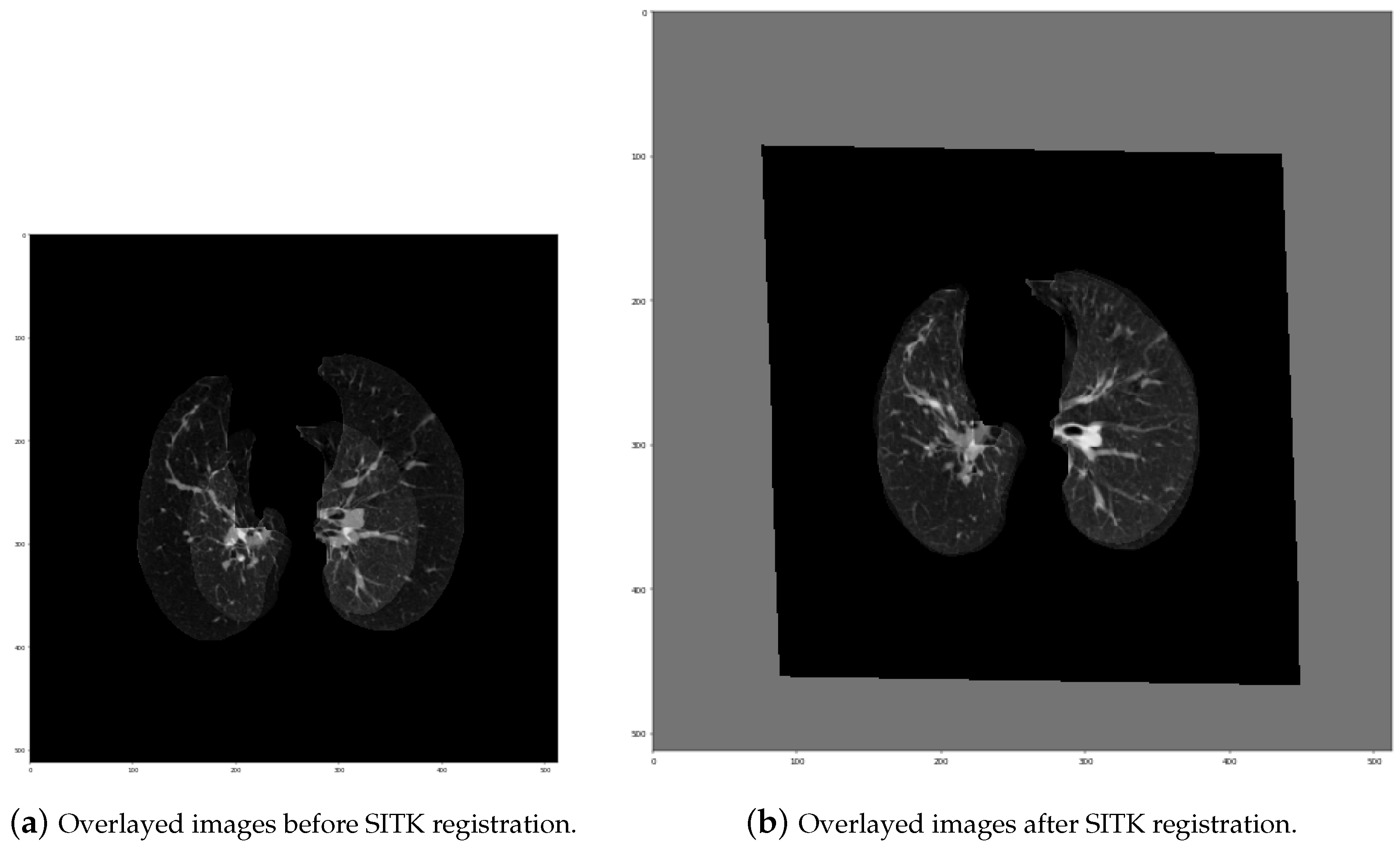
  • Initial transformation: In this step, we used CenteredTransformInitializer in order to align the centers of both slices. At the same time, the AffineTransform transformation type was chosen. Transformations like Euler2DTransform would not be proper in this case, because both series were acquired by different devices, which means they had various scales. Euler transformation is specified as rotation and translation, but without scaling. As seen in Figure 15, lungs on the “before” series were much smaller those on the “after” series, so scaling was one of the most significant needed transformations.
  • Measure metric: We used MattesMutualInformation. The metric sampling strategy was set to REGULAR, and the metric sampling percent was set to 100%. That means that to calculate the current measure, all pixels were taken into consideration. Due to the fact that lung segmentation was performed before registration, we could not compute the metric using a small percent of random points, as was proposed in [31]. If only black points (outside the lungs) had been randomly chosen from both images, then the cost function would have been very low, but it would not mean that the lungs were properly registered.
  • Interpolator: We set it as Linear. In most cases, linear interpolation is the default setting. It gives a weighted average of surrounding voxels with the usage of distances as weights.
  • Optimizer: The gradient descent optimizer was chosen for affine registration. It has many parameters to be set, and we used the following:
    • learningRate = 1,
    • numberOfIterations = 255.
  • Multi-resolution framework: The last set parameters were associated with the multi-resolution framework, which the SITK library provides. Due to this strategy, we were able to improve the robustness and the capture range of the registration process. The input image was firstly significantly smoothed and had a low resolution. Then, during the next iterations, it became less smoothed, and the resolution increased. This additional multi-resolution utility was realized with two functions: SetShrinkFactorsPerLevel (shrink factors applied at the change of level) and SetSmoothingSigmasPerLevel (smoothing sigmas applied also at the change of level—in voxels or physical units). In affine registration, where the images differed significantly from each other, we decided to set four multi-resolution levels. The chosen parameters were as follows:
    • shrinkFactors = [6,4,2,1],
    • smoothingSigmas = [3,2,1,0].
We executed this algorithm for each pair of corresponding slices. An example of an image before and after affine transformation is shown in Figure 16. The time of affine registration for one slice was 2.5 s, and the total time of affine registration for the whole series was 168.1 s.
Table 6 presents the SimpleITK “one slice” affine registration results.

5.2.2. SimpleITK 3D Affine Registration

Affine registration of the whole segmented and raw 3D images was also tested. We wanted to compare how the registration results and times of calculations depended on the input 3D image and chosen samplers (for the segmented image, we had to sample all points, not only those randomly chosen). In order to test how the SimpleITK library handles 3D image registration, we implemented two short programs. The first one was prepared for registering raw CT images, and the second one was responsible for registering lungs segmented from those images. As expected, it took longer to register 3D images with previously segmented lungs than the raw ones. Table 7 compares the results of the 3D affine registration using SimpleITK. In Figure 17, overlayed raw slices, before (a) and after (b) affine registration, are depicted. In order to visualize the differences in registration between raw and segmented images, Figure 18 presents overlayed segmented slices also before (a) and after (b) affine registration. As seen when it comes to 3D registration, the slices, from the middle of the series, are transformed properly.

5.2.3. Elastic Lung Registration

Another approach to the registration, implemented in our system, was the elastic registration. This algorithm was implemented using two libraries: SimpleITK and SimpleElastix. It needs to be noted that elastic registration is much slower and more sophisticated than affine. As seen in Figure 16, the first registration step gives quite satisfying results, so the elastic registration will not need to start the process from scratch. Many parameters are similar to those from the affine registration process, so below, we present only the chosen ones, which are different:
  • Initial transformation: In this step, we chose the BSplineTransformation type.
  • Measure metric: It is analogous to the affine one.
  • Interpolator: It was also set as Linear.
  • Optimizer: The gradient descent optimizer was also chosen for elastic registration; however, its parameters slightly changed:
    • learningRate = 1,
    • numberOfIterations = 255.
  • Multi-resolution framework: The parameters of the multi-resolution framework were also changed:
    • shrinkFactors = [2,1],
    • smoothingSigmas = [1,0].
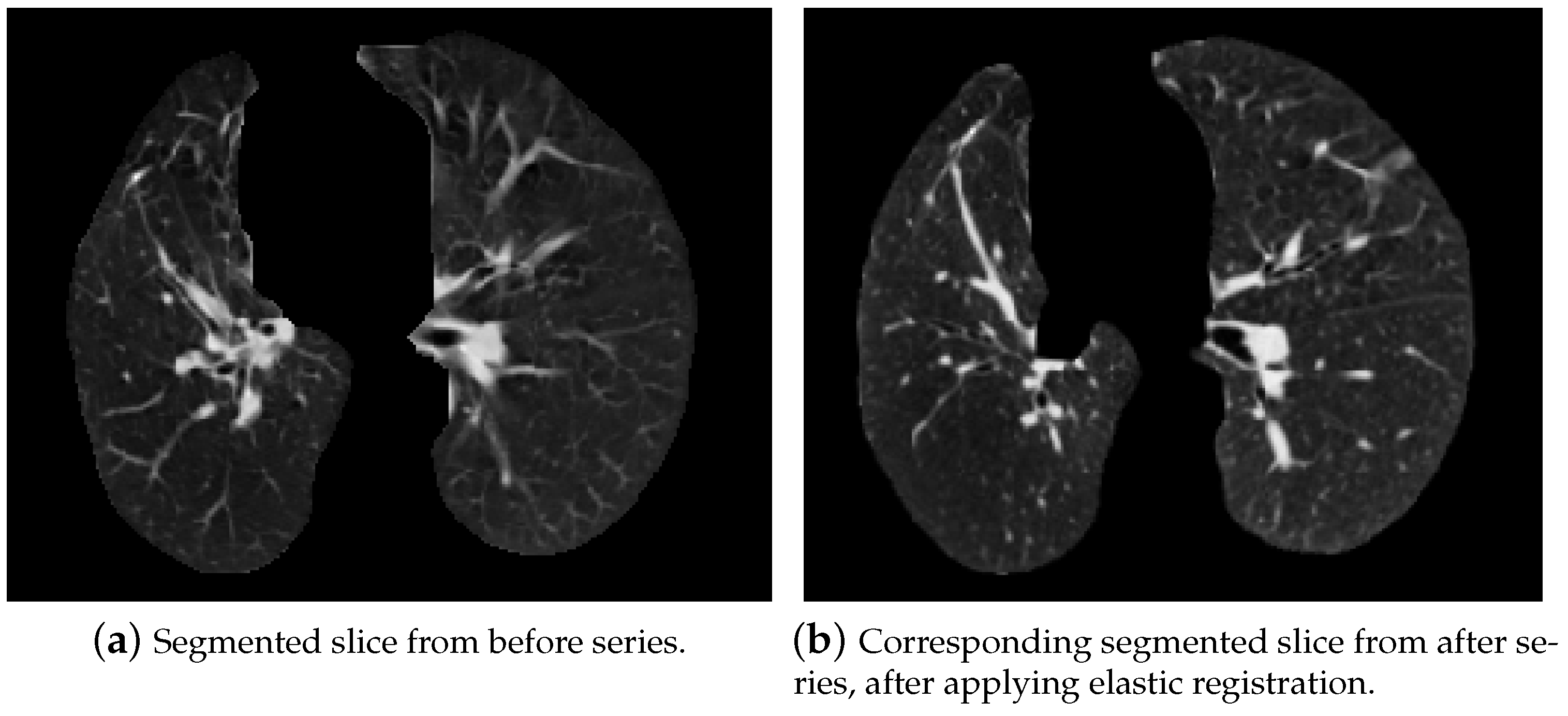
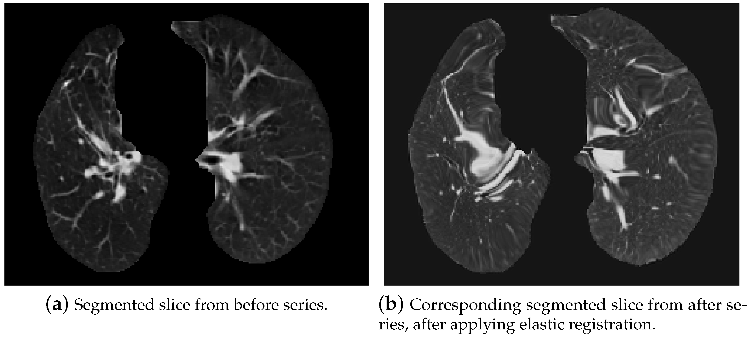
The elastic registration algorithm was also executed for each pair of corresponding slices, where the moving slice was the one after affine registration, and the fixed one was invariably the segmented slice from the “before” series. An example of an image before and after elastic transformation is shown in Figure 19. The time of elastic registration for the whole series was 2103.4 s. Table 8 presents the SimpleITK “one slice” elastic registration results.
In order to compare different implementations, the registration using the SimpleElastix library was also applied. It was also run for a pair of corresponding slices, where the moving slice was the one from the “after” series and the fixed one was the segmented slice from the “before” series. An example of an image before and after registration is shown in Figure 20.
Additionally, in order to evaluate the registration process, the SimpleElastix library gives the possibility to display the final metric (the AdvancedMattesMutualInformation metric was used) value. Table 9 presents the SimpleElastix “one slice” registration results.
Comparing these results with those presented in Figure 19, we can observe that these solutions differed from each other. Registering using SimpleITK did not change the lung structure significantly; however, at the same time, it did not make the images fully equivalent in terms of shape. The SimpleElastix approach preserved the shape better. Although SimpleElastix had a very good metric value (Table 9), we are not sure if the internal lung structure should be changed to such a large extent. Obviously, the parameters of the SimpleITK methods can also be changed in order to achieve results similar to those produced by SimpleElastix, but the calculation time increases dramatically.

5.3. Data Presentation Module

All aforementioned processing steps such as slice choosing, segmentation, and registration were conducted in order to finally obtain paired images of lungs with a similar shape so that “before” and “after” series can be compared slice-by-slice. Thanks to that, various statistics could be calculated on the corresponding images from the before and after series, including: the maximum, minimum, median, and mean of the pixels (in HU). This is necessary to compare subtle density changes that appear in different parts of lungs after radiotherapy and could be correlated with the delivered radiation dose and to assess the impact on healthy lung tissue. Some visualization functions were developed. The calculation methods were implemented based partly on the solutions presented in [29].
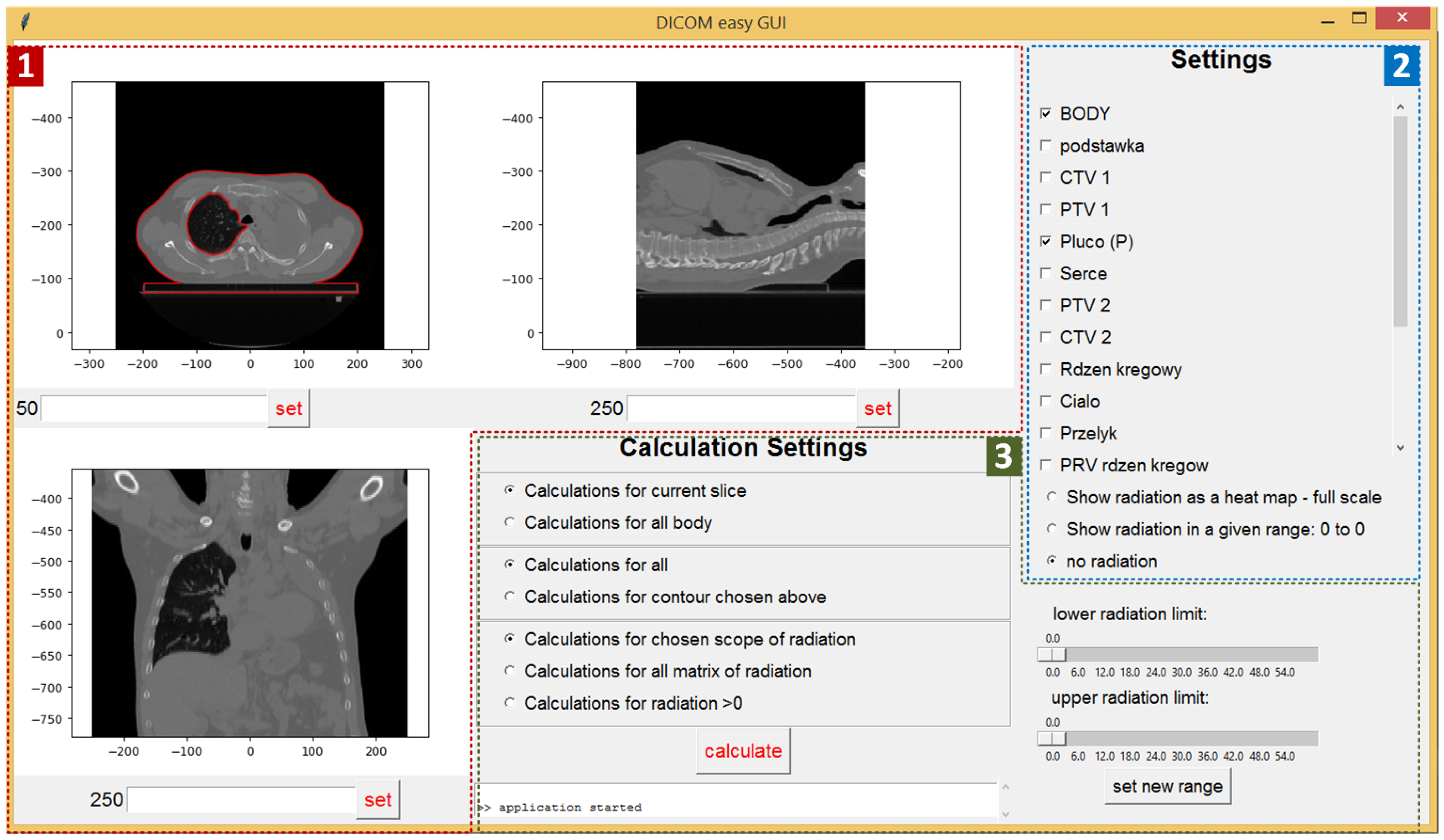
The main window of the system interface, presented in Figure 21, consists of three areas:
  • Current CT slice (displayed for three directions) (red area—1): The slice can be selected by setting its number or by using a mouse scroll wheel. By moving the mouse over the upper left slice, we can read the pointed pixel’s Hounsfield scale value and the dose density value in gray units. The small console at the bottom of the screen is used to display messages to the user (errors, warnings, etc.).
  • Input settings (blue area—2): Check boxes allow the selection of all contours loaded from the active files. Radio buttons are used to set the visible range of the radiation dose. There are three possible options:
    • Show radiation as a heat map (a “warmer” color corresponds to a higher radiation dose)
    • Show radiation in a given range (the range is set by the sliders located below)
    • No radiation (the CT slice is displayed without the radiation scheme).
  • Calculation parameters (green area—3): The first set of radio buttons specifies whether the results are calculated for the whole body (all slices) or just for the current slice. The second set of radio buttons decides whether the calculations are applied for all pixels or just for pixels within the chosen contour. The last three radio buttons are used to select the settings related to the radiation. Calculation can be done for the chosen radiation range (the scope is set by sliders), for all the matrix of radiation (for all pixels included in the radiation area), or for pixels where the radiation is above zero.
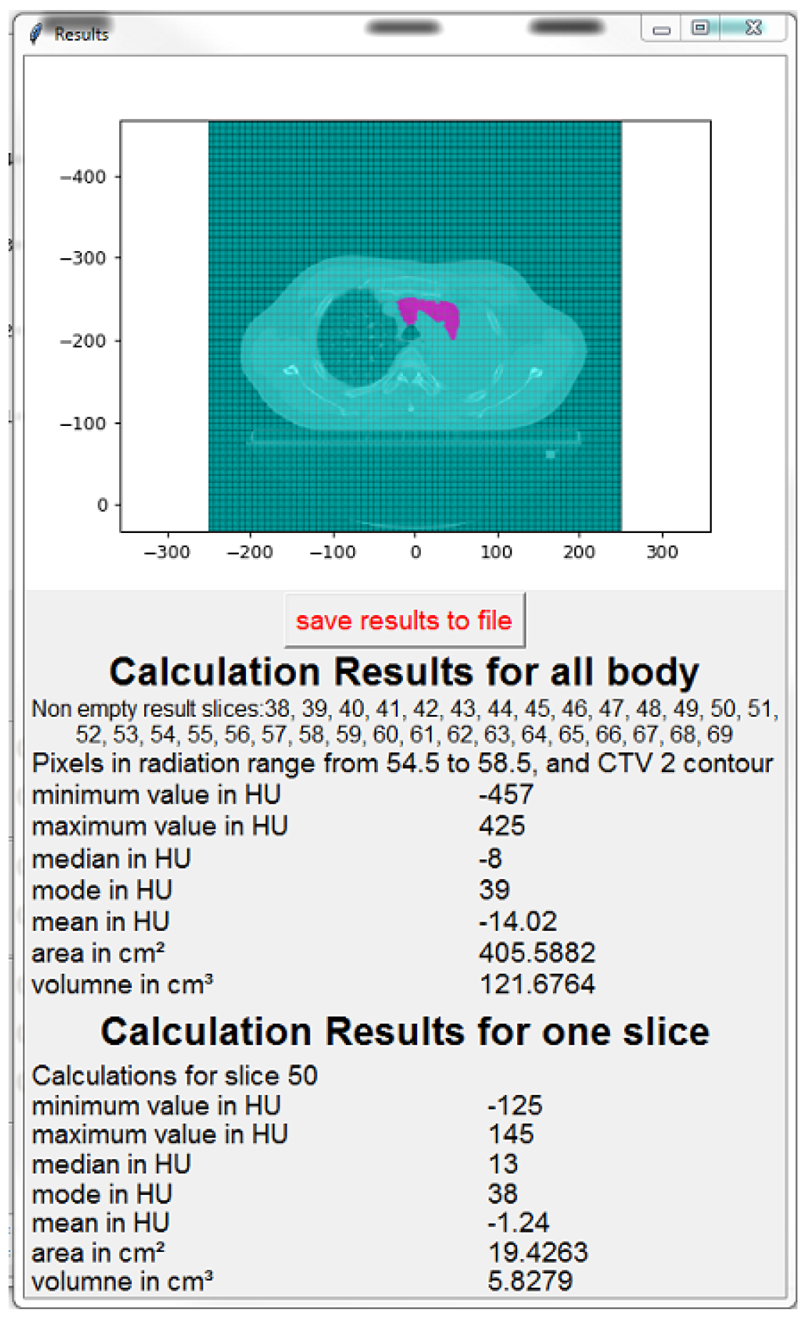
Clicking on the calculatebutton starts the calculations and generates the resulting window, presented in Figure 22. The reported results include:
  • The image of the current slice with marked pixels selected for calculation,
  • The number (indexes) of slices for which the calculation was done,
  • The calculation parameters (radiation range, contour type),
  • Min, max, median, mode, and average values in HU,
  • The volume and area of the selected pixels.
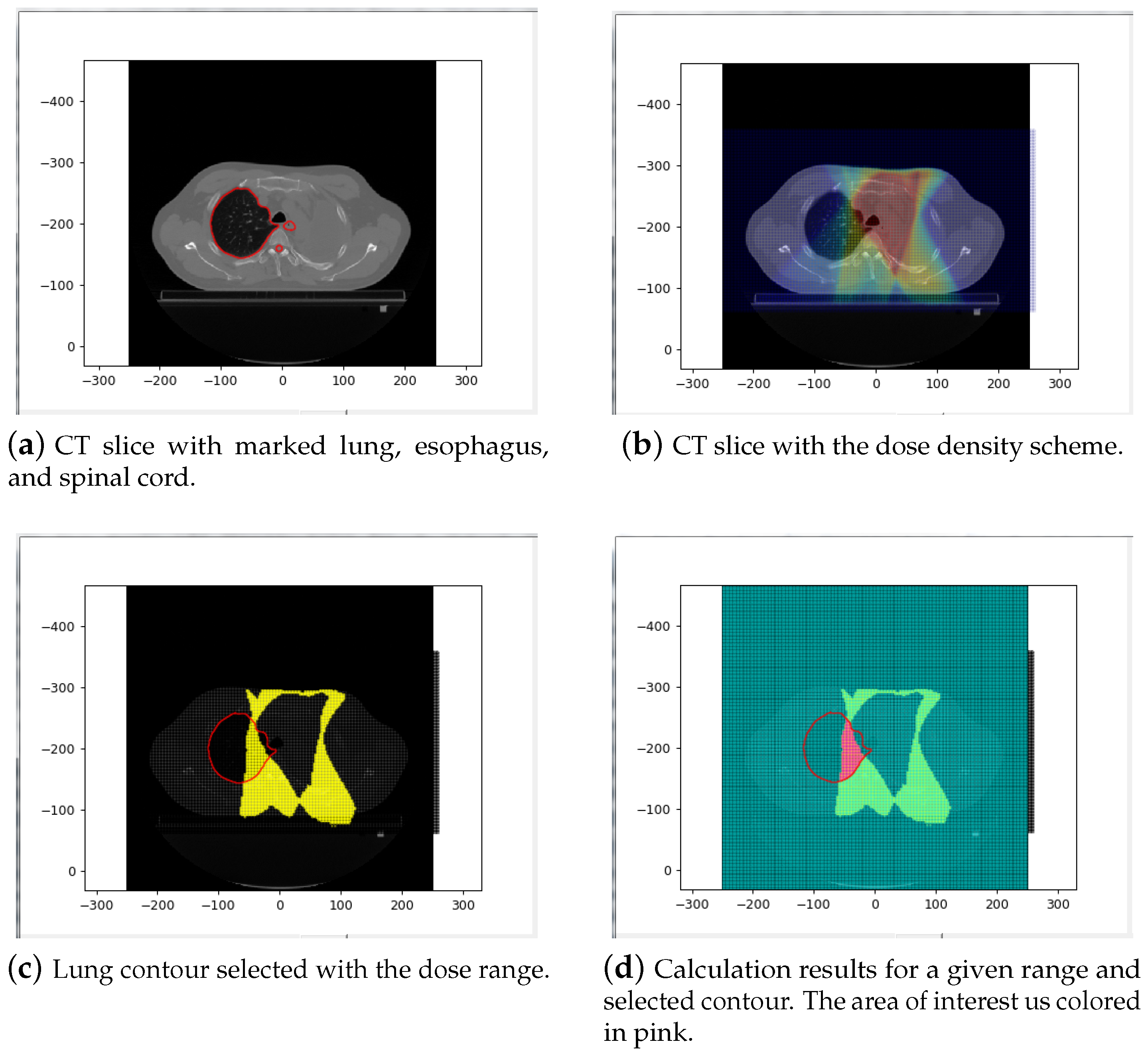
When the whole body option is chosen, it is possible to scroll through CT slices. Then, the calculation results are updated on-the-fly. Finally, the results can be visualized (Figure 23) and stored in a file. The first picture, shown in Figure 23a, shows the CT slice with marked lung, esophagus, and spinal cord, which is an input slice for further calculation. Next, Figure 23b presents a CT slice with the dose density scheme, Figure 23c the lung contour with the selected dose range, and Figure 23d the region of calculation, which is a cross-section of the segmented lung and the area of the selected dose range.

6. Conclusions and Future Works

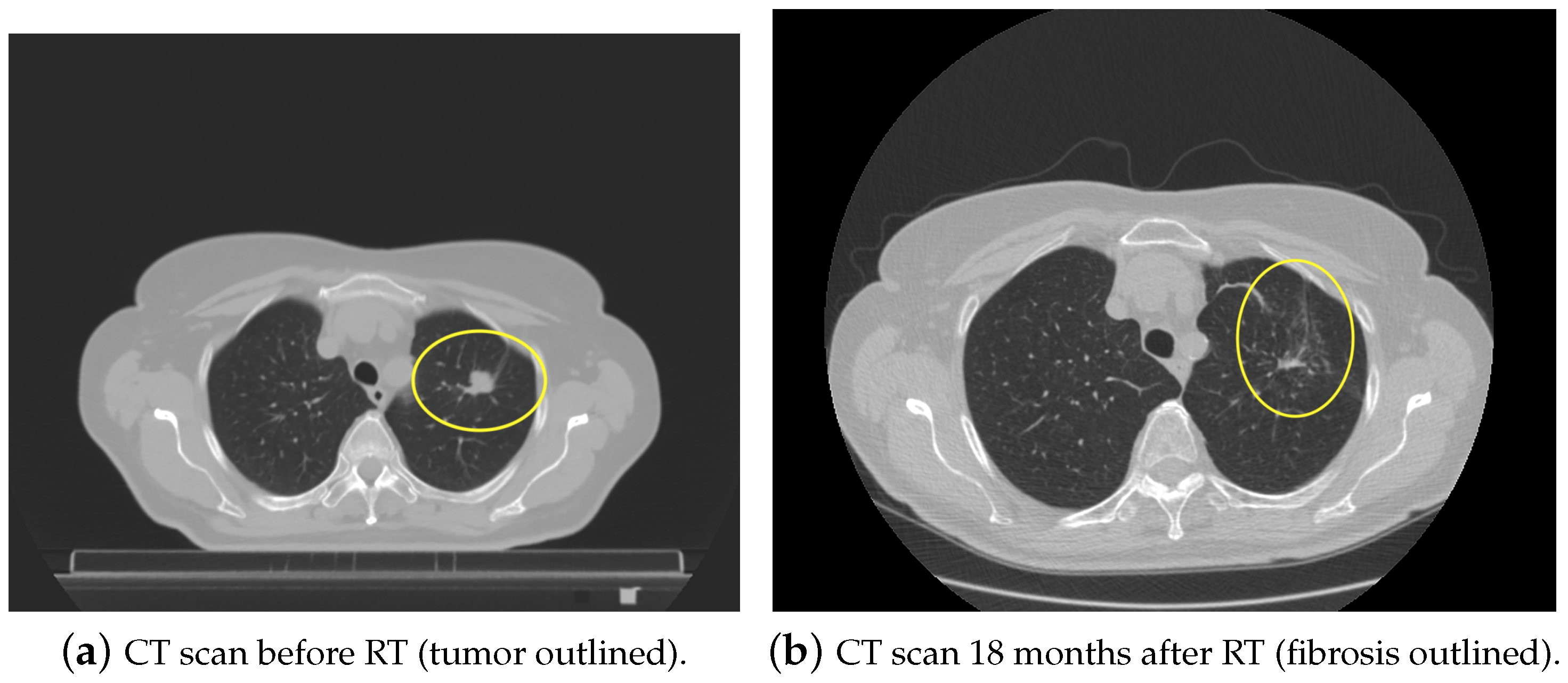
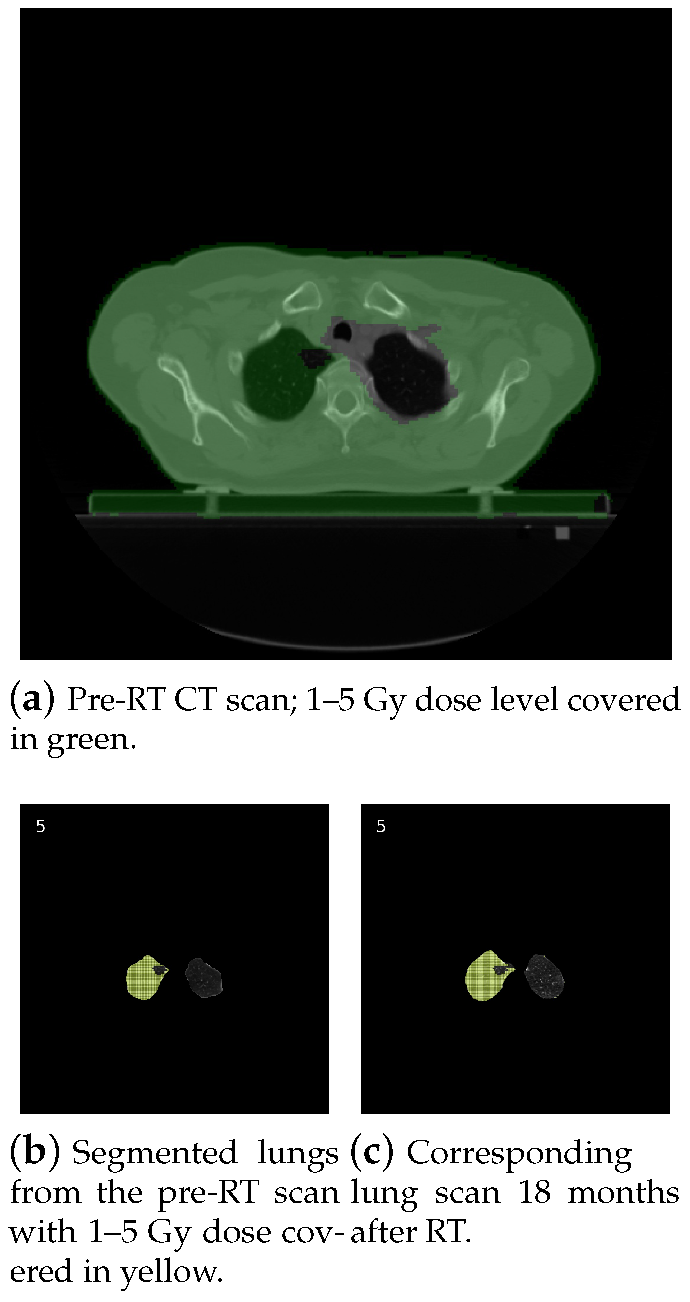
The paper presents a software tool that will be used for large-scale CT-based radiomics for radiation oncology specialists. This particular application is designed to analyze the correlation between the delivered dose and the density changes in pulmonary tissue, representing radiation-induced fibrosis. Currently, the tool is used for analyzing a big set of patients’ results, together with the clinical data, focusing on the impact of “low doses”—between 0 and 5 Gy. We presume that even these lowest doses affect the lung function and morphology over time as fibrosis develops even if it is not visible with the naked eye. As an example, in Figure 24, you can see the initial pretreatment image of the tumor and the 18 month follow-up scan with complete remission achieved. There is also an easily noticeable area of RILF that corresponds to the high doses delivered (40–66 Gy). However, it is difficult to see any density changes in other areas. Analyzing the precise density using our software, we find that mean HU values of the lung tissue where the 1–5 Gy dose was delivered during RT increased from −821 HU to −772 HU (Figure 25). Thanks to this, we hope to prove the statistically significant impact of low doses on a large number of patients.
The results can be important in the era of modern conformal radiotherapy methods, which decrease high dose levels in patient’s OARs at the cost of the, so-called, “low dose bath”. We aim to assess clinically useful dose constraints for conventional lung RT.
Apart from a numerical measurement of density changes, we will work on using AI solutions to analyze and predict the patterns and evolution of fibrotic changes over time. We also want to develop radiobiological concerns on hypofractionated regimens and new modalities like particle therapy. There is also a novel ultra-high dose rate FLASH-RTtechnique [32] that can decrease the lung toxicity [33]; however, this method is still in early pre-clinical studies. What is more, precise fibrosis analysis is also crucial for patients treated with modern immunotherapy, especially combined with conventional chemotherapy and radiotherapy being one of the most common toxicities. We should also remember COVID-19 patients and distinguish different CT abnormalities.

Author Contributions

Conceptualization: P.Ś. and M.K.; methodology: K.Ś., M.K., and B.B.; software: K.Ś. and B.B.; validation: K.Ś., M.K., B.B., and P.M.; formal analysis: S.W.; investigation: P.Ś., M.K., K.Ś., B.B., and S.W.; resources: P.Ś.; data curation: M.K. and P.Ś.; writing—original draft preparation: K.Ś., P.Ś., and M.K.; writing—review and editing: M.K., S.W., K.Ś., B.B., P.M., and P.Ś.; supervision: P.Ś.; funding acquisition: P.Ś. All authors read and agreed to the published version of the manuscript.

Funding

This research was funded by 0311/SBAD/0699 grants from Poznan University of Technology. The APC was funded by Poznan University of Technology.

Informed Consent Statement

Not applicable.

Acknowledgments

This work was partially supported by the 0311/SBAD/0699 grant from Poznan University of Technology, Institute of Computing Science.

Conflicts of Interest

The authors declare no conflict of interest.

References

  1. Ginneken, B.V.; Romeny, B.M.T.H.; Viergever, M.A. Computer-aided diagnosis in chest radiography: A survey. IEEE Trans. Med. Imaging 2001, 20, 1228–1241. [Google Scholar] [CrossRef] [PubMed] [Green Version]
  2. Wijsman, R.; Dankers, F.; Troost, E.G.; Hoffmann, A.L.; van der Heijden, E.H.; de Geus-Oei, L.F.; Bussink, J. Comparison of toxicity and outcome in advanced stage non-small cell lung cancer patients treated with intensity-modulated (chemo-) radiotherapy using IMRT or VMAT. Radiother. Oncol. 2017, 122, 295–299. [Google Scholar] [CrossRef]
  3. Wennberg, B.; Gagliardi, G.; Sundbom, L.; Svane, G.; Lind, P. Early response of lung in breast cancer irradiation: Radiologic density changes measured by CT and symptomatic radiation pneumonitis. Int. J. Radiat. Oncol. Biol. Phys. 2002, 52, 1196–1206. [Google Scholar] [CrossRef]
  4. Käsmann, L.; Dietrich, A.; Staab-Weijnitz, C.A.; Manapov, F.; Behr, J.; Rimner, A.; Jeremic, B.; Senan, S.; De Ruysscher, D.; Lauber, K.; et al. Radiation-induced lung toxicity–cellular and molecular mechanisms of pathogenesis, management, and literature review. Radiat. Oncol. 2020, 15, 214. [Google Scholar] [CrossRef] [PubMed]
  5. Warrick, J.H.; Bhalla, M.; Schabel, S.I.; Silver, R.M. High resolution computed tomography in early scleroderma lung disease. J. Rheumatol. 1991, 18, 1520–1528. [Google Scholar] [PubMed]
  6. Bernchou, U.; Schytte, T.; Bertelsen, A.; Bentzen, S.M.; Hansen, O.; Brink, C. Time evolution of regional CT density changes in normal lung after IMRT for NSCLC. Radiother. Oncol. 2013, 109, 89–94. [Google Scholar] [CrossRef] [PubMed]
  7. Mahmud, M.; Kaiser, M.S.; Hussain, A.; Vassanelli, S. Applications of Deep Learning and Reinforcement Learning to Biological Data. IEEE Trans. Neural Netw. Learn. Syst. 2018, 29, 2063–2079. [Google Scholar] [CrossRef] [PubMed] [Green Version]
  8. Song, Q.; Zhao, L.; Luo, X.; Dou, X. Using deep learning for classification of lung nodules on computed tomography images. J. Healthc. Eng. 2017, 2017, 8314740. [Google Scholar] [CrossRef] [PubMed] [Green Version]
  9. González, G.; Ash, S.Y.; Vegas-Sánchez-Ferrero, G.; Onieva Onieva, J.; Rahaghi, F.N.; Ross, J.C.; Díaz, A.; San José Estépar, R.; Washko, G.R. Disease Staging and Prognosis in Smokers Using Deep Learning in Chest Computed Tomography. Am. J. Respir. Crit. Care Med. 2018, 197, 193–203. [Google Scholar] [CrossRef] [PubMed]
  10. Kovács, A.; Palásti, P.; Veréb, D.; Bozsik, B.; Palkó, A.; Kincses, Z.T. The sensitivity and specificity of chest CT in the diagnosis of COVID-19. Eur. Radiol. 2020. [Google Scholar] [CrossRef] [PubMed]
  11. Zhou, L.; Li, Z.; Zhou, J.; Li, H.; Chen, Y.; Huang, Y.; Xie, D.; Zhao, L.; Fan, M.; Hashmi, S.; et al. A Rapid, Accurate and Machine-Agnostic Segmentation and Quantification Method for CT-Based COVID-19 Diagnosis. IEEE Trans. Med. Imaging 2020, 39, 2638–2652. [Google Scholar] [CrossRef]
  12. Luo, N.; Zhang, H.; Zhou, Y.; Kong, Z.; Sun, W.; Huang, N.; Zhang, A. Utility of chest CT in diagnosis of COVID-19 pneumonia. Diagn. Interv. Radiol. 2020, 26, 437–442. [Google Scholar] [CrossRef] [PubMed]
  13. Zuo, H. Contribution of CT Features in the Diagnosis of COVID-19. Can. Respir. J. 2020, 2020, 1237418. [Google Scholar] [CrossRef]
  14. Shah, V.; Keniya, R.; Shridharani, A.; Punjabi, M.; Shah, J.; Mehendale, N. Diagnosis of COVID-19 using CT scan images and deep learning techniques. Radiol. Imaging 2020. [Google Scholar] [CrossRef]
  15. Cancer Image Archive Website. Available online: https://www.cancerimagingarchive.net/ (accessed on 10 September 2020).
  16. Mansoor, A.; Bagci, U.; Foster, B.; Xu, Z.; Papadakis, G.Z.; Folio, L.R.; Udupa, J.K.; Mollura, D. Segmentation and Image Analysis of Abnormal Lungs at CT: Current Approaches, Challenges, and Future Trends. Radiographics 2015, 35, 1056–1076. [Google Scholar] [CrossRef] [PubMed] [Green Version]
  17. Anjna, E.A.; Kaur, E. Review of Image Segmentation Technique. Int. J. Adv. Res. Comput. Sci. 2017, 8. [Google Scholar] [CrossRef]
  18. Yuheng, S.; Hao, Y. Image Segmentation Algorithms Overview. arXiv 2017, arXiv:1707.02051. [Google Scholar]
  19. AucklandImageProcessing. Available online: https://www.cs.auckland.ac.nz/courses/compsci773s1c/lectures/ImageProcessing-html/topic3.htm (accessed on 22 May 2019).
  20. Kaur, D.; Kaur, Y. Various Image Segmentation Techniques: A Review. Int. J. Comput. Sci. Mob. Comput. 2014, 3, 809–814. [Google Scholar]
  21. Bala, A.; Kumar Sharma, A. Split and Merge: A Region Based Image Segmentation. Int. J. Emerg. Res. Manag. Technol. 2018, 6, 306. [Google Scholar] [CrossRef]
  22. Rusu, A. Segmentation of Bone Structures in Magnetic Resonance Images (MRI) for Human Hand Skeletal Kinematics Modelling. Ph.D. Thesis, Institute of Robotics and Mechatronics, German Aerospace Center (DLR), Oberpfaffenhofen, Wessling, Germany, 2012. [Google Scholar]
  23. Yellow Watershed Marked. Available online: http://www.cmm.mines-paristech.fr/~beucher/wtshed.html (accessed on 22 May 2019).
  24. Shojaii, R.; Alirezaie, J.; Babyn, P. Automatic lung segmentation in CT images using watershed transform. In Proceedings of the IEEE International Conference on Image Processing 2005, Genova, Italy, 14 September 2005; Volume 2, p. II-1270. [Google Scholar] [CrossRef]
  25. Elsayed, O.; Mahar, K.; Kholief, M.; Khater, H.A. Automatic detection of the pulmonary nodules from CT images. In Proceedings of the 2015 SAI Intelligent Systems Conference (IntelliSys), London, UK, 10–11 November 2015; pp. 742–746. [Google Scholar] [CrossRef]
  26. Mistry, D.; Banerjee, A. Review: Image Registration. Int. J. Graph. Image Process. 2012, II, 18–22. [Google Scholar]
  27. Antoine Maintz, J.B.; Viergever, M.A. An Overview of Medical Image Registration Methods. Utrecht University Repository. 1998. Available online: http://dspace.library.uu.nl/handle/1874/18921 (accessed on 16 June 2019).
  28. Cavoretto, R.; De Rossi, A.; Freda, R.; Qiao, H.; Venturino, E. Numerical Methods for Pulmonary Image Registration. arXiv 2017, arXiv:1705.06147. [Google Scholar]
  29. Lis, A. System Wspomagania Oceny Wpływu Rozkładu Dawki w Radioterapii Fotonowej na Późne Zmiany w Obrazie Radiologicznym Płuc. Master’s Thesis, Poznan University of Technology, Poznań, Poland, 2018. [Google Scholar]
  30. SimpleITK Registration Documentation. Available online: https://simpleitk.readthedocs.io/en/master/Documentation/docs/source/registrationOverview.html/ (accessed on 16 June 2019).
  31. SimpleITK Registration Introduction. Available online: http://insightsoftwareconsortium.github.io/SimpleITK-Notebooks/Python_html/60_Registration_Introduction.html (accessed on 16 June 2019).
  32. Wilson, J.D.; Hammond, E.M.; Higgins, G.S.; Petersson, K. Ultra-High Dose Rate (FLASH) Radiotherapy: Silver Bullet or Fool’s Gold? Front. Oncol. 2020, 9, 1563. [Google Scholar] [CrossRef] [PubMed] [Green Version]
  33. Favaudon, V.; Caplier, L.; Monceau, V.; Pouzoulet, F.; Sayarath, M.; Fouillade, C.; Poupon, M.; Brito, I.; Hupe, P.; Bourhis, J.; et al. Ultrahigh dose-rate FLASH irradiation increases the differential response between normal and tumor tissue in mice. Sci. Transl. Med. 2014, 6, 245–293. [Google Scholar] [CrossRef] [PubMed]
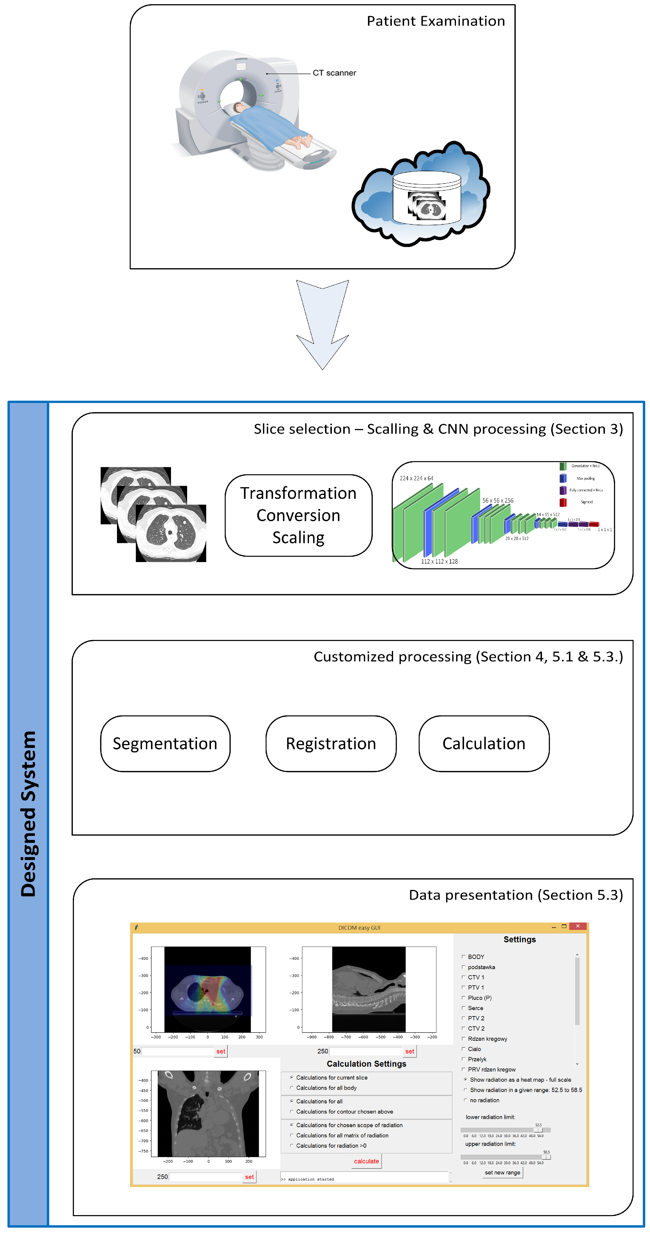
Figure 1. The general dataflow of the proposed system.
Applsci 11 01582 g001
Figure 2. The structure of the VGG network used in our system.
Applsci 11 01582 g002
Figure 3. CNN selection procedure. HU, Hounsfield unit.
Applsci 11 01582 g003
Figure 4. Example of images classified as false negative by all tested networks.
Applsci 11 01582 g004
Figure 5. Example of images classified as false positive by all tested networks.
Applsci 11 01582 g005
Figure 6. Lung segmentation results.
Applsci 11 01582 g006
Figure 7. First steps of segmentation.
Applsci 11 01582 g007
Figure 8. First steps of segmentation with trachea.
Applsci 11 01582 g008
Figure 9. Minimum y values of trachea and one lung.
Applsci 11 01582 g009
Figure 10. Distances between centroids calculations.
Applsci 11 01582 g010
Figure 11. Sobel filter application in the watershed algorithm.
Applsci 11 01582 g011
Figure 12. Example of segmented lungs.
Applsci 11 01582 g012
Figure 13. Example of the segmentation steps using the SimpleITK library.
Applsci 11 01582 g013
Figure 14. Segmented lungs in Slice No. 66 (end of the series).
Applsci 11 01582 g014
Figure 15. Illustration of the size difference in before and after slices.
Applsci 11 01582 g015
Figure 16. Illustration of the registration results using the SimpleITK library.
Applsci 11 01582 g016
Figure 17. Illustration of the affine 3D registration with raw input slices.
Applsci 11 01582 g017
Figure 18. Illustration of the affine 3D registration with segmented input slices.
Applsci 11 01582 g018
Figure 19. Illustration of the elastic registration using the SimpleITK library.
Applsci 11 01582 g019
Figure 20. Illustration of the elastic registration using the SimpleElastix library.
Applsci 11 01582 g020
Figure 21. The main window of the system.
Applsci 11 01582 g021
Figure 22. The result window with the calculation results.
Applsci 11 01582 g022
Figure 23. The possible visualization of the CT slices.
Applsci 11 01582 g023
Figure 24. CT images before and after radical radiotherapy (RT) of left lung cancer.
Applsci 11 01582 g024
Figure 25. CT images before and after radical RT of left lung cancer.
Applsci 11 01582 g025
Table 1. Hounsfield scale.
MatterHounsfield Scale Range
Bone+400 → +1000
Soft tissue+40 → +80
Water0
Fat−60 → −100
Lung−400 → −600
Air−1000
Table 2. Number of CT slices used as the input data for the CNN.
Number of CT Slices
Not LungsLungsTotal
Training data2409
(50 patients)
3293
(45 patients)
5702
Validation data567
(10 patients)
887
(12 patients)
1454
Testing data655
(13 patients)
946
(13 patients)
1601
Table 3. Confusion matrices for the validation set.
Notation
Real: LungFalse negative (FN)True positive (TP)
Real: Not lungTrue negative (TN)False positive (FP)
Predicted: Not lungPredicted: Lung
VGG16-2000
Real: Lung23864
Real: Not lung5589
Predicted: Not lungPredicted: Lung
VGG16-2500
Real: Lung11876
Real: Not lung54423
Predicted: Not lungPredicted: Lung
VGG19-2000
Real: Lung27860
Real: Not lung55512
Predicted: Not lungPredicted: Lung
VGG19-2500
Real: Lung25862
Real: Not lung55413
Predicted: Not lungPredicted: Lung
Table 4. Accuracy, sensitivity, and specificity for the validation set.
VGG19-2000VGG19-2500VGG16-2000VGG16-2500
Accuracy = (TP + TN)/All0.97320.97390.97800.9766
Sensitivity = TP/(TP + FN)0.96960.97180.97410.9876
Specificity = TN/(TN + FP)0.97880.97710.98410.9594
Table 5. Results for VGG16-2000 applied to the testing data.
Real: Lung33913Accuracy0.9763
Real: Not lung6505Sensitivity0.9651
Predicted: Not lungPredicted: LungSpecificity0.9924
Table 6. Result of one slice affine registration using SimpleITK.
ParameterValue
Transformation“Affine”
Final metric value−0.4329
Total registration time2.5 s
Table 7. Result of 3D affine registration using SimpleITK.
Raw ImagesSegmented Images
Transformation“Affine”“Affine”
Sampler‘Random’“Regular”
Final metric value−0.72−0.201
Total registration time59.5 s157.4 s
Table 8. Result of one slice elastic registration using SimpleITK.
ParameterValue
Transformation“Bspline”
Final metric value−0.3012
Total registration time21.0 s
Table 9. Result of one slice registration using SimpleElastix.
ParameterValue
Transformation 1“Affine”
Transformation 2“Bspline”
Final metric value−0.5657
Total registration time144.9 s
Publisher’s Note: MDPI stays neutral with regard to jurisdictional claims in published maps and institutional affiliations.