Abstract
The purpose of this study is (1) to provide EEG feature complexity analysis in seizure prediction by inter-ictal and pre-ital data classification and, (2) to assess the between-subject variability of the considered features. In the past several decades, there has been a sustained interest in predicting epilepsy seizure using EEG data. Most methods classify features extracted from EEG, which they assume are characteristic of the presence of an epilepsy episode, for instance, by distinguishing a pre-ictal interval of data (which is in a given window just before the onset of a seizure) from inter-ictal (which is in preceding windows following the seizure). To evaluate the difficulty of this classification problem independently of the classification model, we investigate the complexity of an exhaustive list of 88 features using various complexity metrics, i.e., the Fisher discriminant ratio, the volume of overlap, and the individual feature efficiency. Complexity measurements on real and synthetic data testbeds reveal that that seizure prediction by pre-ictal/inter-ictal feature distinction is a problem of significant complexity. It shows that several features are clearly useful, without decidedly identifying an optimal set.
1. Introduction
Epilepsy is a chronic disorder of unprovoked recurrent seizures. It affects approximately 50 million people of all ages, which makes it the second most common neurological disease [1]. Episodes of epilepsy seizure can have a significant psychological effect on patients. In addition, sudden death, called sudden unexpected death in epilepsy, can occur during or following a seizure, although this is uncommon (about 1 in 1000 patients) [2,3]. Therefore, early seizure prediction is crucial. Several studies have shown that the onset of a seizure generally follows a characteristic pre-ictal period, where the EEG pattern is different from the patterns of the seizure and also of periods preceding, called inter-ictal (Figure 1). Therefore, being able to distinguish pre-ictal and inter-ictal data patterns affords a way to predict a seizure. This can be done according to a standard pattern classification paradigm [4,5]: represent the sensed data by characteristic measurements, called features, and determine to which pattern class, pre-ictal or inter-ictal in this instance, an observed measurement belongs to. Research in seizure computer prediction has mainly followed this vein of thought. Although signal processing paradigms, such as time-series discontinuity detection, are conceivable, feature-based pattern classification is a well understood and effective framework to study seizure prediction.
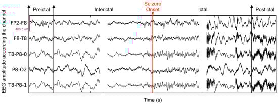
Figure 1.
The seizure phases in 5 EEG channels, including interictal, pre-ictal, ictal, and post-ictal.
To be successful, a feature-based pattern classification scheme must use efficient features, which are features that well separate the classes of patterns in the problem. Features are generally chosen following practice, as well as basic analysis and processing. The traditional paradigm of pattern recognition [4,5] uses a set of pattern-descriptive features to drive a particular classifier. The performance of the classifier-and-features combination is then evaluated on some pertinent test data. The purpose of the evaluation is not to study the discriminant potency of the features independently of the classifier, although such a study is essential to inform on the features complexity, i.e., the features classifier-independent discriminant potency. In contrast, our study is concerned explicitly with classifier-independent relative effectiveness of features. The purpose is to provide a feature complexity analysis in seizure prediction by inter-ictal/pre-ital data classification, which evaluates features using classifier-independent and statistically validated complexity metrics, such as Fisher discriminant ratio and class overlap volume, to gain some understanding of the features relative potency to inform on the complexity of epilepsy seizure prediction and the level of classification performance one can expect. This can also inform on between-patients data variability and its potential impact on epileptic seizure prediction as a pattern classifier problem. Before presenting this analysis in detail, we briefly review methods that have addressed EEG feature-based epileptic seizure prediction.
The statistical study in Reference [6] compared 30 features in terms of their ability to distinguish between the pre-ictal and pre-seizure periods, concluding that only a few features of synchronization showed discriminant potency. The method had the merit of not basing its analysis on a particular classifier. Rather, it measured a feature in pre-ictal and inter-ictal segments and evaluated the difference by statistical indicators, such as the ROC curve. This difference is subsequently mapped onto the ability of the feature to separate pre-ictal from inter-ictal segments. In general, however, epilepsy seizure prediction methods, such as References [7,8], are classifier-based because they measure a feature classification potency by its performance using a particular classification algorithm. Although a justification to use the algorithm is generally given, albeit informally, feature potency interpretation can change if a different classifier is used. Observed feature interpretation discrepancies can often be explained by the absence of statistical validation in classifier-dependent methods. The importance of statistical validation has been emphasized in Reference [9], which used recordings of 278 patients to investigate the performance of a subject-specific classifier learned using 22 features. The study reports low sensitivity and high false alarm rates compared to studies that do not use statistical validation and which, instead, report generally optimistic results. Other methods [10,11,12] have resorted to simulated pre-ictal data, referred to as surrogate data, generated by a Monte Carlo scheme, for instance, for a classifier-independent means of evaluating a classifier running on a set of given features: If its performance is better on the training data than on the surrogate data, the method is taken to be sound, or is worthy of further investigation. However, no general conclusions are drawn regarding the investigated algorithm seizure prediction ability. The study of Reference [13] investigated a patient-specific monitoring system trained from long-term EEG records, and in which seizure prediction combines decision trees and nearest-neighbors classification. Along this vein, Reference [14] used a support vector machine to classify patient-dependent, hand-crafted features. Experiments reported indicate the method decisions have high sensitivity and false alarm rates. Deep learning networks have also served seizure prediction, and studies mention that they can achieve a good compromise between sensitivity and false alarm rates [15,16].
None of the studies we have reviewed inquired into EEG feature classification complexity, in spite of the importance of this inquiry. As we have indicated earlier, a study of feature classification complexity is essential because it can inform on important properties of the data representation features, such as their mutual discriminant capability and extent, and their relative discriminant efficiency. This, in turn, can benefit feature selection and classifier design. Complexity is generally mentioned by clinicians, who acknowledge, often informally, that common subject-specific EEG features can be highly variable, and that cross-subject features are generally significantly more so. This explains in part why research has so far concentrated on subject-specific data features analysis, rather than cross-subject. Complexity analysis has the added advantage of applying equally to both subject-specific and cross-subject features, thus offering an opportunity to draw beforehand some insight on cross-subject data.
The purpose of this study was to investigate the complexity of pre-ictal and inter-ictal classification using features extracted from EEG records, to explore the predictive potential of cross-subject classifiers for epileptic seizure prediction, and evaluate the between-subject variability of the considered features. Using complexity metrics which correlate linearly to classification error [17,18,19,20], this study provides an algorithm-independent cross-subject classification complexity analysis of a set of 88 prevailing features, collected from EEG data of 24 patients. We employed such complexity measures for two-class problems to examine the individual feature ability to distinguish the inter-ictal and pre-ictal periods and to inspect the difficulty of the classification problem. The same complexity metrics generalized to multiple classes are also utilized in order to highlight the variability between patients considering the extracted features.
The remainder of this paper gives the details of the data, its processing, and analysis. It is organized as follows: Section 2 describes the materials and methods: the database, the features, the complexity metrics, and the statistical analysis. Section 3 presents experimental results, and Section 4 concludes the paper.
2. Materials and Methods
2.1. Database
We performed the complexity analysis on the openly available database collected at the Children’s Hospital Boston [21] which contains intracranial EEG records from 24 monitored patients. The EEG raws sampled at 256 Hz were filtered using notch and band-pass filters to remove some degree of artifacts and focus on relevant brain activity. Subsequently, we segmented the data to 5-s non-overlapping windows, allowing capturing relevant patterns and satisfying the condition of stationarity [22,23,24]. We set the pre-ictal period to be 30 min before the onset of the seizure as suggested in References [9,25], and eliminated 30 min after the beginning of the seizure to exclude effects from the post-ictal period, inducing a total of almost 828 remaining hours divided into 529,415 samples for the inter-ictal state and 66,782 for the pre-ictal interval.
2.2. Extracted Features
We queried relevant papers and reviews [7,26,27] which addressed epileptic seizure prediction, to collect a superset of 88 features, univariate, as well as bivariate, commonly used in epilepsy prediction. We focused on algorithm-based seizure prediction studies. Only studies which used features from EEG records were included in the study. Image-based representation studies, for instance, were excluded.
We extracted a total of 21 univariate linear features, including statistical measures, such as variance, , skewness, , and kurtosis, , temporal features, such as Hjorth parameters, HM (mobility), and HC (complexity) [28], the de-correlation time, , and the prediction error of auto-regressive modeling, , as well as spectral attributes, for instance, the spectral band power of the delta, , theta, , alpha, , beta, , and gamma, , bands, the spectral edge frequency, , the wavelet energy, , entropy, , signal energy, E, and accumulated energy, . Eleven additional univariate non-linear features from the theory of dynamical systems [29,30,31] have been used, characterizing the behavior of complex dynamical system, such the brain by using observable data (EEG records) [32,33]. Time-delay embedding reconstruction of the state space trajectory from the raw data was used to calculate the non-linear features [34]. The time delay, , and the embedding dimension, m, were chosen according to previous studies [33,35]. Within this framework, we determine the correlation dimension, [36], and correlation density, [37]. We used also the largest Lyapunov exponent, [33], and the local flow, , to assess determinism, the algorithmic complexity, , and the loss of recurrence, , to evaluate non-stationarity and, finally, the marginal predictability, [38]. Moreover, we used a surrogate-corrected version of the correlation dimension, , largest Lyapunov exponent, , local flow, , and algorithmic complexity, . We investigated also 48 linear bivariate attributes, including 45 bivariate spectral power features, [24], cross-correlation, , linear coherence, , and mutual information, . As for bivariate non-linear measures, we used 6 different characteristics for phase synchronization: the mean phase coherence, R, and the indexes based on conditional probability, , and Shanon entropy, , evaluated on both the Hilbert and wavelet transforms. Finally, we also retained two measures of non-linear interdependence, S and H.
2.3. Complexity Metrics for Pre-Ictal and Inter-Ictal Feature Classification
Data complexity analysis often has the goal to get some insight into the level of discrimination performance that can be achieved by classifiers taking into consideration intrinsic difficulties in the data. Ref. [19] observed that the difficulty of a classification problem arises from the presence of different sources of complexity: (1) the class ambiguity which describes the issue of non-distinguishable classes due to an intrinsic ambiguity or insufficient discriminant features [39], (2) the sample sparsity and feature space dimensionality expressing the impact of the number and representativeness of training set on the model’s generalization capacity [18], and (3) the boundary complexity defined by the Kolmogorov complexity [40,41] of the class decision boundary minimizing the Bayes error. Since the Kolmogorov complexity measuring the length of the shortest program describing the class boundary is claimed to be uncountable [42], various geometrical complexity measures have been deployed to outline the decision region [43]. Among the several types of complexity measures, the geometrical complexity is the most explored and used for complexity assessment [44,45,46]. Thus, for each individual extracted feature, we evaluate the geometrical complexity measures of overlaps in feature values from different classes, inspecting the efficiency of a single feature to distinguish between the inter-ictal and the pre-ictal states. We considered the following feature complexity metrics:
- Fisher discriminant ratio, F1: quantifying the separability capability between the classes. It is given by:where , , and , are the means and variances of the attribute i for each of the two classes: inter-ictal and pre-ictal, respectively. The larger the value of F1 is, the wider the margin between classes and smaller variance within classes are, such that a high value presents a low complexity problem.
- Volume of overlap region, F2: measuring the width of the entire interval encompassing the two classes. It is denoted by:where , , , are the maximums and minimums values of the feature i for the two classes, respectively. F2 is zero if the two classes are disjoint. A low value of F2 would correspond to small amount of the overlap among the classes indicating a simple classification problem.
- Individual feature efficiency, F3: describing how much an attribute contribute to distinguish between the two classes. It is defined by:where , , , are the maximums and minimums of the attribute i for each of the two classes, respectively, and n is the total number of samples in both classes. A high value of F3 refer to a good separability between the classes.
2.4. Complexity Metrics for Cross-Subject Variability Assessement
Alternatively, we resorted to the extension of complexity measures designed for a binary problem to multiple-class classification in order to study the variability of the features of the pre-ictal state between patients where the classification task is to identify to which patient a pre-ictal instance belongs. The complexity of the patient’s classification problem points out to the level of variability within patients. By converting the multi-class problem to many two-class sub-problems. The complexity metrics become:
- The Fisher discriminant ratio, F1, for C classes extended from Equation (1) as:where , , , , and are the means, the proportions, and the variance of the feature i for the two classes j and k, respectively.
- The volume of overlap region, F2, for a multi-class problem is given by:where , , , are the maximums and minimums values of the feature i for the two classes j and k, respectively.
- The individual feature efficiency for multiple classes can be written as:where , , , are the maximums and minimums of the attribute i for the classes i and j, respectively, and is the total number of samples.
Furthermore, for each complexity measure evaluated for all 88 extracted features, we estimate the data distribution by fitting the data with 82 distribution functions available in the SciPy 0.12.0 Package. To test the goodness of fit, we perform a Kolmogorov-Smirnov test, with a significance level of 0.05. Lower and upper thresholds, on which the decision whether the feature is complex or not relies, are set according to the rule of thumbs to the 5th and 95th quantiles of the probability distribution which fits the best the data. The feature that exceeds the lower or higher threshold, depending on the complexity metric, is considered a potential discriminant feature.
2.5. Statistical Analysis
Following the complexity metrics assessment, we conduct a statistical test to certify that the analysis results are significant. We performed the t-test for each retained feature, distinguishing the inter-ictal and pre-ictal classes, to assess how significant the difference between the categories. For the between-patient variability study, since classifying the pre-ictal samples by patients is a multi-class problem, we applied the one-way ANOVA test to verify that the promising discriminant features are significantly different between subjects. The classes are said to differ significantly if the p-value of the statistical test is smaller than a two-sided significance level of .
3. Results and Discussion
As described earlier, we conducted our experiments on the public CHB-MIT dataset described in Section 2.1. A total of 88 univariate and bivariate features commonly used in epilepsy prediction have been extracted from the EEG records (as presented in Section 2.2). The pre-processing of the dataset and the feature extraction were done using MATLAB R2020a software.
3.1. Analysis of the Complexity of the Pre-Ictal and Inter-Ictal Features
To illustrate the feature complexity analysis, three metrics are evaluated on the extensive list of the extracted features: F1, F2, and F3. The lower and higher threshold values have been identified, for each complexity metric, using a probability density which best fit each complexity data. Figure 2 illustrates the empirical and fitted distribution for each complexity measure.
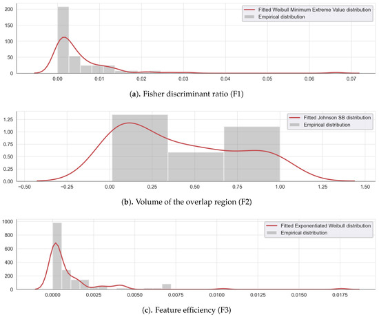
Figure 2.
Empirical and fitted distribution for the complexity measures: (a) Fisher discriminant ratio F1, (b) the volume of the overlap interval F2, and (c) the individual feature efficiency F3.
The Fisher discriminant ratio F1 can be modeled by a Weilbull minimum extreme value distribution (Figure 2a), the volume of overlap region F2, follows a Johnson SB distribution (Figure 2b) and the feature efficiency values F3, can be approximated by an exponentiated Weilbull distribution (Figure 2c). Following this modeling, the lower and upper threshold values are determined using the 5th and the 95th percentiles of each complexity measure empirical density, as shown in Table 1.

Table 1.
Thresholds for the complexity metrics.
The results of evaluating the Fisher discriminant ratio, F1, on various features, are shown in Figure 3a. The threshold was set to 0.017 (Table 1 line 1). As shown in Figure 3a, three bivariate spectral power attributes, , , and and the mutual information, , surpass the threshold value. Because higher values indicate better class separation, only these features are retained.
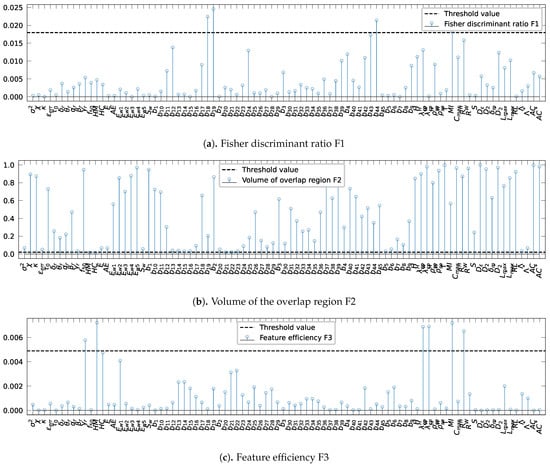
Figure 3.
Evaluation of the complexity metrics for each extracted value: (a) Fisher discriminant ratio, F1: a high value of F1 shows that the feature is discriminant, (b) the volume of the overlap interval, F2: a low value of F2 indicates small amount of overlap among the classes, and (c) the individual feature efficiency, F3: a high value of F3 implies a good separability between the classes. The horizontal dotted blue represents the threshold values.
Likewise, Figure 3b presents the results obtained by the assessment of the volume of overlap region, F2. Given the threshold 0.02 (Table 1, line 2), only the two Hjorth parameters, HM and HC, are retained since lower values indicate a small amount of overlap among the classes.
In Figure 3c, the individual feature efficiency, F3, values for each characteristic are shown. For this complexity metric, the threshold is set to 0.0048 (Table 1, line 3). The features having a higher value of F3 than the threshold value are the relative gamma band spectral power, , the Hjorth parameter, HM, the mean phase coherence using the Hilbert transform, , and the indexes measures for phase synchronization based on conditional probability, and . Thus, the features are retained because high values of F3 claim a good feature separability between the categories.
In summary, the analysis of the extracted features complexity reveals that only ten out of 88 attributes has been picked as not complex. We observed also an overlap between the different feature obtained by each complexity metrics, such as the Hjorth parameter, HM, which has a low value of volume of overlap, F2, and high value of the feature efficiency, F3. According to Table 2 summarizing the list of the retained features, all ten features have a p-value corresponding to the statistical t-test lower than the critical value for 5% significance level, which approves that the features are statistically significantly different, thus confirming their ability to discriminate between the two classes.
Table 2.
Retained attributes from the feature complexity analysis, their types, and the corresponding p-value of the t-test.
We observe that only three non-linear features, the mean phase coherence using the Hilbert transform and the two measures for phase synchronization, the indexes based on conditional probability, and , all bivariate, are retained as discriminant, declaring they are the best discriminant non-linear bivariate features and that most of the non-linear other features especially univariate characteristics are incapable to distinguish between the inter-ictal and pre-seizure times, as also observed by [6,47,48]. The Hjorth parameters, HM, and HC, are also shown to be the most uni-variate linear discriminant features of the two states as substantiated in Reference [6]. The other linear univariate recalled feature as discriminant is the relative gamma-band spectral power, , which supports the studies [23,49] saying that the characteristics from the gamma band are more relevant than other bands for the epilepsy prediction.
Despite of extracting many linear and non-linear both univariate and bivariate features from EEG records, we found that a restricted number of attributes shown to be promising to distinguish the inter-inctal and pre-ictal classes.
Comparison with reference databases: To have some insight into the complexity of the classification problem of inter-ictal and pre-ictal states, we compared our results against known relatively simple classification problems from the UC-Irvine Machine Learning Depository [50] and other randomly labeled synthetic data. We estimate the complexity measures of three binary classification problems from the Iris dataset and a linearly non-separable problem using the Letter database of 20,000 samples with 16 attributes. We also used a more complex dataset for the human activity recognition (HAR) using sensor signals (accelerometer and gyroscope) recorded from a waist-mounted smartphone. The dataset contains 10,299 samples with 561 features. Moreover, we evaluate the complexity metrics on two artificial classification problems, obtained from randomly labeling uniformly distributed data points, containing, respectively, 10,000 samples with a single feature, and 600,000 with 88 dimensions.
The results summarized in Table 3 show that the maximum Fisher discriminant ratio of the epilepsy dataset is lower than simpler problems, for instance, classification tasks from the iris and letter sets and higher than results from the random noise sets. Indeed, the maximum Fisher discriminant ratio is 0.0245 for epilepsy data, 31.19, 49.94, and 4.27 for the Versicolor-Virginica, Setosa-Virginica, and Setosa-Versicolor, respectively, from the Iris data, 0.9 for the Letter dataset, 2.66 for the human activity recognition (HAR) dataset, and 1.7 × 10 and 1.66 × 10 for the two random datasets. Similarly, the maximum feature efficiency of easy classification problems from Iris and Letter data, and for a relatively complex classification problem, such as human activity recognition, given the HAR dataset, is higher than 0.25, unlike the epilepsy data having a low value of 0.003 and the two random data having, respectively, a maximum feature efficiency of and 1.66 × 10. Hence, the maximum feature efficiency of the epilepsy prediction problem is not as high as the comparatively easy problem nor as low as the intrinsically complex random noise problem. Therefore, this shows evidence that the epilepsy data does contain learnable structures, yet the classification problem using the extracted features from the EEG records is highly complex.
Table 3.
Comparison of the maximum Fisher discriminant ratio and the maximum feature efficiency for various classification problems: (1) Iris: Versicolor-Virginica, (2) Iris: Setosa-Virginica, (3) Iris: Setosa-Versicolor, (4) Letter recognition, (5) epilepsy prediction, (6) human activity recognition (HAR) and couple random noise sets, (7) random data 1 and, (8) random data 2.
3.2. Cross-Patient Variability Assessement
To get a deeper insight into the epilepsy prediction problem formulated as a classification of inter-ictal and pre-ictal intervals using extracted features from EEG raws, it is necessary to check the variability of the information characterizing the pre-ictal state across patients. Therefore, similar to the suggested strategy to evaluate the complexity of the pre-ictal and inter-ictal classification, we analyze the data complexity measures for the extracted features from the pre-ictal state of all patients, where the classification task is to categorize the pre-ictal instances by patients, under the hypothesis that the simplicity of the classification task implies a high variability of the features between patients.
The assessment of the complexity measures: the Fisher discriminant ratio, F1, the volume of overlap region, F2, and the feature efficiency, F3, are shown in Figure 4.
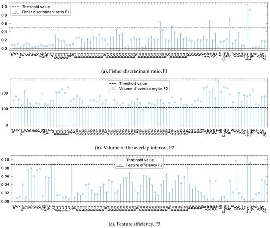
Figure 4.
Evaluation of the complexity metrics: (a) Fisher discriminant ratio, F1, (b) the volume of the overlap interval, F2, and (c) the individual feature efficiency, F3. The horizontal dotted blue indicates the threshold values.
Threshold values were defined as the 5th and 95th quantiles of the best-fitted distribution of each complexity measure data shown in Figure 5 are resumed in Table 4. For the metrics F1, and F3, the thresholds were set to 0.48 (Table 4, line 1) and 0.087 (Table 4, line 3), while, for F2, the threshold was set to 160 (Table 4, line 2).
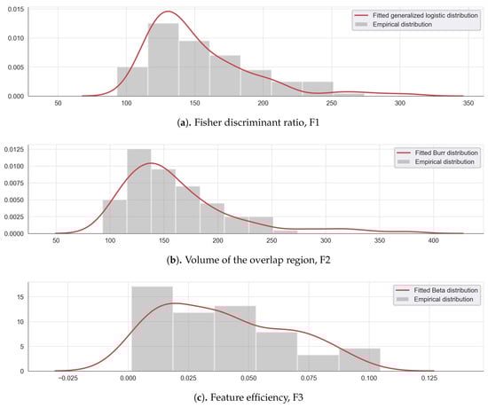
Figure 5.
Empirical and fitted distribution for the complexity measures (a) Fisher discriminant ratio F1, (b) the volume of the overlap interval F2, and (c) the individual feature efficiency F3.
Table 4.
Thresholds for the complexity metrics.
Figure 4 presents the evaluation with different complexity metrics. Figure 3a reveals that two bivariate spectral power attributes, and , the mean phase coherence, R, and the indexes based on conditional probability, , and Shanon entropy, , evaluated both using the wavelet transform, the largest Lyapunov exponent, , and the surrogate-corrected version of the largest Lyapunov exponent, , exceed the Fisher discriminant ratio threshold value of 0.48. For the volume of the overlap region interval, only four bivariate spectral power attributes, , , , and , and the correlation density, , exceed the threshold value, as shown in Figure 3b. Finally, Figure 3c displays the results of the assessment of the feature efficiency, showing that the variance, , signal energy, E, accumulated energy, , correlation density, , largest Lyapunov exponent, , and the surrogate-corrected version of the largest Lyapunov exponent, , have higher values than the threshold . In conclusion, a total of 14 out of 88 features are shown to distinguish well the pre-ictal observations by patient. Therefore, performing the one-way ANOVA test for each of the fourteen recalled features exhibits significant differences between patients as null p-values are obtained for all the features, which validates that each individual characteristic has large between-class distances. As a result, it is safe to conclude that the extracted features from the pre-ictal state vary significantly between patients, which raises a concern when using cross-patient models in real-world applications. Moreover, the high variability of the extracted features motivates research on searching new invariant features between patients.
4. Conclusions
This study investigated the complexity of a superset of EEG-based features commonly practiced to distinguish an inter-ictal period from a pre-ictal in epileptic seizure prediction. The investigation is based on a classifier-independent complexity analysis which used complexity measures, such as the Fisher discriminant ratio and the volume of class overlap in feature space, to evaluate the discriminant potency of each feature. Implemented using the publicly available Boston Children’s Hospital database of EEG records, the analysis supports the conclusion that the features and, thereof, feature-based distinction of the pre-ictal and inter-ictal periods in EEG records, are highly complex.
This study can be strengthened along three majors veins. Along one vein, larger amounts of data, using different other EEG databases, can confirm and strengthen its conclusions on feature complexity and inter-subject variability. Along a second vein, features other than those generally practiced, which are those used in this study, can be investigated. To this end, feature computation by deep machine learning is exceptionally promising, as it has had recently a remarkable performance with similar and more difficult data. Finally, it can be of significant benefit to investigate domain adaptation for EEG data, whereby the dependence on large amounts of data for accurate EEG-based decision can be alleviated.
Author Contributions
Conceptualization, I.J., A.M., and N.M.; methodology, I.J., A.M., and N.M.; software, I.J.; validation, A.M.and N.M.; formal analysis, I.J.; investigation, I.J., A.M., and N.M.; resources, N.M.; data curation, I.J.; writing—original draft preparation, I.J.; writing—review and editing, A.M. and N.M.; visualization, I.J.; supervision, A.M. and N.M.; project administration, A.M. and N.M.; funding acquisition, I.J., A.M., and N.M. All authors have read and agreed to the published version of the manuscript.
Funding
This research was supported by the Canada Research Chair on Biomedical Data Mining (950-231214) and the discovery grant (RGPIN-2020-06313).
Institutional Review Board Statement
Not applicable.
Informed Consent Statement
Not applicable.
Data Availability Statement
The CHB-MIT Scalp EEG Database is available at https://physionet.org/content/chbmit/1.0.0/ (accessed on 9 June 2020).
Acknowledgments
This research was supported by the Canada Research Chair on Biomedical Data Mining (950-231214).
Conflicts of Interest
The authors declare no conflict of interest.
Abbreviations
The extracted features from EEG records used in the complexity analysis.
| Symbols | Extracted features |
| variance | |
| skewness | |
| kurtosis | |
| HM | Hjorth parameter (mobility) |
| HC | Hjorth parameter (complexity) |
| decorrelation time | |
| error of the auto-regressive modeling | |
| relative power of the delta spectral band | |
| relative power of the theta spectral band | |
| relative power of the alpha spectral band | |
| relative power of the beta spectral band | |
| relative power of the gamma spectral band | |
| spectral edge frequency | |
| wavelet energy | |
| wavelet entropy | |
| E | signal energy |
| signal accumulated energy | |
| correlation dimension | |
| correlation density | |
| largest Lyapunov exponent | |
| local flow | |
| algorithmic complexity | |
| loss of recurrence | |
| marginal predictability | |
| surrogate-corrected version of the correlation dimension | |
| surrogate-corrected version of the largest Lyapunov exponent | |
| surrogate-corrected version of the local flow | |
| surrogate-corrected version of the algorithmic complexity | |
| bivariate spectral power features | |
| cross correlation | |
| linear coherence | |
| mutual information | |
| R | mean phase coherence |
| index based on conditional probability using the wavelet transform | |
| index based on conditional probability using the Hilbert transform | |
| index based on Shannon entropy using the wavelet transform | |
| index based on Shannon entropy using the Hilbert transform | |
| S | non-linear interdependence measure |
| H | non-linear interdependence normalized measure |
References
- World Health Organization. Epilepsy; World Health Organization: Geneva, Switzerland, 2019. [Google Scholar]
- Coll, M.; Allegue, C.; Partemi, S.; Mates, J.; Del Olmo, B.; Campuzano, O.; Pascali, V.; Iglesias, A.; Striano, P.; Oliva, A.; et al. Genetic investigation of sudden unexpected death in epilepsy cohort by panel target resequencing. Int. J. Leg. Med. 2016, 130, 331–339. [Google Scholar] [CrossRef] [PubMed]
- Partemi, S.; Vidal, M.C.; Striano, P.; Campuzano, O.; Allegue, C.; Pezzella, M.; Elia, M.; Parisi, P.; Belcastro, V.; Casellato, S.; et al. Genetic and forensic implications in epilepsy and cardiac arrhythmias: A case series. Int. J. Leg. Med. 2015, 129, 495–504. [Google Scholar] [CrossRef]
- Duda, R.O.; Hart, P.E.; Stork, D.G. Pattern Classification; John Wiley & Sons: New York, NY, USA, 2012. [Google Scholar]
- Bishop, C.M. Pattern Recognition and Machine Learning; Springer: New York, NY, USA, 2006. [Google Scholar]
- Mormann, F.; Kreuz, T.; Rieke, C.; Andrzejak, R.; Kraskov, A.; David, P.; Elger, C.; Lehnertz, K. On the predictability of epileptic seizures. Clin. Neurophysiol. Off. J. Int. Fed. Clin. Neurophysiol. 2005, 116, 569–587. [Google Scholar] [CrossRef]
- Assi, E.B.; Nguyen, D.K.; Rihana, S.; Sawan, M. Towards accurate prediction of epileptic seizures: A review. Biomed. Signal Process. Control. 2017, 34, 144–157. [Google Scholar] [CrossRef]
- Gadhoumi, K.; Lina, J.M.; Mormann, F.; Gotman, J. Seizure prediction for therapeutic devices: A review. J. Neurosci. Methods 2016, 260, 270–282. [Google Scholar] [CrossRef]
- Teixeira, C.A.; Direito, B.; Bandarabadi, M.; Le Van Quyen, M.; Valderrama, M.; Schelter, B.; Schulze-Bonhage, A.; Navarro, V.; Sales, F.; Dourado, A. Epileptic seizure predictors based on computational intelligence techniques: A comparative study with 278 patients. Comput. Methods Programs Biomed. 2014, 114, 324–336. [Google Scholar] [CrossRef] [PubMed]
- Andrzejak, R.G.; Mormann, F.; Kreuz, T.; Rieke, C.; Kraskov, A.; Elger, C.E.; Lehnertz, K. Testing the null hypothesis of the nonexistence of a preseizure state. Phys. Rev. E 2003, 67, 010901. [Google Scholar] [CrossRef]
- Andrzejak, R.G.; Chicharro, D.; Elger, C.E.; Mormann, F. Seizure prediction: Any better than chance? Clin. Neurophysiol. 2009, 120, 1465–1478. [Google Scholar] [CrossRef] [PubMed]
- Kreuz, T.; Andrzejak, R.G.; Mormann, F.; Kraskov, A.; Stögbauer, H.; Elger, C.E.; Lehnertz, K.; Grassberger, P. Measure profile surrogates: A method to validate the performance of epileptic seizure prediction algorithms. Phys. Rev. E 2004, 69, 061915. [Google Scholar] [CrossRef] [PubMed]
- Cook, M.J.; O’Brien, T.J.; Berkovic, S.F.; Murphy, M.; Morokoff, A.; Fabinyi, G.; D’Souza, W.; Yerra, R.; Archer, J.; Litewka, L.; et al. Prediction of seizure likelihood with a long-term, implanted seizure advisory system in patients with drug-resistant epilepsy: A first-in-man study. Lancet Neurol. 2013, 12, 563–571. [Google Scholar] [CrossRef]
- Moghim, N.; Corne, D.W. Predicting epileptic seizures in advance. PLoS ONE 2014, 9, e99334. [Google Scholar] [CrossRef] [PubMed]
- Tsiouris, K.M.; Pezoulas, V.C.; Zervakis, M.; Konitsiotis, S.; Koutsouris, D.D.; Fotiadis, D.I. A long short-term memory deep learning network for the prediction of epileptic seizures using EEG signals. Comput. Biol. Med. 2018, 99, 24–37. [Google Scholar] [CrossRef] [PubMed]
- Daoud, H.; Bayoumi, M.A. Efficient epileptic seizure prediction based on deep learning. IEEE Trans. Biomed. Circuits Syst. 2019, 13, 804–813. [Google Scholar] [CrossRef] [PubMed]
- Ho, T.K. A data complexity analysis of comparative advantages of decision forest constructors. Pattern Anal. Appl. 2002, 5, 102–112. [Google Scholar] [CrossRef]
- Bernadó-Mansilla, E.; Ho, T.K. Domain of competence of XCS classifier system in complexity measurement space. IEEE Trans. Evol. Comput. 2005, 9, 82–104. [Google Scholar] [CrossRef]
- Ho, T.K.; Bernadó-Mansilla, E. Classifier domains of competence in data complexity space. In Data Complexity in Pattern Recognition; Springer: London, UK, 2006; pp. 135–152. [Google Scholar]
- Mansilla, E.B.; Ho, T.K. On classifier domains of competence. In Proceedings of the 17th IEEE International Conference on Pattern Recognition, ICPR 2004, Cambridge, UK, 26 August 2004; Volume 1, pp. 136–139. [Google Scholar]
- Shoeb, A.H. Application of Machine Learning to Epileptic Seizure Onset Detection and Treatment. Ph.D. Thesis, Massachusetts Institute of Technology, Cambridge, MA, USA, 2009. [Google Scholar]
- Rasekhi, J.; Mollaei, M.R.K.; Bandarabadi, M.; Teixeira, C.A.; Dourado, A. Preprocessing effects of 22 linear univariate features on the performance of seizure prediction methods. J. Neurosci. Methods 2013, 217, 9–16. [Google Scholar] [CrossRef] [PubMed]
- Assi, E.B.; Sawan, M.; Nguyen, D.; Rihana, S. A hybrid mRMR-genetic based selection method for the prediction of epileptic seizures. In Proceedings of the 2015 IEEE Biomedical Circuits and Systems Conference (BioCAS), Atlanta, GA, USA, 22–24 October 2015; pp. 1–4. [Google Scholar]
- Bandarabadi, M.; Teixeira, C.A.; Rasekhi, J.; Dourado, A. Epileptic seizure prediction using relative spectral power features. Clin. Neurophysiol. 2015, 126, 237–248. [Google Scholar] [CrossRef] [PubMed]
- Bandarabadi, M.; Rasekhi, J.; Teixeira, C.A.; Karami, M.R.; Dourado, A. On the proper selection of preictal period for seizure prediction. Epilepsy Behav. 2015, 46, 158–166. [Google Scholar] [CrossRef]
- Mormann, F.; Andrzejak, R.G.; Elger, C.E.; Lehnertz, K. Seizure prediction: The long and winding road. Brain 2007, 130, 314–333. [Google Scholar] [CrossRef] [PubMed]
- Teixeira, C.; Direito, B.; Feldwisch-Drentrup, H.; Valderrama, M.; Costa, R.; Alvarado-Rojas, C.; Nikolopoulos, S.; Le Van Quyen, M.; Timmer, J.; Schelter, B.; et al. EPILAB: A software package for studies on the prediction of epileptic seizures. J. Neurosci. Methods 2011, 200, 257–271. [Google Scholar] [CrossRef] [PubMed]
- Damaševičius, R.; Maskeliūnas, R.; Woźniak, M.; Połap, D. Visualization of physiologic signals based on Hjorth parameters and Gramian Angular Fields. In Proceedings of the 2018 IEEE 16th World Symposium on Applied Machine Intelligence and Informatics (SAMI), Kosice, Slovakia, 7–10 February 2018; pp. 000091–000096. [Google Scholar]
- Schuster, H.G.; Just, W. Deterministic Chaos: An Introduction; John Wiley & Sons: Hoboken, NJ, USA, 2006. [Google Scholar]
- Ott, E. Chaos in Dynamical Systems; Cambridge University Press: Cambridge, UK, 2002. [Google Scholar]
- Kantz, H.; Schreiber, T. Nonlinear Time Series Analysis; Cambridge University Press: Cambridge, UK, 2004; Volume 7. [Google Scholar]
- Andrzejak, R.G.; Widman, G.; Lehnertz, K.; Rieke, C.; David, P.; Elger, C. The epileptic process as nonlinear deterministic dynamics in a stochastic environment: An evaluation on mesial temporal lobe epilepsy. Epilepsy Res. 2001, 44, 129–140. [Google Scholar] [CrossRef]
- Iasemidis, L.D.; Sackellares, J.C.; Zaveri, H.P.; Williams, W.J. Phase space topography and the Lyapunov exponent of electrocorticograms in partial seizures. Brain Topogr. 1990, 2, 187–201. [Google Scholar] [CrossRef] [PubMed]
- Damasevicius, R.; Martisius, I.; Jusas, V.; Birvinskas, D. Fractional delay time embedding of EEG signals into high dimensional phase space. Elektron. Elektrotechnika 2014, 20, 55–58. [Google Scholar] [CrossRef]
- Iasemidis, L.; Principe, J.; Sackellares, J. Measurement and quantification of spatiotemporal dynamics of human epileptic seizures. Nonlinear Biomed. Signal Process. 2000, 2, 294–318. [Google Scholar]
- Lehnertz, K.; Andrzejak, R.G.; Arnhold, J.; Kreuz, T.; Mormann, F.; Rieke, C.; Widman, G.; Elger, C.E. Nonlinear EEG Analysis in Epilepsy: Its Possible Use for Interictal Focus Localization, Seizure Anticipation, and. J. Clin. Neurophysiol. 2001, 18, 209–222. [Google Scholar] [CrossRef] [PubMed]
- Lerner, D.E. Monitoring changing dynamics with correlation integrals: Case study of an epileptic seizure. Phys.-Sect. D 1996, 97, 563–576. [Google Scholar] [CrossRef]
- Savit, R.; Green, M. Time series and dependent variables. Phys. D Nonlinear Phenom. 1991, 50, 95–116. [Google Scholar] [CrossRef]
- Ho, T.K.; Baird, H.S. Large-scale simulation studies in image pattern recognition. IEEE Trans. Pattern Anal. Mach. Intell. 1997, 19, 1067–1079. [Google Scholar]
- Kolmogorov, A.N. Three approaches to the quantitative definition ofinformation. Probl. Inf. Transm. 1965, 1, 1–7. [Google Scholar]
- Li, M.; Vitányi, P. An Introduction to Kolmogorov Complexity and Its Applications; Springer: New York, NY, USA, 2008; Volume 3. [Google Scholar]
- Maciejowski, J.M. Model discrimination using an algorithmic information criterion. Automatica 1979, 15, 579–593. [Google Scholar] [CrossRef]
- Basu, M.; Ho, T.K. Data Complexity in Pattern Recognition; Springer Science & Business Media: London, UK, 2006. [Google Scholar]
- Mezghani, N.; Mechmeche, I.; Mitiche, A.; Ouakrim, Y.; De Guise, J.A. An analysis of 3D knee kinematic data complexity in knee osteoarthritis and asymptomatic controls. PLoS ONE 2018, 13, e0202348. [Google Scholar] [CrossRef] [PubMed]
- Morán-Fernández, L.; Bolón-Canedo, V.; Alonso-Betanzos, A. Centralized vs. distributed feature selection methods based on data complexity measures. Knowl.-Based Syst. 2017, 117, 27–45. [Google Scholar] [CrossRef]
- Sun, M.; Liu, K.; Wu, Q.; Hong, Q.; Wang, B.; Zhang, H. A novel ECOC algorithm for multiclass microarray data classification based on data complexity analysis. Pattern Recognit. 2019, 90, 346–362. [Google Scholar] [CrossRef]
- Harrison, M.A.F.; Osorio, I.; Frei, M.G.; Asuri, S.; Lai, Y.C. Correlation dimension and integral do not predict epileptic seizures. Chaos Interdiscip. J. Nonlinear Sci. 2005, 15, 033106. [Google Scholar] [CrossRef] [PubMed]
- McSharry, P.E.; Smith, L.A.; Tarassenko, L. Prediction of epileptic seizures: Are nonlinear methods relevant? Nat. Med. 2003, 9, 241–242. [Google Scholar] [CrossRef] [PubMed]
- Park, Y.; Luo, L.; Parhi, K.K.; Netoff, T. Seizure prediction with spectral power of EEG using cost-sensitive support vector machines. Epilepsia 2011, 52, 1761–1770. [Google Scholar] [CrossRef] [PubMed]
- Dua, D.; Graff, C. UCI Machine Learning Repository; University of California, School of Information and Computer Science: Irvine, CA, USA, 2017. [Google Scholar]


Publisher’s Note: MDPI stays neutral with regard to jurisdictional claims in published maps and institutional affiliations. |
© 2021 by the authors. Licensee MDPI, Basel, Switzerland. This article is an open access article distributed under the terms and conditions of the Creative Commons Attribution (CC BY) license (http://creativecommons.org/licenses/by/4.0/).