Abstract
The synchronization and control of chaos have been under extensive study by researchers in recent years. In this study, an adaptive Takagi–Sugeno–Kang (TSK) fuzzy self-organizing recurrent cerebellar model articulation controller (ATFSORC) is proposed, which is composed of a set of TSK fuzzy rules, a cerebellar model articulation controller (CMAC), a recurrent CMAC (RCMAC), a self-organizing CMAC (SOCMAC), and a compensation controller. Specifically, SOCMAC, RCMAC, and adaptive laws are adopted so that the association memory layers of ATFSORC can be modulated in accordance with the layer decision-making mechanism in order to reduce the structure complexity and improve the control performance of ATFSORC. Moreover, the Takagi–Sugeno–Kang fuzzy rules are introduced to increase the learning speed of ATFSORC, and the improved compensating controller is designed to dispel the errors between an ideal controller and the TFSORC. Moreover, the proposed ATFSORC is applied to chaotic systems in order to validate its performance and feasibility. Several simulation schemes are demonstrated to show the effectiveness of the proposed method. Simulation results show that the proposed ATFSORC can obtain a favorable control performance when the chaotic systems are operated at different parameters. Specifically, ATFSORC can achieve faster convergence of the tracking error than fuzzy CMAC (FCMAC) and CMAC.
1. Introduction
Chaos is ubiquitous and exists in various scientific fields. Therefore, it has been receiving attention widely from many scholars and has been extensively studied [1,2,3,4,5]. The chaotic system is very sensitive to the initial conditions, so the behavior of a chaotic system is eventually unpredictable. If the chaotic phenomenon can be appropriately controlled, it may be of tremendous benefit in various applications because of the highly nonlinear characteristics of chaotic systems. The research overview for the synchronization and stability control of chaotic systems is discussed below.
Tao et al. proposed a type of synchronization control between gap junction-coupled neurons [6]. They used the advantage of the chattering-free feature in the adaptive sliding mode to perform chaotic synchronization. Hsu proposed a chaotic synchronization system based on a Takagi–Sugeno–Kang (TSK)-type Hermite neural network [7]. The control system consists of an artificial neural controller and a compensator, which provide good control performance. Lin et al. proposed a recurrent fuzzy cerebellar model articulation controller and used signed distance to convert dual input variables into single input variables, thereby reducing controller architectural complexity [8]. Che et al. proposed a robust adaptive artificial neural network controller for the synchronization of two synchronous gap junction-coupled neurons in order to synchronize the chaotic system by appropriately selecting the control parameters [9]. Wu et al. proposed an adaptive TSK cerebellar model articulation controller for chaotic master–slave system synchronization by using TSK fuzzy rules and demonstrated good control tracking performance [10]. Wen et al. proposed a recurrent fuzzy cerebellar model articulation controller for dual-axis piezoelectric actuators with an input space quantization method and self-tuning learning rates [11]. This method allows the traditional cerebellar model articulation controller to have dynamic characteristics and ameliorate the shortcomings of a traditional cerebellar model, and it is effectively applied on uncertain systems. Lin et al. proposed a TSK fuzzy cerebellar model articulation controller for uncertain nonlinear systems as a tracking controller, in which the control system contains a TSK fuzzy cerebellar model articulation controller and a robust compensation controller; even if the system model is unknown, it can still achieve good tracking performance [12]. Lian et al. proposed an adaptive fuzzy self-organizing sliding-mode controller for active suspension systems by adding a sliding surface, and the stability could be more easily proven than by the traditional self-organizing fuzzy controller. Its model-free control design possesses online learning ability, which can be applied on any interfering complex system [13]. Lin et al. proposed a novel self-organizing wavelet cerebellar model articulation controller, which is applied on a nonlinear chaotic system [14]. By structure learning, it can correct the number of memory layers in real time to achieve the optimal wavelet cerebellar model articulation controller architecture, and by parameter learning, it can adjust the weight of the wavelet cerebellar model articulation controller to achieve the optimal approximation performance, and thus achieve a better control response. Chen proposed an architecture based on the TSK-type self-organizing recurrent artificial neural network that can generate or eliminate through self-organizing in order to obtain a network structure of an appropriate size [15]. Che et al. proposed an adaptive sliding-mode neural network and used a radial basis function to implement two gap junction-coupled neuron models for achieving chaotic synchronization [16].
In recent years, with the unceasing update and breakthrough of higher control theory, many outstanding scholars in the control field have successively proposed advanced control theories, such as the fuzzy control, artificial neural network (ANN), wavelet neural network (WNN), and self-organizing fuzzy control for nonlinear chaotic systems, switched-reluctance motor drive systems, voice coil motors, and permanent magnet synchronous motors. All have a fairly high reference value. Peng et al. proposed an adaptive recurrent cerebellar model articulation controller for linear ultrasonic motors, which facilitated dynamic performance and faster learning speed for the traditional cerebellar model articulation controller; they used the method of steepest descent to update the dynamic parameters of the controller in real time, thereby achieving the optimal learning velocity such that the tracking error is quickly converged [17]. Hung et al. proposed a wavelet fuzzy neural network that adopts an asymmetric membership function to ameliorate differential evolution algorithms, which are used to control an electric power steering system of a six-phase permanent magnet synchronous motor; it combines the advantages of the wavelet decomposition, fuzzy logic system, and asymmetric membership function [18]. It was developed to realize the control performance and stability required in electric power steering systems. Lin et al. proposed a novel adaptive wavelet fuzzy cerebellar model articulation control system for trajectory tracking control of voice coil motors; this control system includes a wavelet fuzzy cerebellar model articulation controller and a fuzzy compensation controller [19]. Since the wavelet function possessing differential characteristics and fuzzy are adopted, the controller has fast learning ability, due to which it shows significant performance and good tracking characteristics. Li et al. proposed a sliding-mode control method to be applied on a permanent magnet synchronous motor and added an interference estimator for feed-forward compensation; therefore, the controller possesses good robustness and can use a lower switching gain to ameliorate the chattering phenomenon of the sliding mode [20]. Lin et al. proposed a dynamic Petri-fuzzy cerebellar model articulation controller, which was applied on a magnetic levitation system and a piezoelectric motor drive system; by adding the Petri network, the burden of parameter learning is reduced [20]. Lin et al. proposed a recurrent neural network based on differential algorithms and applied it to squirrel-cage induction generators, which can process nonlinear and non-differentiable functions through differential algorithms [20]. Lin et al. proposed a type of function-linked neural network using an asymmetric radial basis function for the three-dimensional motion control of a piezoelectric platform; by using an asymmetric radial basis function, the learning ability of the network can be improved [21]. Lin et al. proposed a type of TSK neural network controller using an asymmetric radial basis function; they used the architecture of functional fuzzy rules to improve the learning rate and applied it to a three-phase grid-connected photovoltaic system [22].
The aim of this research is to develop an adaptive TSK fuzzy self-organizing recurrent cerebellar model articulation controller (ATFSORC) for the synchronization and stability control of chaotic systems. By using ATFSORC, the master and slave systems that are seemingly in a chaotic state can be adjusted according to the reciprocal errors so that the slave system can be synchronized with the master system under different initial conditions. Moreover, TSK fuzzy rules are introduced into a recurrent cerebellar model articulation controller (RCMAC), which is combined with a self-organizing CMAC (SOCMAC) and an improved compensation controller to design the ATFSORC. By adopting the architecture combining SOCMAC, RCMAC, and adaptive laws, the cerebellar model articulation controller can possess dynamic memory performance and layer correction capability. Specifically, in the proposed controller, the number of association memory layers is modulated in accordance with the layer decision-making mechanism to reduce the architectural complexity of the ATFSORC and improve the control performance. The ATFSORC controller takes integrated error function as the input, which is then introduced into the TSK fuzzy self-organizing recurrent cerebellar model articulation controller, and an improved compensation controller is taken to compensate the errors between the ideal controller and TSK fuzzy self-organizing recurrent cerebellar model articulation controller. Moreover, this study adopted Lyapunov theorem to deduce the adaptive laws for the cerebellar model articulation controller’s weight value, TSK fuzzy rules’ parameter, recurrent weight value, Gaussian function midpoint, and Gaussian function standard deviation in order to ensure the stability of the system. Then, the proposed ATFSORC is applied to chaotic systems in order to validate its performance and feasibility. Table 1 shows the full forms and the corresponding abbreviations used in this study for better information.

Table 1.
Full forms and the corresponding abbreviations used in this study.
2. Cerebellar Model Articulation Controller Theory
A cerebellar model articulation controller (CMAC) is a new neurological architecture proposed by Albus et al. in 1975 [23,24,25,26]. CMAC is a learning structure that mimics the human cerebellum. It is a neural network based on partial learning and can approximate nonlinear continuous functions with arbitrary precision. The CMAC neural network not only can hierarchically represent information but also can correct the partial weight coefficient. The learning velocity is high and the structure is simple. It possesses the advantages of local generalization, which makes it easier to be applied in real-time control compared with other neural networks; hence, it is one of the most widely applied neural networks in control.
As suggested by its name, the so-called cerebellar model articulation controller is derived by mimicking the operating manner of the human cerebellum. The architecture of CMAC is somewhat similar to an artificial neural network; in fact, it can be regarded as a simplified artificial neural network. The biggest difference is that unlike the artificial neural network, which uses only the triggered memory in each learning, CMAC will use all the memories in each learning, thereby drastically improving the learning velocity and usage of memory. Figure 1 is a schematic diagram of a generalized CMAC mapping. The architecture includes an input state space, an association memory space, a weight memory space, an actual output (y), a desired output (yd), and a learning algorithm. Vector S of the input state, vector A of the association memory, and vector W of the weighted memory are, respectively, defined as follows:
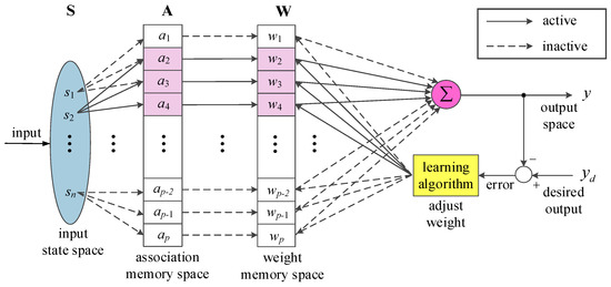
Figure 1.
Schematic diagram of cerebellar model articulation controller mapping.
- Quantization of continuous inputs:
At the beginning of the CMAC action, the quantization step is first performed to quantize the input learning sample into n discrete input states (s1–sn) in order to delimit each input state to a limited closed interval for variation. A higher number of quantization implies a higher learning resolution. Although the arithmetic precision can be increased, thereby increasing the control precision, it consumes relatively more memories; thereby, the arithmetic velocity is reduced, and thus the learning velocity decreases. Therefore, control precision and learning velocity are subjected to a trade-off for the user’s needs.
- 2.
- Mapping of input state space to association memory space:
After the input signal goes through the CMAC quantization step, the quantized input state is mapped to the association memory space. For mapping the input state space to the association memory space, an input state must be mapped to at least two or more association memory addresses, and the association memory addresses mapped by the adjacent input state need to have at least one overlap. The reason why CMAC has to satisfy the aforementioned rules in the input state space mapping to association memory space is mainly that CMAC possesses the ability to infer their similar outputs of unlearned samples through the adjacent memory weights that have been learnt and corrected, i.e., the ability of local generalization.
- 3.
- Mapping of association memory space to weight memory space:
The aim of association memory mapping to weight memory is to correspond the association memory reference state to relevant weight memory. The association memory element in the association memory space is composed of 0 and 1. In simple words, the fired memory addresses are 1, and the remaining memory addresses that are not fired are 0.
- 4.
- Weight memory space to output space:
When the mapping process is completed, the inner products of vector A of association memory and vector W of weight memory are taken as the output values of CMAC, as shown in Equation (4). This is the recall of CMAC, and the weight value will be adjusted and corrected on the basis of the learning algorithm such that the actual output y in the next CMAC learning can be closer to the desired output yd.
where y is the actual output; A is the association memory vector; W is the weight memory vector; p is the number of memory layers; aj is the j-th association memory address; and wj is the j-th weight.
- 5.
- Weight update:
The learning algorithm of CMAC is as shown in Equation (5). It is mainly the error obtained by subtracting the actual output from the desired output. Based on the learning algorithm, errors are fed back to the fired weight in an evenly distributed manner to generate a weight correction amount and correct the original weight value. Training is continuously performed until the output error converges with an allowable range.
The magnitude of learning rate η will greatly influence the learning process. If the learning rate is set to be large, the learning velocity will increase, and the system response will be faster; however, the resulting learning process will considerably change, which leads to system instability. If the learning rate is set to be small, the learning time will be longer, leading to a reduced convergence velocity of the system, and thus the system cannot reach the designated range of convergence in a short time.
3. Adaptive TSK Fuzzy Self-Organizing Recurrent Cerebellar Model Articulation Controller Design
3.1. TSK Fuzzy System
TSK fuzzy rules, also known as functional fuzzy rules, are extended from the Mamdani fuzzy rules. Compared with Mamdani fuzzy rules, there are the following characteristics. In addition, the fuzzy membership function of input s is shown in Figure 2.
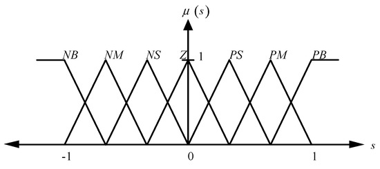
Figure 2.
Membership function of input s.
The TSK fuzzy rules (1) possess high computational efficiency and are suitable for systems with high real-time requirements; (2) they can be combined very well with linear systems, optimized control, and adaptive control systems; and (3) they can guarantee the smoothness of controller outputs.
The difference between TSK fuzzy rules and Mamdani fuzzy rules is that the posterior part of TSK fuzzy rules is a linear combination of input states using the coefficients for linear combination of input states from the online adjusted fuzzy posterior part. The TSK fuzzy rules are as follows:
: if s is NB, then,
: if s is NM, then,
: if s is NS, then,
: if s is Z, then,
: if s is PS, then,
: if s is PM, then,
: if s is PB, then.
If the fuzzy inference adopts the product inference engine, the defuzzification will adopt the center average method. The output is as shown in Equation (6).
where
,
,
,
,
is the degree of membership for the input membership function,
is the linear combination outputs of the posterior part.
3.2. Design of TSK Fuzzy Self-Organizing Recurrent Cerebellar Model Articulation Controller
When CMAC is applied, the number of layers for association memory is fixed. Depending on the input state, the association memory value is 1 when being triggered; when not being triggered, it will be 0. However, such a binary relationship will lower the network resolution and cause the problem of control outputs that are not smooth. This study proposes a self-organizing recurrent cerebellar model articulation controller; the architecture is shown in Figure 3. With the working principle similar to that of a traditional CMAC, the association memory layer is implanted with Gaussian functions to cover the entire input space. Unlike the traditional rectangular function, the Gaussian function possesses the characteristics of being differentiable at any position; therefore, not only can the controller perform function learning but also the resulting outputs can have differential properties. Moreover, similar self-organizing recurrent artificial neural network architecture and adaptive rules are adopted so that the CMAC that is originally static with a fixed number of association memory layers possesses dynamic memory ability and the number of association memory layers can be changed along with the layer decision-making mechanism.
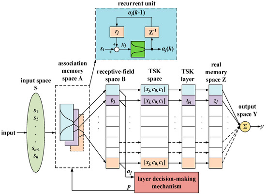
Figure 3.
Takagi–Sugeno–Kang (TSK) fuzzy self-organizing cerebellar model articulation controller architecture.
As shown in Figure 3, the proposed architecture contains an input space S, an association memory space A, a receptive-field space B, a function coupling output space F, real memory space Z, and output space Y. The layer decision-making mechanism of association memory is shown in Figure 4.
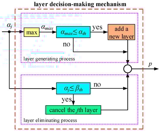
Figure 4.
Layer decision-making mechanism.
The vector of input signals is as shown in Equation (7). It will first be subjected to quantification before entering the TSK fuzzy self-organizing recurrent cerebellar model articulation controller, which takes the range [−1, 1] as the input.
Elements in each input variable vector will be added to the product of the previous association memory output and the recurrent weight, called the recurrent input vector x, as shown in Equations (8) and (9).
where n is the individual number of input states; p is the number of layers in the association memory space; k is the k-th sampling time; and rj is the recurrent weight value. Each variable will correspond to a set of association memories. The pre-set number of layers in the association memory is one layer, and each layer is implanted with one Gaussian function. When the input variable is mapped to each Gaussian function, different degrees of membership αj will be generated, as shown in Equation (10).
where xj is the recurrent input; mj is the midpoint of the Gaussian function; and vj is the standard deviation of the Gaussian function. The membership level αj generated from the association memory layer is individually and correspondingly multiplied and mapped into the receptive field vector b, and the definition of the receptive field vector is shown in Equation (11).
This is expressed in a vector as
where v = [v1, v2,..., vp]T, m = [m1, m2,..., mp]T, and r = [r1, r2,..., rp]T. In this study, the physical memory space is the product of the receptive field space and the TSK output; each recurrent input state xj corresponds to a TSK fuzzy system. Wherein, the fuzzy control rules for the j-th fuzzy system are designed as follows:
b(x,m,v,r) = [b1, b2,…, bp]T,
: if xj is NB, then,
: if xj is NM, then,
: if xj is NS, then,
: if xj is Z, then,
: if xj is PS, then,
: if xj is PM, then,
: if xj is PB, then,
where tjq is the linear combination of the posterior parts in TSK, as shown in Equation (13).
where , for j = 1, 2, …, p. The function value in receptive field vector b is defined as firing strength , which is used for determining the self-organizing layer decision-making mechanism.
αj = bj, for j = 1, 2, …, p.
Next, it is to determine the maximum value αmax from these firing strengths. The maximum firing strength αmax is compared with a preset threshold value αth. If αmax is less than or equal to αth, one new layer of association memory will be added. The threshold value αth is in between 0 and 1.
The determinant of Equation (16) will cause the number of layers to increase by at most one layer at a time, as shown in Equation (17). Newly added association memory is equally implanted with one Gaussian function. For the new Gaussian function, the midpoint , standard deviation , weight , and recurrent weight value are defined as below:
Here, xj is the current input state; vo and ro are the constants given in advance; and wo is the TSK parameter given in advance. If αj is less than or equal to the threshold value βth, the contribution of the layer will not be large, so deleting that layer of association memory will not affect the control performance; thus, the computation amount can be reduced.
The physical memory space is shown by Equation (23).
where j = 1, 2, …, p and q = 1, 2, …, 7. After summation, the resulting total output control amount is as shown in Equation (24).
where Λ = [b1fT, b2fT,..., bpfT]T; W = [, , …, ]T.
αlj ≤ βth.
zj(x, m, v, r, c, f) = tjqbj,
The proposed TFSORC can enable the CMAC with originally static and fixed architecture to possess dynamic memory performance, and the number of association memory layers can increasingly or decreasingly change along with the self-organizing layer decision-making mechanism in order to improve the controller output precision and reduce the computation amount, thereby providing better control performance than the traditional CMAC.
3.3. Design of Adaptive TSK Fuzzy Self-Organizing Recurrent Cerebellar Model Articulation Controller for Chaotic Synchronization Control System
In this study, TFSORC combines the adaptive theorem with an integrated error function along with an improved compensation controller to form the adaptive TSK fuzzy self-organizing recurrent cerebellar model articulation controller (ATFSORC). It takes the signals of integrated error function as the input, as shown in Figure 5. Here, yd is the desired output; y is the actual output; e is the difference value between the desired output and actual output; βw, βm, βv, and βr are the learning rates of weight value for weight memory, midpoint, and standard deviation for Gaussian function, and recurrent weight value, respectively; and γ is the compensation coefficient. The total control amount u of ATFSORC is as shown in Equation (25), where uTFSORC is the control amount of the TSK fuzzy self-organizing cerebellar model articulation controller; and uc is the control amount of the improved compensation controller. When there is an ideal control amount , the error between the uTFSORC of the TSK fuzzy self-organizing cerebellar model articulation controller and the ideal control amount will be compensated by the improved compensation controller uc.
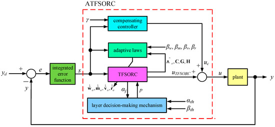
Figure 5.
Adaptive TSK fuzzy self-organizing cerebellar model articulation controller architecture.
In this study, the proposed ATFSORC is used as a synchronization controller for chaotic systems. As shown in Figure 6, the controlled body in Figure 5 is converted into a slave system; yd can be regarded as a master system output (x1, y1); y can be regarded as a slave system output (x2, y2); ex and ey are the error values of x1, x2 and y1, y2, respectively. Moreover, in order to reduce the architectural complexity of ATFSORC, a method of signed distance is introduced to convert the two errors ex and ey in Figure 6 into an error v. Figure 7 shows the ex − ey plane and the switch line LS, which is as shown in Equation (26).
where λ is a normal number; and v is the signed distance between and LS, as shown in Equation (27).
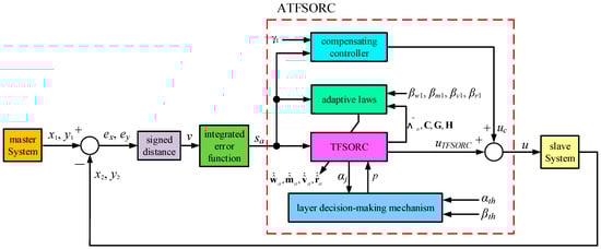
Figure 6.
Adaptive Takagi–Sugeno–Kang (TSK) fuzzy self-organizing recurrent cerebellar model articulation controller (ATFSORC) architecture diagram for chaotic system synchronization.
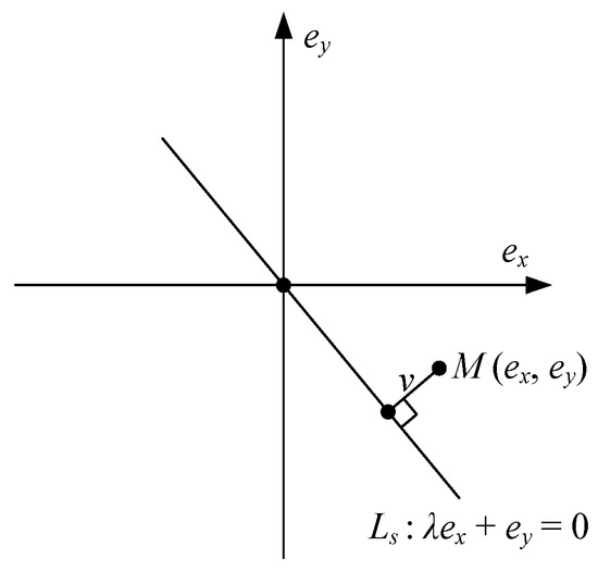
Figure 7.
ex − ey plane of signed distance.
In a neuronal system, a gap junction is an electrical synapse. Through the gap junction, neurons can communicate with each other, and the synaptic current is directly proportional to the membrane potentials between the two neurons. In the previous literature [26], the effect of gap junction on the synchronization of two coupled FitzHugh–Nagumo (FHN) neurons was studied. A circuit diagram of the neuron model is shown in Figure 8, where:
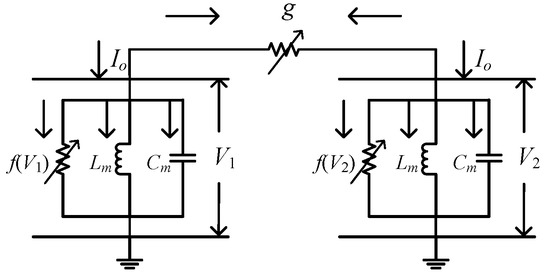
Figure 8.
Circuit diagram of two gap-junction-coupled FitzHugh–Nagumo (FHN) neurons.
V1, V2: Membrane voltages of two gap-junction-coupled neurons,
f(V1), f(V2), Lm, Cm: Electrical parameters of neurons,
g: Coupling strength between neurons,
Io: External electrical stimulation.
The two gap-junction-coupled FHN neuron model is expressed in Equations (28) and (29).
Master system:
Slave system:
First, the errors of two gap-junction-coupled FHN neurons are defined as follows:
Next, the error dynamic system can be expressed as Equation (31).
Merging the two errors of Equation (30) through signed distance into one error v, as shown in Equation (32), we get
Differentiating Equation (32) and substituting in Equation (31) gives Equation (33).
where
,
,
.
In the actual chaos, considering the dynamics of a chaotic system, the parameters will change accordingly under different conditions. Therefore, Equation (32) can be rewritten as
where An and Bn are the nominal values of A and B, respectively; ΔA and ΔB are the variation values of A and B, respectively; and d1 and d2 are the uncertainty dynamic model (system uncertainty), in which d1 = d + Δd, d2 = ΔAv + ΔBu + d1. Then, transposing and arranging the equation, we can obtain
Ideally, if all the parameters of a chaotic system are known, an ideal control amount u* can be constructed.
where v* is the ideal error amount; and k2 is a normal number. Error e is defined as Equation (37).
If the control amount u approaches the ideal control amount u*, Equation (38) can be obtained based on Equations (35) and (36); Equation (39) can be obtained from Equations (37) and (38).
Since k2 is a positive real number and Equation (39) is a strictly Hurwitz polynomial, the error will converge to zero as time passes to infinity, i.e., . Next, the integrated error function sa is defined as in Equation (40).
Differentiating Equation (40) with respect to time t, we get
When the control amount is the ideal control amount u*, the error e can become asymptotically stable. However, in fact, such an ideal control amount cannot be obtained because the system parameters and an unknown dynamic model will vary along with many uncertain factors, and these cannot be known precisely in advance. Therefore, this study proposes ATFSORC, which can use the good approximation capability of a Takagi–Sugeno–Kang (TSK) fuzzy self-organizing recurrent cerebellar model articulation controller (TFSORC) to learn the ideal control amount u* and use the compensation controller to compensate for the error between TFSORC and u*. Figure 6 shows the ATFSORC architecture diagram for chaotic system synchronization. Its output amount is
where u is the total control amount; uTFSORC is the output amount of TFSORC; and uc is the output amount of compensation controller.
Next, the association memory space is partitioned such that the optimal number of stage layers is p*, which is divided into an activated part as p and an inactivated part as . Therefore, the optimal parameters Λ*, W*, m*, v*, and r* are also divided into two parts.
Here, Λ*, W*, m*, v*, and r* are the optimal parameters relative to Λ, W, m, v, and r, respectively; Λa, Wa, ma, va, and ra represent the activated parts, whereas Λi, Wi, mi, vi, and ri represent the inactivated parts.
Based on the universal approximation theorem, it is assumed that there is an optimal output control amount for the TSK fuzzy self-organizing recurrent cerebellar model articulation controller as , and the ideal control amount u* is expressed as Equation (48).
where represents the error between the optimal and ideal controller amount. Since the optimal output control amount cannot be obtained easily, the value is estimated in an iterative manner. That is, the following is assigned:
where are estimated values relative to Λ, W, m, v, and r, respectively. Next, subtracting Equation (35) from Equation (36), we get
By substituting Equations (48) and (49) into the formula, Equation (50) can be rewritten as
where ; .
Through Taylor series, the following expansions can be obtained.
where Ot is a vector of higher-order components. For convenience of derivation, assigning , , and
Then, Equation (52) can be rewritten as
In addition, , so Equation (55) can also be expressed as
Then, substituting Equations (56) and (57) into Equation (51), we get
where D1 is . Assuming that the upper limit of D1 is a normal number δ1,
Theorem 1.
Considering a chaotic synchronization control system as Equation (34), if the synchronization controller is designed to be Equation (49) and while the ATFSORC’s adaptive laws and compensation controller output are as shown from Equation (60) to Equation (64), then the stability of such a controlled system can be guaranteed.
Proof of Theorem 1.
Using the Lyapunov theorem to derive the adaptive laws, the Lyapunov function candidate Vc1 is first defined as follows:
where βw1, βm1, βv1, and βr1 are normal numbers greater than zero. Differentiating Equation (65) and substituting Equation (58) into the equation can give
As Vc1 0, and in order to achieve the goal of , we can assign
Substituting all formulas from Equation (60) to Equation (64) into Equation (66), we get
From Equation (71), as is a negative semi-definite function, there is no guarantee that the error will converge to zero. By using Barbalat’s lemma, we can prove that when time approaches infinity, will approach zero.
The function of Ξ1(t) is defined as follows:
Integrating Equation (72) with respect to time can give Equation (73), where Vc1(t) is as shown in Equation (65).
Since Vc1(0) is bounded, while Vc1(t) is bounded and a non-incremental function, it can be determined from Equation (73) that Ξ1(t) is bounded by time, i.e.,
Next, since Vc1(t) > 0 and , Equation (65) shows that , , , and are bounded. As inferred from Equation (71), when sa ≠ 0, Equation (58) implies that is bounded, and sa is uniformly continuous; therefore, from Equation (72), it is learnt that is bounded, thus proving that is uniformly continuous and is bounded. From Barbalat’s Lemma, we can further obtain the following:
In addition, from Equation (71), when sa = 0, = 0. The above-mentioned inference indicates that for arbitrary sa, when the time t approaches infinity, will converge to zero, and sa at this point will also converge to zero. Equation (41) shows that if an appropriate k2 is selected to conform to the Hurwitz polynomial, the errors e and v will also converge to zero when the time approaches infinity. Through the above derivations, we can ensure that the designed adaptive TSK fuzzy self-organizing recurrent cerebellar model articulation controller system is stable. □
3.4. Design of Improved Compensator
The adaptive TSK fuzzy self-organizing cerebellar model articulation controller proposed in this study contains an improved compensation controller. Equation (64) indicates that the output of compensation controller uc is composed of a normal number δ1 and a sign function of sa, wherein the function of sgn[sa] is defined as in Equation (76). Since δ1 is a normal number, the output of the compensation controller depends on the integrated error function sa value. In fact, there are only three types of states as δ1, 0, and −δ1, which cause the shortcoming of having insufficient transient-state compensation or excessive steady-state compensation.
Therefore, this study proposes an improved compensator to ameliorate the original compensation controller as presented arithmetically in Equation (64). The design of an improved compensation controller focuses on allowing the compensation controller to provide a larger compensation amount in ATFSORC at the transient state and a smaller compensation amount after ATFSORC enters the steady state.
Errors will increase when the compensation amount provided by the compensation controller is insufficient; therefore, the integrated error function sa can be used as the basis to determine whether the ATFSORC has completed learning and entered the steady state. The above-mentioned design concept can be implemented from Equation (77).
where ζ1 is the threshold value for switching the compensation control amount; γ1 is a compensation coefficient; and γ1 > 1, which is used to elastically adjust the magnitude of compensation amount in the transient state. When , it is a transient state, whereas when , it is a steady state. The output amount of the improved compensation controller at the transient state is much larger than that at the steady state, which can effectively ameliorate the shortcoming of poor response of the self-organizing recurrent cerebellar model articulation controller at the transient state. From Equation (77), we see that if the selected δ1 still meets and an appropriate γ1 is selected, the stability of the overall system will not change. Introducing ATFSORC with an improved compensation controller still can guarantee the convergence in errors of the system and maintain the stability of the system.
3.5. Design of Adaptive TSK Fuzzy Self-Organizing Recurrent Cerebellar Model Articulation Controller for Chaotic Stability Control System
In this study, the proposed adaptive TSK fuzzy self-organizing recurrent cerebellar model articulation controller is used as a stability controller for chaotic systems. Therefore, by converting the controlled body in Figure 9 into a chaotic system, yd can be regarded as the chaotic system outputs of x(k) and y(k); y can be regarded as the chaotic system delayed feedback outputs of x(k − 1) and y(k − 1); ex and ey are errors of x(k) − x(k − 1) and y(k) − y(k − 1), respectively. Moreover, in order to reduce the architectural complexity of ATFSORC, the two errors ex and ey are merged into one error v through the signed distance.
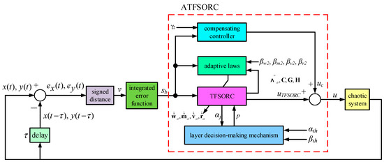
Figure 9.
Architectural diagram of ATFSORC stability controller for chaotic system.
First, the chaotic system is expressed as Equation (78)
After Equation (78) goes through the time delay, Equation (79) can be obtained.
The errors are defined as
Next, the error dynamic system can be expressed as Equation (81).
Merging the two errors of Equation (80) through the signed distance into an error v, we get Equation (82).
Differentiating Equation (82) and substituting Equation (81) into it, we get Equation (83).
where
,
,
.
In an actual chaotic system, considering the dynamics of the chaotic system, the parameters will change accordingly under different conditions. Therefore, Equation (83) can be rewritten as
where An and Bn are the nominal values of A and B, respectively; ΔA and ΔB are the variation values of A and B, respectively; and d1 and d2 are the uncertainty dynamic model (system uncertainty), where d1 = d + Δd and d2 = ΔAv + ΔB(f(t) − f(t − τ) + d1. By transposing and arranging Equation (84), we get
From Equation (85), the proposed ATFSORC output control amount u can be assigned as ; rearranging this can give
Ideally, if all the parameters of the chaotic system are known, an ideal control quantity u* can be constructed as
where v* is the ideal error amount and k3 is a normal number. Error e is defined as Equation (88).
If the control amount u approaches the ideal control amount u*, Equation (89) will be obtained based on Equations (86) and (87), and Equation (90) will be obtained from Equations (88) and (89).
Since k3 is a positive real number, and Equation (90) is a strictly Hurwitz polynomial, the error will converge to zero as time passes to infinity, i.e., . Next, the integrated error function sb is defined as in Equation (91):
Differentiating Equation (91) with respect to time t, we get
When the control amount is an ideal control amount u*, error e can become asymptotically stable. However, in fact, such an ideal control amount cannot be obtained, because system parameters and the unknown dynamic model will vary along with many uncertain factors, and these cannot be known precisely in advance. Therefore, this study proposes ATFSORC that can use the good approximation capability of TFSORC to learn the ideal control amount u*, and use the compensation controller to compensate for the error between TFSORC and u*. Figure 9 is the ATFSORC architectural diagram for chaotic system synchronization; its output is
where u is the total control amount; uTFSORC is the output amount of TFSORC; and uc is the output amount of the compensation controller.
Next, the association memory space is partitioned so that the optimal number of stage layers is p*, which is divided into an activated part as p and an inactivated part as . Therefore, the optimal parameters Λ*, W*, m*, v*, and r* are also divided into two parts.
where Λ*, W*, m*, v*, and r* are the optimal parameters corresponding to Λ, W, m, v, and r, respectively; Λa, Wa, ma, va, and ra represent the activated parts, whereas Λi, Wi, mi, vi, and ri represent the inactivated parts.
Based on the universal approximation theorem, an optimal output control amount for a TSK fuzzy self-organizing recurrent cerebellar model articulation controller, , is assumed, and the ideal control amount u* is expressed as Equation (99).
where represents the error between the two control amounts. Since the optimal output control amount cannot be obtained easily, is estimated in an iterative manner. That is, we assign
where are estimated values corresponding to Λ, W, m, v, and r, respectively. Next, subtracting Equation (86) from Equation (87), we get
Substituting Equations (99) and (100) into the formula, Equation (101) can be rewritten as
where ; .
Through the Taylor series, the following expansions can be obtained.
where Ot is a vector of higher-order components. For convenience of derivation, assigning , , and
then, Equation (103) can be rewritten as
Since , Equation (107) can also be expressed as
Then, substituting Equations (107) and (108) into Equation (102), we get
where . Assuming that the upper limit of D2 is a normal number δ2
Theorem 2.
Considering a chaotic stability control system as Equation (84), if the stability controller is designed to be Equation (100) and the ATFSORC’s adaptive laws and compensation controller output are as shown from Equation (111) to Equation (115), then the stability of such a controlled system can be guaranteed.
Proof of Theorem 2.
Using the Lyapunov theorem to derive the adaptive laws, the Lyapunov function candidate Vc2 is first defined as follows:
where βw2, βm2, βv2, and βr2 are normal numbers greater than zero. By differentiating Equation (116) and substituting Equation (109) into the equation, we get
As Vc2 0 and in order to achieve the goal of , we can assign
Substituting all formulas from Equation (111) to Equation (115) into Equation (117), we get
From Equation (71), as is a negative semi-definite function, there is no guarantee that the error will converge to zero. Using Barbalat’s Lemma, we can prove that when time approaches infinity, approaches zero.
The function Ξ2(t) is defined as follows:
Integrating Equation (123) with respect to time, we get Equation (124), where Vc2(t) is as shown in Equation (116).
Since Vc2(0) is bounded, while Vc2(t) is bounded and a non-incremental function, it can be determined from Equation (124) that Ξ2(t) is bounded by time, i.e.,
Next, since Vc2(t) > 0 and , Equation (116) shows that , , , and are bounded. As inferred from Equation (122) that when sb ≠ 0, from Equation (109), we see that is bounded and sb is uniformly continuous; Equation (122) shows that is bounded, thus proving that is uniformly continuous and is bounded. From Barbalat’s Lemma, we can further obtain the following.
From Equation (122), we see that when sb = 0, = 0. From the above-mentioned inference, it can be learnt that for arbitrary sb, when the time t approaches infinity, will converge to zero, and sb at this point of time will also converge to zero. Equation (92) shows that if an appropriate k3 is selected to conform to the Hurwitz polynomial, the error e and v will also converge to zero when the time approaches infinity. Through the above derivations, we can ensure that the designed adaptive TSK fuzzy self-organizing recurrent cerebellar model articulation controller system is stable. □
3.6. Design of Improved Compensator
The adaptive TSK fuzzy self-organizing cerebellar model articulation controller proposed in this study contains an improved compensation controller. From Equation (115), the output of compensation controller uc is composed of a normal number δ2 and a sign function of sb, wherein the function of sgn[sb] is defined as in Equation (127). Since δ2 is a normal number, the output of the compensation controller depends on the integrated error function sb value. In fact, there are only three types of states as δ2, 0, and −δ2, which cause the shortcoming of insufficient transient-state compensation or excessive steady-state compensation.
Therefore, this study proposes an improved compensator to ameliorate the original compensation controller as presented arithmetically in Equation (115). Design of the improved compensation controller focuses on allowing the compensation controller to provide a larger compensation amount in ATFSORC at the transient state and a smaller compensation amount after ATFSORC enters the steady state.
Errors will increase when the compensation amount provided by the compensation controller is insufficient; therefore, the integrated error function sb can be used as the basis to determine whether ATFSORC has completed learning and entered the steady state. The above-mentioned design concept can be implemented from Equation (128).
where ζ2 is the threshold value for switching compensation control quantity; γ2 is a compensation coefficient; and γ2 > 1, which is used to elastically adjust the magnitude of compensation amount at the transient state. When , it is a transient state, while when , it is a steady state. Furthermore, the output amount of the improved compensation controller at the transient state is considerably larger than that at the steady state, which can effectively ameliorate the shortcoming of poor response of the self-organizing recurrent cerebellar model articulation controller at the transient state. By observing (128), note that if the selected δ2 still meets and an appropriate γ2 is selected, the stability of the overall system will not change. Introducing ATFSORC with an improved compensation controller can still guarantee the convergence in errors of the system and maintain the stability of the system.
4. Simulation Results and Analysis on Chaotic Synchronization and Stability Control
In this study, the proposed ATFSORC was applied on the synchronization control of chaotic systems, and it was compared with CMAC and fuzzy CMAC (FCMAC) to validate the control performance of the proposed ATFSORC. Relevant parameters for simulation are shown in Table 2. At the beginning of the simulation, a trial-and-error method was used to find a set of initial values of controller parameters that can enable the system to run smoothly. After that, all the controller parameters were subjected to simulation using these initial values. The simulation contains the following two scenarios:
Table 2.
Simulation parameters for the synchronization control of chaotic systems.
- By adjusting the coupling strength g of the gap junction in Equations (28) and (29) to 0.01 and 1 as well as by changing the cut-in control time point of ATFSORC to 300 s after the chaotic system running, the simulation would validate the feasibility of the controller proposed in this study.
- By comparing the response data of ATFSORC with those of CMAC and FCMAC, the controller performance was determined via root mean square errors and average errors.
Figure 10 and Figure 11 show the uncontrolled chaotic system response diagrams for coupling strengths g = 0.01 and g = 1, respectively. To observe the unpredictable behavior of the chaotic system, the control amount u for the chaotic system in Equation (29) was set to zero, and the initial condition was set to (x1, x2, y1, y2) = (1, 0, 1, 0). Figure 10a and Figure 11a show the phase diagrams of the master system. The phase diagrams show that the master system indeed operates at a chaotic state. Figure 10b and Figure 11b show the phase diagrams of the slave system, which has different initial starting points from those of the master system; thus, the diagrams demonstrate the characteriztics of chaos and have phase plane trajectories different from those of the master system. Figure 10c shows a phase diagram constructed by x1 and x2. As shown very clearly from the diagram, when the primary and secondary systems are asynchronous, the entire phase plane trajectory is disorganized and in disorder. Figure 11c shows a phase diagram constructed by x1 and x2. As shown very clearly from the diagram, when the primary and secondary systems are asynchronous, the entire phase plane is slightly disorganized; however, due to the large coupling strength, the x coefficients of the master–slave system will gradually synchronize. Figure 10d shows a phase diagram constructed by y1 and y2. Similarly, we can clearly discover that when the control amount is zero, the asynchronous state is presented. Figure 11d shows the phase diagram constructed of y1 and y2. We can similarly discover that due to the large coupling strength, the y coefficient for the master–slave system will gradually synchronize.
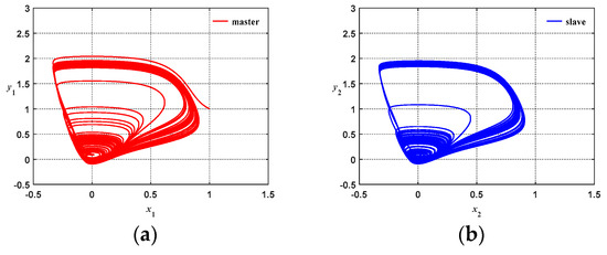
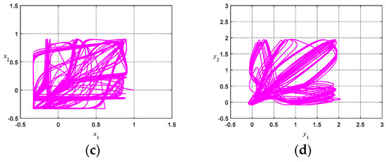
Figure 10.
Uncontrolled coupled nonlinear chaotic system (g = 0.01): (a) Master system phase diagram; (b) Slave system phase diagram; (c) x1, x2 phase diagram; (d) y1, y2 phase diagram.
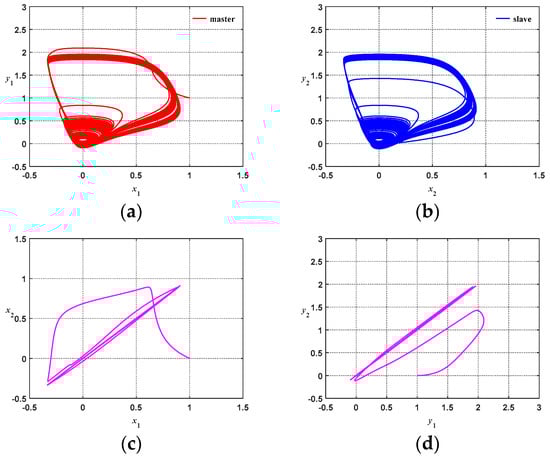
Figure 11.
Uncontrolled coupled nonlinear chaotic system (g = 1): (a) Master system phase diagram; (b) Slave system phase diagram; (c) x1, x2 phase diagram; (d) y1, y2 phase diagram.
Figure 12 and Figure 13 show the response diagrams of chaotic system synchronization for ATFSORC with coupling strengths of g = 0.01 and g = 1, respectively; initial conditions were set as (x1, x2, y1, y2) = (1, 0, 1, 0). Figure 12a and Figure 13a show the phase diagrams of the master system, starting from the coordinate at (1, 1) and performing a chaotic counterclockwise trajectory motion. Figure 12b and Figure 13b show the phase diagram of the slave system, starting from the coordinates at (0, 0); it can be seen that after inserting the controller, the slave system can rapidly catch up with the trajectory of the master system. Figure 12c and Figure 13c show the phase diagrams for x1 and x2. The observation shows that due to the addition of ATFSORC, the x parameters for the master–slave system can be synchronized in a short period of time, demonstrating excellent control performance. Figure 12d and Figure 13d show the phase diagrams for y1 and y2; we can observe that the slave system can be rapidly synchronized with the master system. Figure 12e and Figure 12f show the response diagram and errors for x1 and x2, respectively. The observation implies that the master–slave system can be fully synchronized in about 9 s, and the error after the steady state is almost approaching zero. Figure 13e,f are the response diagram and errors for x1 and x2, respectively. The observation shows that the master–slave system can be fully synchronized in about 9 s, and the error after the steady state is almost approaching zero. Figure 12g,h show the response diagram and errors for y1 and y2. In the same manner, it can be observed that the synchronization can be complete in about 9 s, and the steady-state error approaches zero. Looking coordinately with the number of associate memory layers in Figure 12i,j, it is found that because the transient error is larger, the number of layers is increased from the preset one layer to six layers only within 0.3 s, the number of layers is increased layer by layer, and the number of association memory layers at the steady state is fixed as 7 layers. Figure 13g,h show the response diagram and errors for y1 and y2. In the same manner, it can be observed that the synchronization can be completed in about 9 s, and the steady-state error approaches zero. Looking coordinately with the number of associate memory layers in Figure 13i,j, it can be found that because the transient error is larger, the number of layers increases from the preset one layer to six layers only within 0.2 s, and the number of association memory layers at steady state is fixed as seven layers. Figure 12k and Figure 13k show the response diagrams of all control amounts of ATFSORC, wherein adding the improved compensation controller output uc on the TSK fuzzy self-organizing recurrent cerebellar model articulation controller output will be equal to the control amount u in Equation (29).
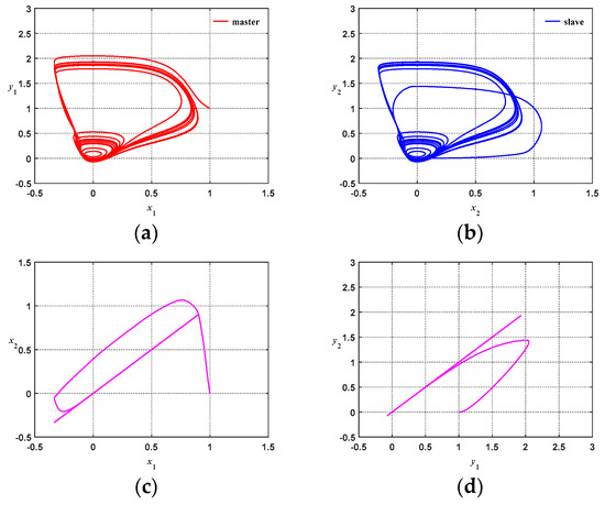
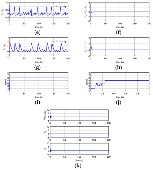
Figure 12.
Simulation results of ATFSORC chaotic system synchronization control (g = 0.01): (a) Master system phase diagram for ATFSORC; (b) Slave system phase diagram for ATFSORC; (c) x1, x2 phase diagram for ATFSORC; (d) y1, y2 phase diagram for ATFSORC; (e) x1, x2 response for ATFSORC; (f) Error ex for ATFSORC; (g) y1, y2 response for ATFSORC; (h) Error ey for ATFSORC; (i) Number of association memory layers for ATFSORC; (j) Number of association memory layers for ATFSORC (partial); (k) Control amount for ATFSORC.
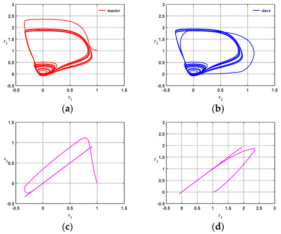
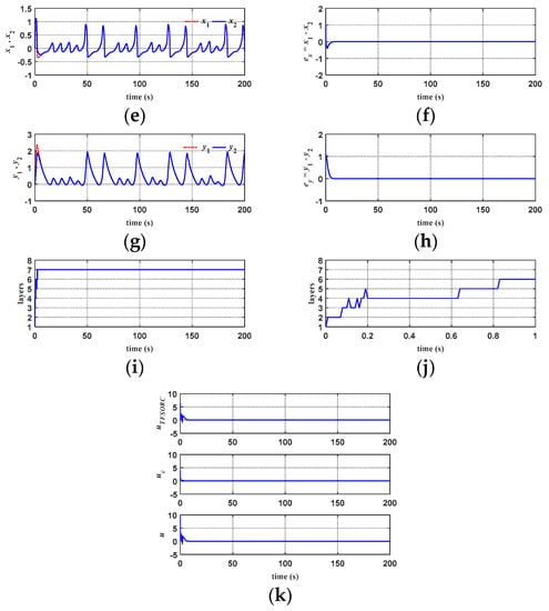
Figure 13.
Simulation results of ATFSORC chaotic system synchronization control (g = 1): (a) Master system phase diagram for ATFSORC; (b) Slave system phase diagram for ATFSORC; (c) x1, x2 phase diagram for ATFSORC; (d) y1, y2 phase diagram for ATFSORC; (e) x1, x2 response for ATFSORC; (f) Error ex for ATFSORC; (g) y1, y2 response for ATFSORC; (h) Error ey for ATFSORC; (i) Number of association memory layers for ATFSORC; (j) Number of association memory layers for ATFSORC (partial); (k) Control amount for ATFSORC.
Figure 14 shows the response diagrams of the chaotic system for ATFSORC, wherein the coupling strength g = 0.01 and g = 1; the chaotic system is first allowed to run for 300 s before the controller cuts in, and the initial conditions are set as (x1, x2, y1, y2) = (1, 0, 1, 0). Figure 14a,b show the x1, x2 response and y1, y2 response for ATFSORC, respectively. We can see that the master–slave system is at an asynchronous stage before 300 s; after approximately 6 s, the controller cuts in, and the slave system can keep up with the master system trajectory. Figure 14c,d show errors ex and ey, respectively. Looking coordinately with the number of association memory layers and their partial enlarged views in Figure 14e,f, it is found that because the errors at the transient state are larger, the number of layers is added from the preset one layer to six layers only within 0.25 s; after 0.5 s, since the error is smaller, the number of layers is reduced by one layer. Figure 14g shows the response diagram of all the control amount for ATFSORC, wherein adding the improved compensation controller output uc on the TSK fuzzy self-organizing recurrent cerebellar model articulation controller output will be equal to the control amount u in Equation (29).
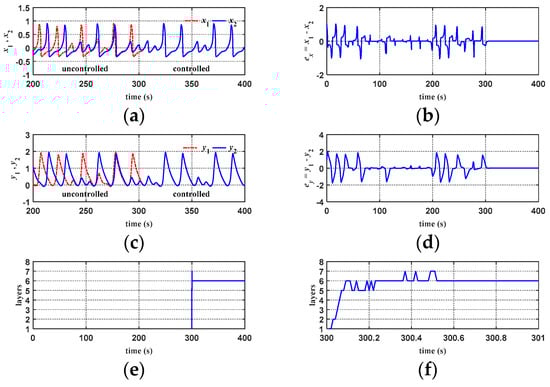
Figure 14.
Simulation results of ATFSORC chaotic system synchronization control (g = 0.01, Cut-in control at 300 sec): (a) x1, x2 response for ATFSORC; (b) error ex for ATFSORC; (c) y1, y2 response diagram for ATFSORC; (d) Error ey for ATFSORC; (e) Number of association memory layers for ATFSORC; (f) Number of association memory layers for ATFSORC (partial); (g) Control amount for ATFSORC.
Figure 15 compares the response diagrams of chaotic system synchronization for ATFSORC, FCMAC, and CMAC, with a coupling strength of g = 0.01 and an initial condition set as (x1, x2, y1, y2) = (1, 0, 1, 0). Figure 15a–c show comparisons of response diagrams for the master systems; Figure 15d–f show comparisons of response diagrams for the slave systems. The comparisons show that although all the slave systems can catch up with the trajectories of the master systems, the trajectory jittering phenomena of CMAC and FCMAC at the transient state is more obvious than that of ATFSORC. Figure 15g–i show comparisons of the x1 and x2 phase diagrams. Under the ideal circumstance, when the steady-state error is 0, i.e., x1 is equal to x2, the phase diagram should present a strip of a straight line; the line strip from CMAC is thicker, and its transient time is longer; FCMAC is second, and ATFSORC is the best. Figure 15j–l show comparisons of the y1 and y2 phase diagrams. Under the ideal circumstance, when the steady-state error is 0, i.e., y1 is equal to y2, the phase diagram should present a strip of a straight line; the comparisons show that the line strip of CMAC is thicker and the transient time is longer, FCMAC is second, and ATFSORC is the best.
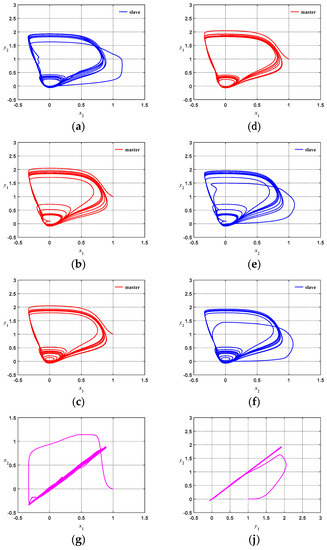
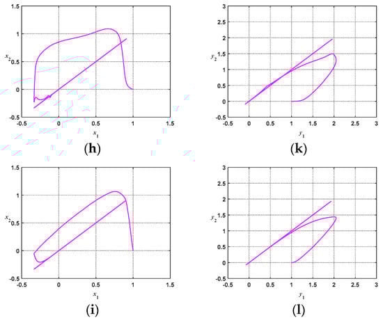
Figure 15.
Comparisons on simulation results of chaotic system synchronization control (g = 0.01): (a) Master system phase diagram for cerebellar model articulation controller (CMAC); (b) Master system phase diagram for fuzzy CMAC (FCMAC); (c) Master system phase diagram for ATFSORC; (d) Slave system phase diagram for CMAC; (e) Slave system phase diagram for FCMAC; (f) Slave system phase diagram for ATFSORC; (g) x1, x2 phase diagram for CMAC; (h) x1, x2 phase diagram for FCMAC; (i) x1, x2 phase diagram for ATFSORC; (j) y1, y2 phase diagram for CMAC; (k) y1, y2 phase diagram for FCMAC; (l) y1, y2 phase diagram for ATFSORC.
Figure 16 compares the response diagrams of chaotic system synchronization for AFSSORC, FCMAC, and CMAC, with a coupling strength of g = 1 and the initial condition set as (x1, x2, y1, y2) = (1, 0, 1, 0). Figure 16a–c show comparisons of the master systems’ response diagrams. Figure 16d–f show comparisons of the slave systems’ response diagrams. The comparisons indicate that although all the slave systems can catch up with the trajectories of the master systems, the trajectory jittering phenomena of CMAC and FCMAC at the transient state are more obvious than that of ATFSORC. Figure 16g–i show comparisons of the x1 and x2 phase diagrams. Under the ideal circumstance, when the steady-state error is 0, i.e., x1 is equal to x2, the phase diagram should present a strip of a straight line. The comparisons show that the CMAC line strip is thicker and the transient time is longer, FCMAC is second, and ATFSORC is the best. Figure 16j–l show comparisons of y1 and y2 phase diagrams. Under the ideal circumstance, when the steady-state error is 0, i.e., y1 is equal to y2, the phase diagram should present a strip of a straight line. The comparison shows that the transient time for CMAC is longer, FCMAC is second, and ATFSORC is the best. Figure 16m–o show comparisons of the x1 and x2 response diagram. Coordinating with the comparisons of error ex from Figure 16p–r, we can see that although all the slave systems can catch up with the trajectories of the master systems, the steady-state error of CMAC lies between −0.002 and 0.002, and the steady-state error of FCMAC lies between −0.0002 and 0.0002, whereas the steady-state error of ATFSORC is almost 0. Therefore, the proposed ATFSORC error is smaller and the convergence velocity is faster.
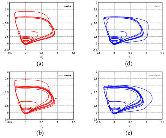
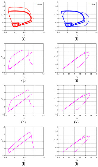
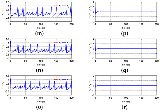
Figure 16.
Comparisons on simulation results of chaotic system synchronization control (g = 1): (a) Master system phase diagram for CMAC; (b) Master system phase diagram for FCMAC; (c) Master system phase diagram for ATFSORC; (d) Slave system phase diagram of CMAC; (e) Slave system phase diagram for FCMAC; (f) Slave system phase diagram for ATFSORC; (g) x1, x2 phase diagram for CMAC; (h) x1, x2 phase diagram for FCMAC; (i) x1, x2 phase diagram for ATFSORC; (j) y1, y2 phase diagram for CMAC; (k) y1, y2 phase diagram for FCMAC; (l) y1, y2 phase diagram for ATFSORC; (m) x1, x2 response for CMAC; (n) x1, x2 response for FCMAC; (o) x1, x2 response for ATFSORC; (p) Error ex for CMAC; (q) Error ex for FCMAC; (r) Error ex for ATFSORC.
Figure 17 compares the response diagrams of chaotic system synchronization for ATFSORC, FCMAC, and CMAC, with a coupling strength of g = 0.01 and g = 1. Moreover, the chaotic system is first allowed to run for 300 s before the controller cuts in, and the initial conditions are set as (x1, x2, y1, y2) = (1, 0, 1, 0). Figure 17a–c show comparisons of x1 and x2 response diagrams. To demonstrate the characteristics of chaos, the controller is first removed after the system is run for 300 s; then, the controller cuts in, thereby validating the performance of the controller. The results show that all the slave systems’ trajectories can keep up with the master systems’ trajectories, but the steady-state response of ATFSORC is better than those of CMAC and FCMAC. Figure 17d–f show comparisons of error ex. The steady-state errors lie between −0.002 and 0.002 for CMAC and between −0.0002 and 0.0002 for FCMAC, whereas the steady-state error of ATFSORC is almost 0; therefore, the proposed ATFSORC performance is better. Figure 17g–i show a comparison of y1 and y2 response diagrams. To demonstrate the characteristics of chaos, the controller is first removed after the system is run for 300 s, and then the controller cuts in, thereby validating the performance of the controller. The results show that all the slave systems’ trajectories can keep up with the master systems’ trajectories, but the steady-state response of ATFSORC is better than those of CMAC and FCMAC. Figure 17j–l show comparisons of the error ey. The steady-state error of CMAC lies between −0.002 and 0.002, and that of FCMAC lies between −0.0002 and 0.0002; in contrast, the steady-state error of ATFSORC is almost 0. Therefore, the proposed ATFSORC performance is better.
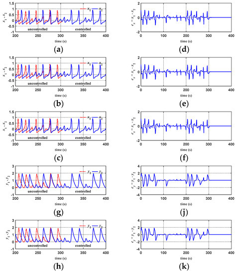
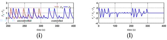
Figure 17.
Comparisons on simulation results of chaotic system synchronization control (g = 0.01, cut-in control at 300 sec): (a) x1, x2 response for CMAC; (b) x1, x2 response for FCMAC; (c) x1, x2 response for ATFSORC; (d) Error ex for CMAC; (e) Error ex for FCMAC; (f) Error ex for ATFSORC; (g) y1, y2 response for CMAC; (h) y1, y2 response for FCMAC; (i) y1, y2 response for ATFSORC; (j) Error ey for CMAC; (k) Error ey for FCMAC; (l) Error ey for ATFSORC.
The proposed ATFSORC was applied on the stability control of a chaotic system, and it was compared with CMAC and FCMAC to validate the control performance of the proposed ATFSORC. Relevant parameters for simulations are shown in Table 3. At the beginning of the simulation, a set of initial values of controller parameters that allow the system to run smoothly was found by trial and error. These initial values were taken for all the controller parameters for simulation. Simulations contain the following two scenarios:
Table 3.
Parameters of chaotic system stability simulation.
- In the simulation, the controller will first be removed; control will cut in after the chaotic system has run for 400 s; thereby, the feasibility of the controller is validated.
- Response data of ATFSORC will be controlled with those of CMAC and FCMAC to observe the stabilization time.
Figure 18 shows the stability simulation results of a chaotic system for ATFSORC. In Figure 18a, to observe the characteristics of a chaotic system, the control amount of the chaotic system is set as zero, and the initial condition is set as (x, y) = (0, 0). Figure 18b shows the stable phase diagram for the chaotic system. The controller cuts in at 400 s, and the trajectory of the last 100 s is plotted. It is observed that the proposed ATFSORC can immediately control the chaotic system to a stable state of period one in a short time; the phase plane presents a periodic closed trajectory. Figure 18c,e show the x response diagram for ATFSORC and the y response diagram for ATFSORC, respectively. After cut-in control at 400 s, the chaotic system can be stabilized in a short time, and the trajectory presents a periodic variation. Figure 18d,f show error ex for ATFSORC and error ey for ATFSORC, respectively. The coordination of the number of association memory layers in Figure 18g indicate that due to the larger transient error when the controller cuts in at 400 s, the number of associative memory layers is increased from the preset one layer to four layers within only 4 s, and then, five layers is fixed after entering the steady state. Figure 18h is a partial enlarged view on the number of association memory layers. Figure 18i is a response diagram of all control amounts for ATFSORC.
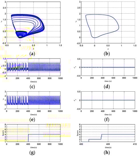
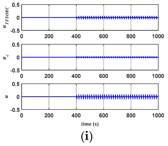
Figure 18.
Simulation results of ATFSORC chaotic system stability control: (a) Phase diagram for uncontrolled chaotic system; (b) Stable phase diagram for ATFSORC; (c) x response for ATFSORC; (d) Error ex for ATFSORC; (e) y response for ATFSORC; (f) Error ey for ATFSORC; (g) Number of association memory layers for ATFSORC; (h) Number of association memory layers for ATFSORC (partial); (i) Control amount for ATFSORC.
Figure 19 shows comparisons on the response diagrams of chaotic system stability for CMAC, FCMAC, and ATFSORC, wherein the control amount at the beginning is set as zero with cut-in control after 400 s. Figure 19a–c show the phase diagrams of uncontrolled chaotic systems. The aim is to display the characteristics of a trajectory repeat of the chaotic system. The coordination with the stability phase diagrams from Figure 19d–f shows a clear comparison of the difference before and after control. Figure 19g–i show the x response diagrams of CMAC, FCMAC, and ATFSORC. Figure 19g shows that CMAC cuts in control at 400 s and the x response should stabilize the periodic variation at about 500 s. Figure 19h indicates that FCMAC cuts in control at 400 s, and the x response should be able to stably present periodic variation in a very short time. From Figure 19i, we can see that the ATFCMAC cuts in control at 400 s, and the x response should be able to stably present the closed trajectory of period one almost immediately. Figure 19j–l show the error ex for CMAC, FCMAC, and ATFSORC. Figure 19m–o show the y response diagrams for CMAC, FCMAC, and ATFSORC. Figure 19m shows that CMAC cuts in control at 400 s, and y response should stabilize the periodic variation at about 500 s. Figure 19n shows that FCMAC cuts in control at 400 s, and the y response should be able to stably present periodic changes in a very short time. From Figure 19o, we can see that the ATFCMAC cuts in control at 400 s, and the y response should be able to stably present the closed trajectory of period one almost immediately. Figure 19p–r show the error ey for CMAC, FCMAC, and ATFSORC. From the simulation results, we know that the proposed ATFSORC possess good control performance and is suitable to be applied on the control and synchronization of chaotic systems.
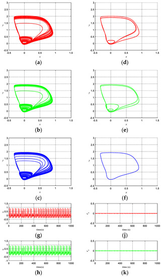
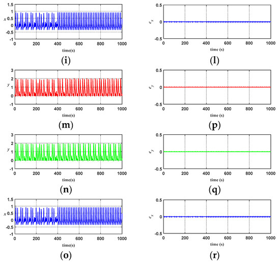
Figure 19.
Comparisons on simulation results of chaotic system stability control: (a) Phase diagram of uncontrolled chaotic system; (b) Phase diagram of uncontrolled chaotic system; (c) Phase diagram of uncontrolled chaotic system; (d) Stable phase diagram for CMAC; (e) Stable phase diagram for FCMAC; (f) Stable phase diagram for ATFSORC; (g) x response for CMAC; (h) x response for FCMAC; (i) x response for ATFSORC; (j) Error ex for CMAC; (k) Error ex for FCMAC; (l) Error ex for ATFSORC; (m) y response for CMAC; (n) y response for FCMAC; (o) y response for ATFSORC; (p) Error ey for CMAC; (q) Error ey for FCMAC; (r) Error ey for ATFSORC.
5. Conclusions
In this study, the TSK fuzzy system and recurrent cerebellar model with a self-organizing architecture are introduced into a cerebellar model controller in combination with an integrated error function and an improved compensation controller to design an adaptive TSK fuzzy self-organizing recurrent cerebellar model controller, ATFSORC. By adopting self-organizing and recurrent artificial neural network architecture, CMAC could possess dynamic state and parameter correction capabilities, in which the number of association memory layers can be modulated in accordance with the layer decision-making mechanism, thereby achieving better control response and the robustness resisting external disturbance. Simulation results show that when the proposed ATFSORC is applied to the synchronization and stability control of chaotic system, it possesses superior control performance when the parameters of the chaotic system or the cut-in control time point change. Furthermore, the simulation results also demonstrate that the proposed ATFSORC has better control performance in comparison with the FCMAC and CMAC.
For future research studies, it is expected that the proposed ATFSORC may have better dynamic response characteristics when combining with other advanced control theories such as function links, wavelet analysis, Petri net, etc. Moreover, the synchronization and stability control of a chaotic system proposed in this study may also be applied in conjunction with other advanced control theories for daily life applications such as the chaotic synchronous control of the number of vehicles on the highway and its gateways, cardiac pacemaker control to ensure the stabilization of heart beat frequency within a certain range under various physical conditions, etc.
Author Contributions
Contribution of each author is the same. All authors have read and agreed to the published version of the manuscript.
Funding
This research received no external funding.
Institutional Review Board Statement
Not applicable.
Informed Consent Statement
Not applicable.
Data Availability Statement
Not applicable.
Conflicts of Interest
The authors declare no conflict of interest.
References
- Lorenz, E.N. Deterministic nonperiodic flow. J. Atmos. Sci. 1963, 20, 130–141. [Google Scholar] [CrossRef]
- Liu, J.; Sprott, J.C.; Wang, S.; Ma, Y. Simplest chaotic system with a hyperbolic sine and its applications in DCSK scheme. IET Commun. 2018, 12, 809–815. [Google Scholar] [CrossRef]
- Liu, Y.; Park, J.H.; Guo, B.Z.; Shu, Y. Security-enhanced electro-optic feedback phase chaotic system based on nonlinear coupling of two delayed interfering branches. IEEE Trans. Fuzzy Syst. 2018, 26, 1040–1045. [Google Scholar] [CrossRef]
- Wang, C.; Ji, Y.; Wang, H.; Bai, L. Further results on stabilization of chaotic systems based on fuzzy memory sampled-data control. IEEE Photon. J. 2018, 10, 655–663. [Google Scholar]
- Hua, Z.; Zhou, B.; Zhou, Y. Sine-transform-based chaotic system with FPGA implementation. IEEE Trans. Ind. Electron. 2018, 65, 2557–2566. [Google Scholar] [CrossRef]
- Tao, H.T.; Wang, J.; Deng, B.; Wei, X.L.; Chen, Y.Y. Adaptive synchronization control of coupled chaotic neurons in an external electrical stimulation. Chin. Phys. B 2013, 22, 058701. [Google Scholar]
- Hsu, C.F. Hermite-neural-network-based adaptive control for a coupled nonlinear chaotic system. Neural. Comput. Appl. 2013, 22, 421–433. [Google Scholar] [CrossRef]
- Lin, F.J.; Lu, K.C.; Yang, B.H. Recurrent fuzzy cerebellar model articulation neural network based power control of a single-stage three-phase grid-connected photovoltaic system during grid faults. IEEE Trans. Ind. Electron. 2017, 64, 1258–1268. [Google Scholar] [CrossRef]
- Che, Y.Q.; Wang, J.S.; Zhou, S.; Deng, B. Robust synchronization control of coupled chaotic neurons under external electrical stimulation. Chaos Solitons Fractals 2009, 40, 1333–1342. [Google Scholar] [CrossRef]
- Wu, C.W.; Hsu, C.F.; Hwang, C.K. Master–slave chaos synchronization using adaptive TSK-type CMAC neural control. J. Frankl. Inst. 2011, 348, 1847–1868. [Google Scholar] [CrossRef]
- Wen, C.M.; Cheng, M.Y. Development of a recurrent fuzzy CMAC with adjustable input space quantization and self-tuning learning rate for control of a dual-axis piezoelectric actuated micromotion stage. IEEE Trans. Ind. Electron. 2013, 60, 5105–5115. [Google Scholar] [CrossRef]
- Lin, C.M.; Li, H.Y. TSK fuzzy CMAC-based robust adaptive backstepping control for uncertain nonlinear systems. IEEE Trans. Fuzzy Syst. 2012, 20, 1147–1154. [Google Scholar] [CrossRef]
- Lian, R.J. Enhanced adaptive self-organizing fuzzy sliding-mode controller for active suspension systems. IEEE Trans. Ind. Electron. 2013, 60, 958–968. [Google Scholar] [CrossRef]
- Lin, C.M.; Li, H.Y. Self-organizing adaptive wavelet CMAC backstepping control system design for nonlinear chaotic systems. Nonlinear Anal. Real World Appl. 2013, 14, 206–223. [Google Scholar] [CrossRef]
- Chen, C.S. TSK-type self-organizing recurrent-neural-fuzzy control of linear microstepping motor drives. IEEE Trans. Power Electron. 2010, 25, 2253–2265. [Google Scholar] [CrossRef]
- Che, Y.Q.; Cui, S.G.; Wang, J.; Deng, B.; Wei, X.L. Chaos synchronization of coupled FitzHugh-Nagumo neurons via adaptive sliding mode control. In Proceedings of the Third International Conference on Measuring Technology and Mechatronics Automation, Shanghai, China, 6–7 January 2011. [Google Scholar]
- Peng, Y.F.; Lin, C.M. Adaptive recurrent cerebellar model articulation controller for linear ultrasonic motor with optimal learning rates. Neurocomputing 2007, 70, 2626–2637. [Google Scholar] [CrossRef]
- Hung, Y.C.; Lin, F.J.; Hwang, J.C. Wavelet fuzzy neural network with asymmetric membership function controller for electric power steering system via improved differential evolution. IEEE Trans. Power Electron. 2015, 30, 2350–2362. [Google Scholar] [CrossRef]
- Lin, C.M.; Li, H.Y. A novel adaptive wavelet fuzzy cerebellar model articulation control system design for voice coil motors. IEEE Trans. Ind. Electron. 2012, 59, 2024–2033. [Google Scholar] [CrossRef]
- Li, S.; Zhou, M.; Yu, X. Design and implementation of terminal sliding mode control method for PMSM speed regulation system. IEEE Trans. Industr. Inform. 2013, 9, 1879–1891. [Google Scholar] [CrossRef]
- Lin, F.J.; Lee, S.Y.; Chou, P.H. Computed force control system using functional link radial basis function network with asymmetric membership function for piezo-flexural nanopositioning stage. IET Control Theory Appl. 2013, 7, 2128–2142. [Google Scholar] [CrossRef]
- Lin, F.J.; Lu, K.C.; Ke, T.H.; Yang, B.H.; Chang, Y.R. Reactive power control of three-phase grid-connected PV system during grid faults using Takagi–Sugeno–Kang probabilistic fuzzy neural network control. IEEE Trans. Ind. Electron. 2015, 62, 5516–5528. [Google Scholar] [CrossRef]
- Albus, J.S. New approach to manipulator control: The cerebellar model articulation controller (CMAC). J. Dyn. Sys. Meas. Control. 1975, 97, 220–227. [Google Scholar] [CrossRef]
- Wang, Z.Q.; Schiano, J.L.; Ginsberg, M. Hash-coding in CMAC neural networks. IEEE Int. Conf. Neural Netw. 1996, 3, 1698–1703. [Google Scholar]
- Sahoo, S.K.; Panda, S.K.; Xu, J.X. Iterative learning-based high-performance current controller for switched reluctance motors. IEEE Trans. Energy Convers. 2004, 19, 491–497. [Google Scholar] [CrossRef]
- Chuang, C.H.; Lin, Y.H.; Wang, C.H.; Hsu, C.F. Synchronization of two coupled neurons using CMAC neural networks. In Proceedings of the International Conference on Machine Learning and Cybernetics, Guilin, China, 10–13 July 2011; pp. 789–794. [Google Scholar]
Publisher’s Note: MDPI stays neutral with regard to jurisdictional claims in published maps and institutional affiliations. |
© 2021 by the authors. Licensee MDPI, Basel, Switzerland. This article is an open access article distributed under the terms and conditions of the Creative Commons Attribution (CC BY) license (http://creativecommons.org/licenses/by/4.0/).