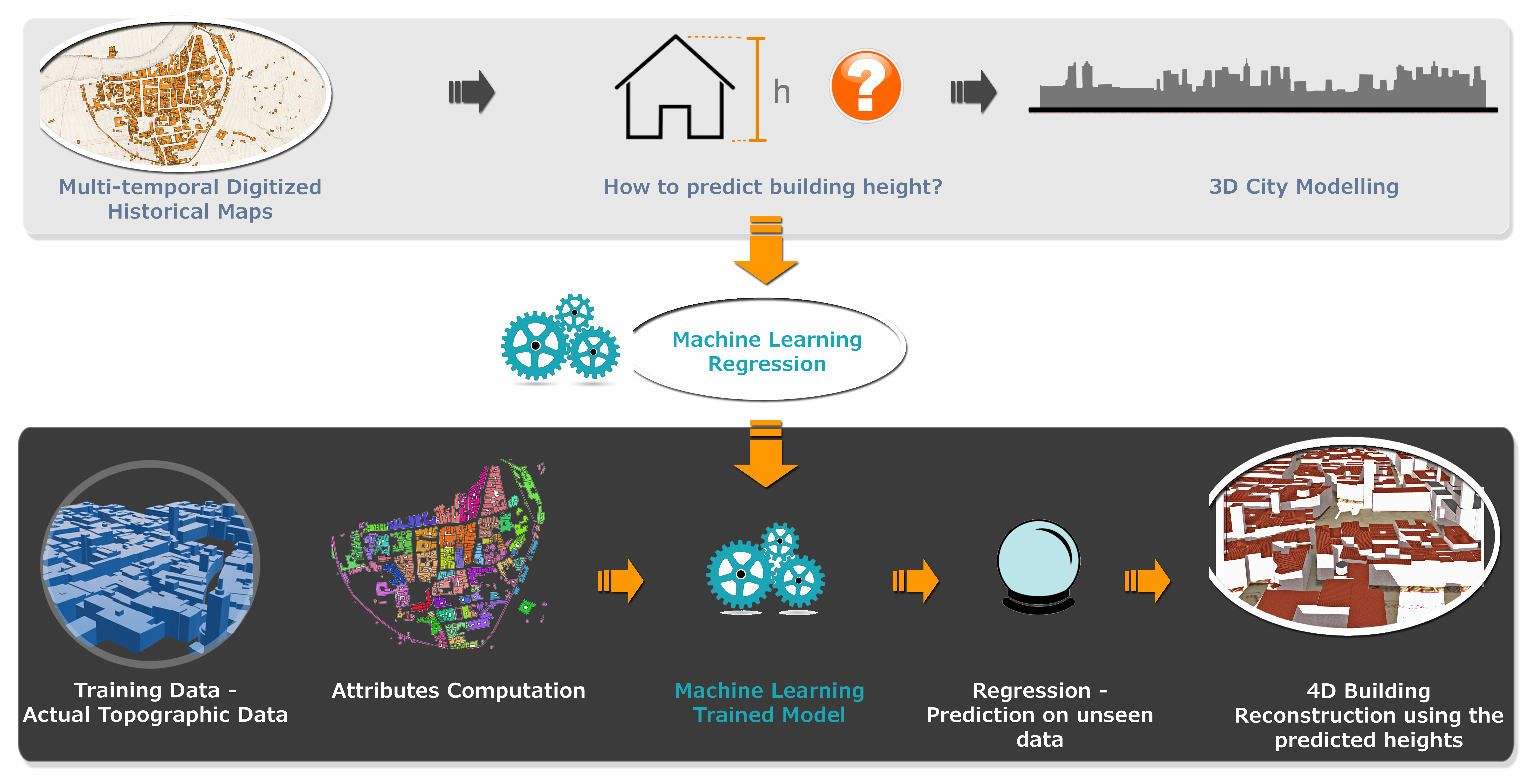
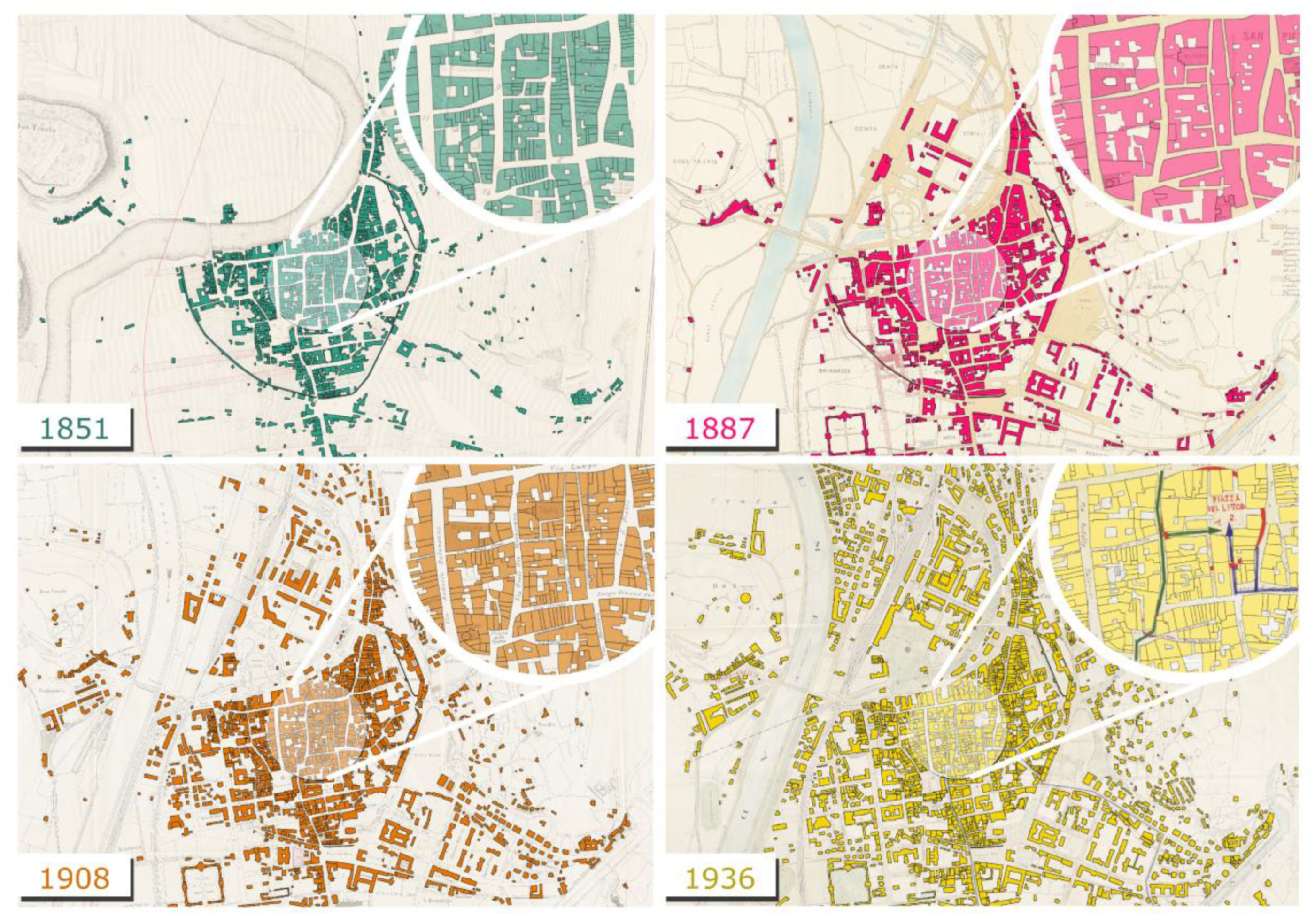
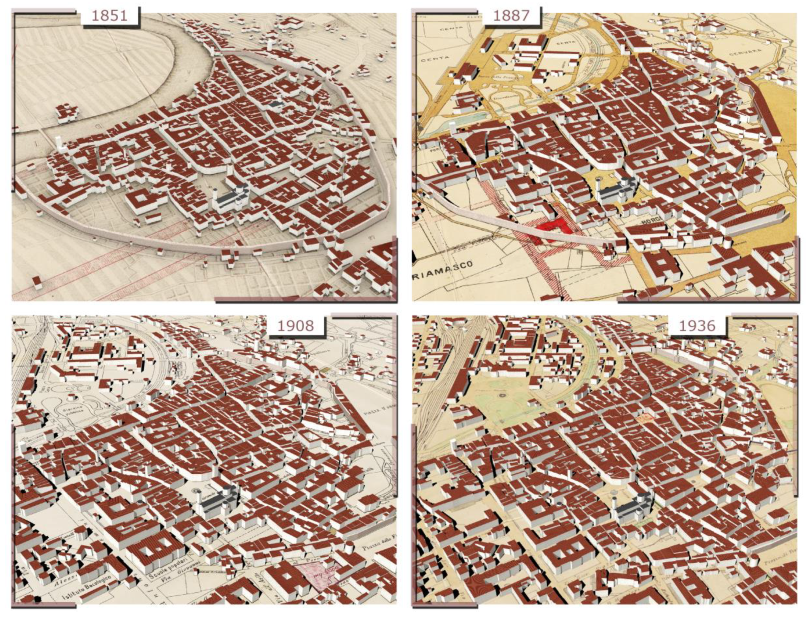
Article

4D Building Reconstruction with Machine Learning and Historical Maps

by
Elisa Mariarosaria Farella
1,
Emre Özdemir
1,2 and
Fabio Remondino
1,*
1
3D Optical Metrology (3DOM) Unit, Bruno Kessler Foundation (FBK), Via Sommarive 18, 38123 Trento, Italy
2
Skolkovo Institute of Technology (Skoltech), Bolshoy Boulevard 30, 121205 Moscow, Russia
*
Author to whom correspondence should be addressed.
Appl. Sci. 2021, 11(4), 1445; https://doi.org/10.3390/app11041445
Submission received: 2 January 2021 / Revised: 28 January 2021 / Accepted: 30 January 2021 / Published: 5 February 2021
(This article belongs to the Special Issue Analyses in Geomatics: Processing Spatial Data on History and Today)

Abstract

:
The increasing importance of three-dimensional (3D) city modelling is linked to these data’s different applications and advantages in many domains. Images and Light Detection and Ranging (LiDAR) data availability are now an evident and unavoidable prerequisite, not always verified for past scenarios. Indeed, historical maps are often the only source of information when dealing with historical scenarios or multi-temporal (4D) digital representations. The paper presents a methodology to derive 4D building models in the level of detail 1 (LoD1), inferring missing height information through machine learning techniques. The aim is to realise 4D LoD1 buildings for geospatial analyses and visualisation, valorising historical data, and urban studies. Several machine learning regression techniques are analysed and employed for deriving missing height data from digitised multi-temporal maps. The implemented method relies on geometric, neighbours, and categorical attributes for height prediction. Derived elevation data are then used for 4D building reconstructions, offering multi-temporal versions of the considered urban scenarios. Various evaluation metrics are also presented for tackling the common issue of lack of ground-truth information within historical data.

Graphical Abstract

1. Introduction

Historical maps are the most powerful source of information for understanding urban phenomena and changes that contributed to defining our cities’ actual shape. The growth and transformation of the urban patterns and landscapes can be analysed through these differently accurate, symbolised, and generalised representations of reality. Historical maps represent a graphically coded reduction of the three-dimensional (3D) world in the 2D space, which summarises the urban environment’s main features. The cities’ growth and changes—conditioned by preferred directions of expansion, natural constraints, and particular historical events—are impressed in these documents with several informative levels. Nevertheless, the 2D space-reduction of the maps entails an unavoidable loss of information, and particularly on the height of the built and natural environment.
With the advent of digital technologies, a more realistic and complete representation of the world has become possible in its three and four dimensions (3D/4D). Several geomatic and modelling techniques have been developed in the last years to generate 3D/4D city models, derived with different levels of automation and input data [1,2,3,4]. 3D/4D models can be digital copies of our cities when enriched with textural information or semantically enhanced when the geometry is linked to other attributes. Depending on their nature, they can be used for visualisation, simulations, geospatial analyses, planning activities, and many other applications [5]. The undisputable advantage offered by the three dimensions is the broader comprehension of the built spaces and relations in the urban pattern, as well as their interaction with the natural elements. Modelling in 3D multi-temporal versions of the same city (4D) can broaden how these relations and interactions are changed over time. Multi-temporal analyses and modelling of urban environments is typically performed using image or Light Detection and Ranging (LiDAR) data, deriving building height information from these data [6]. On the other hand, when only building footprints digitised from historical maps are available, the main issue is to derive the missing height information.

Aims and Innovative Aspects

This work aims to explore existing machine learning solutions for inferring building heights from historical maps. Multi-temporal versions (4D) of the same city are generated with predicted height values, expanding the space information essential for more comprehensive geospatial analyses and 3D modelling applications. This work is part of the TOTEM project (4D Trento Time Machine) (https://totem.fbk.eu/), focused on the development of ICT (Information and Communications Technology) and AI (Artificial Intelligence) solutions for the valorisation of historical data (maps and photos) preserved in the archives of Trento (Italy).
The developed methodology was firstly tested on four different historical maps of Trento (1851, 1887, 1908, and 1936). These maps (Section 3.1) depict many changes of the urban structure in the last 150 years, which involved both the historical city centre and the area outside the medieval defensive walls of Trento. The historical maps were georeferenced and building block shapes (“footprints”), including their partitioning, manually digitised in a GIS environment. A set of diverse polygons was thus generated and several attributes describing geometrical and neighbourhood features were computed for each digitised polygon (Section 4.1). Finally, machine learning algorithms were tested for predicting the block heights, using actual height values (derived from modern topographic data) as training data. The method has been verified (Section 4.4) adopting common machine learning quality metrics, examining in-depth the prediction performance on buildings still existing and with the same shape, or not existing anymore but documented in the historical photo. The replicability of the proposed methodology was also tested on the historic city centre of Bologna, Italy (Section 3.2).
The innovative aspects of the work are:
-
evaluation of multiple regressors to infer building heights from historical maps;
-
introduction of the geometric, neighbourhood, and categorical features usable when only digitised building footprints are available;
-
testing and evaluation of the proposed method on two different locations and multi-temporal historical maps; and
-
the realisation of 4D level of detail 1 (LoD1) building models for the geo-visualisation enhancement, creating a 4D cadastre, and spatial analysis purposes (e.g., volumetric density studies.

2. Related Works

3D city models are simplified digital replicas of the urban environments, mainly defined by the building blocks’ geometry, mutual relations, and the interaction with natural elements. 3D city modelling is a vast research area, centred on developing solutions to create models with several techniques, source data, and automation levels [7,8,9]. The application fields have extraordinarily increased in the last decades, bringing significant advantages in many domains (e.g., urban planning, crises and risks management, simulation studies) [10,11,12]. 3D city models are generally obtained from 3D surveyed reality-based data [13,14], employing SAR (Synthetic-Aperture Radar) techniques [15], extruding 2D building footprints [16], through procedural modelling [17], or volunteered geoinformation [18]. Elevation data are mostly derived from LiDAR airborne scanning or image-based procedures and are differently used for modelling purposes. Based on the available source data, employed approach, and the field of application, buildings can be represented with five levels of detail (LoD) [19] and stored with well-defined standards, such as CityGML [20,21] or CityJSON [22]. For visualisation and simple data analyses, the LoD1 (i.e., prismatic block with flat roofs) is sufficient and preferred. According to the available elevation data, the simplest and most common approach for generating LoD1 models is the extrusion of building footprints, generally considering the median or maximum height value [23,24]. When elevation data are missing, a rough building height estimation can be performed with other methods, e.g., counting the number of storeys, considering local regulations and related construction restrictions, or measuring the shadows’ length in imagery data [25,26,27,28]. The derived height values’ quality is rarely verified and out of scope in many applications with these approaches.
AI-based procedures were recently used to infer buildings’ features and characteristics. Machine and deep learning methods were increasingly employed for predicting 3D urban geometries and semantics [29,30,31,32], for energy performances [33,34,35], for models generalisation [36], or to infer some missing information, such as buildings’ age [37,38,39,40] and height [28,41,42,43,44]. Prediction algorithms are generally trained using satellite or aerial images [43,44], LiDAR data [37,42], or 2D data (such as photographs, maps, footprints, and attributes) available from historical archives, cadastre datasets, or volunteered geographic information databases [28,38,39,45].
For the 3D reconstruction of historical urban scenarios, buildings’ footprints and some neighbours or categorical features are the only information usable for the prediction. In [28] and [46], buildings’ heights are inferred exploiting some machine learning techniques, relying on cadastral and statistical data, as well as some geometrical information extracted from the footprints. We hereafter present a similar approach, based only on geometric, neighbour, and categorical features computable from the digitised historical buildings. With respect to other methods, the proposed approach does not include the number of storeys [28] (not always available and which could significantly vary in each regional contexts), and it only relies only on a set of features (“predictors”—Section 4.2) derived from the available building footprints, combined with data augmentation methods to derive accurate results over multiple years and locations.

3. Data and Case Studies

3.1. Trento (Italy) Historic City Centre

As a part of the TOTEM project, maps from four different years (1851, 1887, 1908, and 1936—Figure 1) were employed for this study. Throughout these years, the more significant changes in the city’s structure have been related to (i) the alteration of the river’s course, which conditioned the urban sprawl of the city and (ii) the progressive demolition of most of the defensive medieval walls. These changes in the urban pattern and the expansion of man-made structures are visible throughout the maps, whereas building functions or planned urban interventions are differently coded.
While in the oldest map (the year 1851), the buildings’ aggregation in blocks and their relation with the cultivated areas are quite detailed, the 1887 map features a more draft representation of the urban landscape (Figure 1), with buildings aggregated in large footprints. In this case, only a few significant civil and religious buildings are sufficiently mapped, while other structures can be identified only by comparing historical data. The informative level of the last two maps (years 1908 and 1936) is instead suitable enough for highlighting the main features and transformation of the built urban environment (Table 1).
After the manual digitisation of building footprints and each historical map’s georeferencing, several attributes (predictors—Section 4.2) were computed. For training the predictive models, footprints and their respective height values derived from the actual topographic data (2016) were employed (Table 2). From this data set (Figure 2), some temporally inconsistent constructions, as recent and industrial structures, were removed to avoid erroneous predictions.
As reported in Section 5.1, two buildings’ classes proved to be an under-represented category in the training data, namely religious structures and civil towers. A data augmentation approach was therefore applied to reach a more balanced class representation and more accurate reconstructions of these few but relevant buildings, describing the city-skyline and aspect.

3.2. Bologna (Italy) Historic City Centre

As a further case study, the historic city centre of Bologna was considered. Two historical maps describing the city in 1884 and 1945 were selected and manually digitised in GIS Environment (Figure 3). In the older case, medieval defensive walls surrounding the city are still clearly visible, while in the 1945 map, damages of the Second World War and planned building reconstruction interventions are reported. Moreover, in this case, the two historical maps’ level of information is quite different. In the oldest representation (1884), few details on the building blocks partitioning are provided with respect to the more recent map (Table 3).
Some characteristics of the actual topographic data (Figure 4) used for training the regression models are reported in Table 4. Results of building heights prediction are presented in Section 5.3.

4. Methodology

This section introduces the tested regression methods for inferring buildings’ heights from digitised historical maps (Section 4.1). Predictors (Section 4.2), data augmentation (Section 4.3), and evaluation metrics (Section 4.4) are then presented. Heights values, predicted with some machine and deep learning techniques, are thus used for obtaining multi-temporal 3D models of the case studies in LoD1. The method is based on the construction of regression models (Figure 5), able to predict the values of a target variable based on some predictor variables.

4.1. Machine and Deep Learning for Regression Models

Within the machine and deep learning applications, the regression problem is a common task. Regression analysis is a predictive modelling technique that predicts numerical variables y, typically called target, based on one or multiple variables x (predictors) [47]. Thus, a regression model aims to build a mathematical equation that defines the target y as a function of the predictor x. Once the model is trained, it can use new predictor values to infer y. In this work, several and common regression models, mainly available in the scikit-learn library [48], were tested for inferring the building heights from a set of predictor variables (Section 4.2), in particular:
(a).
Ordinary Least Squares Linear regressor: this model minimises the residual sum of squares between the observed and target variables. It assumes a linear connection between outputs and predictor variables, and it is sensitive to random errors when variables are not independent [49].
(b).
Random Forest regressor: it is a supervised learning algorithm based on ensemble learning. Random Forest combines multiple decision trees (reducing the variance and overfitting) resulting in an averaged prediction of the individual classifiers. It also provides straightforward methods for the features’ importance analysis and selection [50].
(c).
CatBoost regressor: it uses gradient boosting on decision trees. The decision tree is used as a weak base learner, while gradient boosting iteratively fits a sequence of these trees [51].
(d).
Support Vector regressor with the Radius Basis Function (RBF) kernel: it produces a model depending only on a subset of the training data. The employed cost function ignores samples whose prediction is close to their target [52].
(e).
Multilayer Perceptron regressor: it is a neural network model where neurons are arranged in different layers, connected by differently weighted joints [53]. The model optimises the squared loss using, e.g., stochastic gradient descent.

4.2. Predictors

A predictor is a variable used to train a specific learning model to predict something. According to their informative level and reported details, historical maps are the only source for deriving information about building footprints and their spatial distribution in the past. Aside from the building’s shape, some blocks’ designated use is generally the only additional information obtained from these documents. Data on building heights can be exclusively derived comparing blocks still existing in the same shape, or, approximately, from available photos in the other cases. When data are only derived by historical maps, the selection of the predictors is conditioned by the lack of further cadastral information (e.g., the number of storeys) or aerial views. Therefore, geometric properties and position of the digitised blocks, as well as data from neighbourhood analyses, are the only features usable for the prediction. In this work, three different types of attributes were computed for each digitised building footprint and used as predictors for inferring building heights:
-
Geometric predictors:
(1).
Area: defined as the building footprint area;
(2).
Perimeter: defined as the footprint perimeter;
(3).
NPI: the normalised perimeter index, an indicator of the polygon shape complexity. It is computed as the ratio of the perimeter of the equal-area circle and the perimeter of the shape (1):
N P I = 2 π A p
(4).
Vertices: the number of vertices of a digitised polygon (Figure 6a);
(5).
Length MBR: the length of the minimum bounding rectangle (MBR) of a footprint;
(6).
Width MBR: the width of the minimum bounding rectangle (MBR) of a footprint;
(7).
Area MBR: the area of the minimum bounding rectangle (MBR) of a footprint;
(8).
Ratio: the ratio between the area of a footprint and the area of the corresponding minimum boundary rectangle (MBR).
-
Neighbourhood predictors:
(9).
Neighbours: defined as the number of adjacent polygons;
(10).
Distance: the distance of a polygon’s centroid from the nearest centroid (Figure 6b);
(11).
Density: the kernel density values (Figure 6c), considering four different estimation radii (50 m, 100 m, 150 m, 200 m), defined as (2):
D e n s i t y = 1 ( r a d i u s ) 2 i = 1 n [   3   π p o p   ( 1 ( d i s t r a d i u s 2 ) 2 ) ]
where i = 1…,n, are the input points, pop is the population field of the point i, and dist is the distance between point i and the (x, y) location.
-
Positional and categorical predictors:
(12).
Position (X, Y): the planar position of each polygon centroid within the map;
(13).
Group: the aggregation of polygons in building blocks (Figure 6d). A “group” value is assigned to each polygon belonging to the same building block, while isolated buildings are grouped;
(14).
Class: defines a building of specific historical value, such as churches, palaces, castle, and tower;
(15).
Function: defines the civil or religious function of the buildings. In our cases, civil buildings were also grouped considering their approximative period of construction, derived by comparing multi-temporal historical maps;
(16).
Towers: includes a shape-based classification of the civil and religious towers, i.e., circular, rectangular, or octagonal shape. In our cases, we noticed that towers with similar shapes featured similar heights.
The computed predictor values, especially for the geometric and neighbour attributes, are strongly conditioned by the historical maps’ level of detail and the consequent digitisation (Figure 1). Based on the quality of the building footprints (i.e., depicting a single building or a group), attribute values can significantly vary. Their combination with further attributes has been introduced to support the predictions, especially when the digitised maps suffer from a poor representation of man-made structures.

4.3. Data Augmentation

Data augmentation is a technique used to increase the quantity of data and is based on generating either altered versions of the existing data or artificial data. It is most commonly used for dealing with overfitting as well as creating more sample data, e.g., in deep learning processes [54,55,56,57]. In data augmentation, sample sets are expanded, generating synthetic data through any geometric or colorimetric transformation [58,59].
When dealing with urban data and modelling applications, some building classes are commonly under-represented. In historical centres, this condition occurs with two main categories of buildings, i.e., religious structures and civil towers, both strongly typifying the shape and skyline of the cities. In similar situations, the learning process could be affected by under-represented classes. Hence, re-sampling classes distribution and randomly adding geometrically modified copies of the weakly represented structures could be necessary to process more balanced datasets and improve the model performances.
In this work, augmented buildings are positioned outside the city without overlapping existing ones. The feature extraction is then handled together with all buildings. The augmentation is based on the existing buildings’ data, with modifications on their geometrical properties, including dimensions and orientation. The augmented data is used for only training.

4.4. Heights Prediction Metrics

Three different approaches are proposed for evaluating the quality of the inferred building heights.

4.4.1. Evaluation of the RMSE, MAE, and R2 on Randomly Split Training and Test Data

In machine learning applications, the prediction quality considers how well a model performs on data not used when fitting the model. Therefore, data are commonly split into training and test datasets (typically 70% and 30%, respectively), where the training is used to estimate parameters of the predictive method and the test dataset for evaluating its accuracy. When data augmentation (Section 4.3) is used, those data falling in the test dataset are moved to the training dataset. Most used metrics for evaluating the quality of the models are the root mean square error (RMSE) (3), the mean absolute error (MAE) (4), and R2 (coefficient of determination) (5). They are respectively defined as:
R M S E = 1 n j = 1 n ( y j y ^ j ) 2
M A E = 1 n j = 1 n | y j y ^ j |
R 2 ( y ,   y ^ ) = 1 i = 1 n ( y i y ^ i ) 2 i = 1 n ( y i y ¯ ) 2
Median of the height differences (ground truth vs. predicted) and standard deviation are also used and reported as evaluation metrics.
A more in-depth control of the machine learning prediction quality can be performed adopting—as a test set—a small subset of still existing buildings having the same shape and being present on different historical maps.

4.4.2. Single-View Metrology from Historical Images

Assessing the quality of the prediction of disappeared buildings is more complicated. If historical images are available, single-view metrology [60,61] and fundamental invariants of projective geometry [62] can be used. An essential property of projective geometry is that some measures are invariant to projective transformations. The cross-ratio invariant and image vanishing points can be used for deriving distance measurements from a single image. Knowing one reference distance (H), the method (Figure 7) implies that the height of the camera (HC) and any other distance (HU) between two planes perpendicular to the reference direction (v3) can be derived. Two points B and T, lying on two planes P and P’ perpendicular to the reference direction v3, are represented in image space by points b and t lying on the two planes defined by the two vanishing points v1 and v2. The image point lies at the intersection of the line joining the corresponding points C (the camera centre) and C’ with the vanishing line lv1v2. The point C lies on a plane at a distance HC from the reference plane P. Under this configuration, the image points b, t, c, and v3 are aligned along the vertical reference direction, and therefore they define a cross-ratio. The ratio also holds in object space with points B, T, C’, and v3. Therefore, we can derive (6):
H H C = 1 d   ( t , c ) d ( b , v 3 ) d   ( b , c ) d ( t , v 3 )
where d(a, b) is the Euclidean distance between points a and b, measured in image space. Therefore, if we know a vertical reference height in the scene (e.g., a building, a person), we can derive a building’s height and use this information to evaluate a prediction.

4.5. Accuracy Aims

The two considered urban scenarios present similar volumetric characteristics, peculiar to the construction techniques of northern Italy. The predominance of buildings with numerous pitched roofs and variable slopes makes these test cases quite tricky. For the variety of roof examples and the peculiarities of such stratified urban contexts, a mean absolute error (MAE) of about 2 m was considered a satisfying accuracy target for this work, in accordance with results presented in the literature [28,46]. This accuracy target considers that higher error values can be expected with a random test set since many ground-truth buildings could be temporally inconsistent or changed over time. More accurate results are contemplated for a subset of buildings, unaltered in the considered time-periods.

5. Results

In this section, regression model performances and results of the predictions on historical data are presented (Section 5.1). A more comprehensive investigation is reported for the Trento case study (Section 5.2). The second dataset, Bologna, shows the replicability of the proposed method (Section 5.3).

5.1. Regressors Evaluation

The actual topographic databases of both case studies (Section 3) were used, with the computed predictors (Section 4.2), to evaluate the performances of the selected regressor methods (Section 4.1). Data were randomly split into training and test sets and metrics computed. Table 5 and Table 6 show the performances of the different height predictions over Trento and Bologna, respectively.
In our tests, the Random Forest (RF) regressor proved to outperform the other algorithms with respect to all chosen metrics (Section 4.4).
Although RF metrics were quite close to our target accuracy (MAE ~ 2 m), an authentic look at the predicted heights of specific buildings show the presence of gross errors in particular for the building classes with fewer samples, i.e., religious buildings and towers (Figure 8).
A non-uniform composition of data is evident in terms of distribution, as shown in Figure 9 left and Table 7. Therefore, a data augmentation approach was applied for churches and towers to achieve a more balanced representation of all classes (Table 8, Figure 9 right).
The evaluation of the chosen regressor method was performed again on the new “augmented” dataset: results (Table 9 and Table 10) show slight accuracy improvements and still prove that RF performs better than the others.
Aside from the slight improvement of the evaluation metrics, the adopted data augmentation approach’s effectiveness is proven by reduced gross errors in the under-represented classes and the more precise height predictions all over the city (Figure 10).

5.2. Inferring Building Heights from a Historical Map—Trento Case Study

The building footprints digitised in the four historical maps (1851, 1887, 1908, and 1936) of Trento and their predictors (Section 4.2) were used to infer building heights using the two outperforming predictor methods: Random Forest and Catboost. The actual topographic database was used to learn heights, although some modern buildings were removed beforehand from the input data to limit gross errors. Evaluation metrics to check predicted heights in the historical maps were computed on a smaller test set, including only some buildings still existing, having the same shape and recognisable in the different maps. Table 11 and Table 12 show the height difference error calculated in this case, presenting the Random Forest and Catboost results, which demonstrated to be the best performing algorithms (Section 5.1). Again, the Random Forest confirmed to outperform the other algorithms.
As a further check of the prediction’s quality, single-view metrology (Section 4.4.2) was applied to derive some ground-truth heights for disappeared buildings. Vanishing lines and cross-ratio invariants were used with some historical photos where a known height was measurable (Figure 11). Table 13 summarises the evaluation results adopting the presented procedure.
Visual results of the 4D LoD1 reconstruction of Trento are presented in Figure 12 and Figure 13. An example of texture mapping with a historical photo is shown in Figure 14.

5.3. Inferring Building Heights from a Historical Map—Bologna Case Study

The implemented method was also tested on two historical versions of the Bologna city centre (1884 and 1945). Among the transformations of the city in this time frame, the almost complete destruction of the medieval defensive walls and the heavy damages of war bombardments are the most relevant.
Starting from the city’s actual topographic database and following the regressors evaluation (Section 5.1), Random Forest and Catboost methods were used to predict building heights in the historical maps. The predicted heights evaluation was performed, considering only some unchanged buildings as a test set (Table 14 and Table 15). Figure 15 presents some general and detailed views of the 3D buildings reconstruction for the Bologna city centre.

6. Discussion

The quality performance of several regressors for predicting height values from historical data was presented. Several evaluation approaches were proposed for tackling the issue of a lack of ground-truth information with historical data. The evaluation metrics proved that the Random Forest regressor inferred better building heights with regard to other algorithms.
Comparing the prediction results with the Random Forest algorithm in the historical datasets (Table 11 and Table 14), a general worsening of the metrics can be noticed when the polygon’s area is much different from the training data (Table 1 and Table 3). Therefore, the prediction quality is conditioned by the informative level of the historical maps and size of digitised polygons.
The inferring methodology relies on some twenty predictors (Section 4.2). As typical in a machine learning application, a recursive feature elimination (RFE) approach can be employed to select and reduce the predictors. This technique helps remove irrelevant predictors, selecting only the most relevant ones and speeds up the overall prediction procedure. Figure 16 reports the predictors’ importance for the Trento dataset. Some categorical features are more significant than other attributes. Therefore, an RFE approach was applied to optimise the algorithm’s performance and reduce the number of predictors (Figure 17). Results and comparisons for both datasets are presented in Table 16 and Table 17.
Aside from no significant changes in the evaluation metrics, a general worsening in the predicted building heights’ quality was verified by visually checking the results obtained after an RFE approach. Therefore, for the considered datasets, the RFE approach proved to be ineffective, and the different contributions of all predictors (Section 4.2) were shown to be relevant.
The implemented method, although reliable and feasible, still presents some issues to be tackled:
(a).
data preparation (i.e., the digitisation of historical maps) is demanding and time-consuming;
(b).
differences in the input data (i.e., different informative levels among the training data and the historical datasets) can affect the quality of the prediction;
(c).
the results can be influenced by the accuracy of the georeferenced maps, considering that positional attributes are included among the predictors; and
(d).
the method was tested on similar urban scenarios and using respective actual data as training. The applicability in different regional contexts and the prediction’s quality employing other cities’ training data need further investigations.
About the latter issue, some preliminary tests were conducted to verify if, in similar built environments, the procedure can return satisfactory results using different cities’ training data. The Random Forest performances’ evaluation are presented in Table 18 where a training using Trento’s data is used to predict heights of Bologna footprints, and vice-versa (removing the positional attributes). Although quality metrics are relatively consistent (or even better) with the results reported in Table 5 and Table 6, a visual check (Figure 18) highlights a general wrong prediction of civil towers and religious buildings. Furthermore, significant errors can be noticed in sparse and isolated buildings outside the city centre, due to the implemented data augmentation technique (Section 4.3). Without positional attributes, the presence of an increased number of sparse polygons (towers and religious buildings) in the training data, proved to negatively condition the learning method.
The quality of the prediction was further verified, removing augmented data with inverted trainings. Metrics and some visual results are presented in Table 19 and Figure 19.
The accuracy results show an opposite trend in the two datasets. Visual outcomes highlight an acceptable prediction for polygons inserted in building blocks and a slight improvement for isolated constructions. These preliminary experiments are promising for the generalisation of the method and its applicability in several contexts.

7. Conclusions

Multi-temporal (4D) versions of the same urban area are of beneficial interest for landscape and urban analyses. This work presented a methodology for the digital reconstruction of buildings in 4D with machine learning algorithms and historical data.
From digitised historical maps and information of the actual city situations, different regression algorithms were compared and employed for inferring missing building heights, using this information for the multi-temporal 3D reconstruction of two urban city centres.
The reliability of the proposed approach was verified, testing the method on different datasets and epochs. Multiple quality evaluation methods were also proposed to tackle the issue of missing ground-truth data. The achieved results proved to be consistent with our accuracy targets and the complexity of such historical urban contexts. The implemented method is flexible and extendable, relying mainly on geometric and neighbour characteristics derivable from the datasets and adaptable categorical data.
In future investigations, the method will be extended to tackle the several issues presented in the previous section, exploring:
(a).
automatic methods and deep learning techniques for replacing the time-consuming digitisation procedure of historical maps;
(b).
the use of specific training data (e.g., prepared at a building-block level rather than using detailed cadastral maps) for historical datasets suffering from a low informative level;
(c).
the prediction response assigning a lower weight to positional attributes, for avoiding possible mismatches related to different-scale maps and georeferencing issues; and
(d).
the possible generalisation of the method, expanding the training set with data representative of different regional contexts, and applying the trained model in actual scenarios where no elevation data are available (e.g., remote areas).

Author Contributions

The article presents a research contribution that involved authors in equal measure. F.R. supervised the overall work and reviewed the entire paper, writing the introduction, aim, and conclusions of the paper; E.M.F. dealt with the state of the art, methodology, data processing, and results. E.Ö. was mainly involved in the development of the regressor analysis, methodology development, and paper revision. All authors have read and agreed to the published version of the manuscript.

Funding

The presented work belongs to the TOTEM project activities which are financially supported by Fondazione CARITRO (https://www.fondazionecaritro.it/).

Institutional Review Board Statement

Not applicable.

Informed Consent Statement

Not applicable.

Data Availability Statement

Not applicable.

Acknowledgments

Authors are thankful to the Cadastral office and Superintendence for Cultural Heritage of the Autonomous Province of Trento, Fondazione Museo Storico del Trentino, Archivio Fotografico Storico, and Municipality of Trento.

Conflicts of Interest

The authors declare no conflict of interest.

References

  1. Döllner, J.; Kolbe, T.H.; Liecke, F.; Sgouros, T.; Teichmann, K. The virtual 3D city model of Berlin: Managing, integrating, and communicating complex urban information. In Proceedings of the 25th Urban Data Management Symposium, Aalborg, Denmark, 15–17 May 2006; pp. 15–17. [Google Scholar]
  2. Kersten, T.P.; Keller, F.; Sänger, J.; Schiewe, J. Automated Generation of an Historic 4D City Model of Hamburg and Its Visualisation with the GE Engine; Springer: Berlin/Heidelberg, Germany, 2012; Volume 7616. [Google Scholar]
  3. Singh, S.; Jain, K.; Mandla, V.R. Virtual 3D city modeling: Techniques and applications. Int. Arch. Photogramm. Remote Sens. Spat. Inf. Sci. 2013, 73–91. [Google Scholar] [CrossRef] [Green Version]
  4. Kocaman, S.; Akca, D.; Poli, D.; Remondino, F. 3D/4D City Modelling—From Sensors to Applications; Whittles Publishing: Scotland, UK, 2020; ISBN 978-184995-475-4. [Google Scholar]
  5. Biljecki, F.; Stoter, J.; Ledoux, H.; Zlatanova, S.; Çöltekin, A. Applications of 3D city models: State of the art review. ISPRS Int. J. Geo-Inf. 2015, 4, 2842–2889. [Google Scholar] [CrossRef] [Green Version]
  6. Nocerino, E.; Menna, F.; Remondino, F. Multi-temporal analysis of landscapes and urban areas. Int. Arch. Photogramm. Remote Sens. Spat. Inf. Sci. 2012, 39, B4. [Google Scholar] [CrossRef] [Green Version]
  7. Haala, N.; Kada, M. An update on automatic 3D building reconstruction. ISPRS J. Photogramm. Remote Sens. 2010, 65, 570–580. [Google Scholar] [CrossRef]
  8. Haala, N.; Rothermel, M.; Cavegn, S. Extracting 3D urban models from oblique aerial images. In Proceedings of the 2015 Joint Urban Remote Sensing Event (JURSE), Lausanne, Switzerland, 30 March—1 April 2015; pp. 1–4. [Google Scholar]
  9. Buyukdemircioglu, M.; Kocaman, S.; Isikdag, U. Semi-automatic 3D city model generation from large-format aerial images. ISPRS Int. J. Geo-Inf. 2018, 7, 339. [Google Scholar] [CrossRef] [Green Version]
  10. Chen, R. The development of 3D city model and its applications in urban planning. In Proceedings of the 2011 19th International Conference on Geoinformatics, Shanghai, China, 24–26 June 2011; pp. 1–5. [Google Scholar]
  11. Ghassoun, Y.; Löwner, M.-O.; Weber, S. Exploring the benefits of 3D city models in the field of urban particles distribution modelling—A comparison of model results. In 3D Geoinformation Science; Springer: Berlin/Heidelberg, Germany, 2015; pp. 193–205. [Google Scholar]
  12. Willenborg, B.; Sindram, M.; Kolbe, T.H. Applications of 3D city models for a better understanding of the built environment. In Trends in Spatial Analysis and Modelling; Springer: Berlin/Heidelberg, Germany, 2018; pp. 167–191. [Google Scholar]
  13. Tomljenovic, I.; Höfle, B.; Tiede, D.; Blaschke, T. Building extraction from airborne laser scanning data: An analysis of the state of the art. Remote Sens. 2015, 7, 3826–3862. [Google Scholar] [CrossRef] [Green Version]
  14. Yalcin, G.; Selcuk, O. 3D city modelling with Oblique Photogrammetry Method. Procedia Technol. 2015, 19, 424–431. [Google Scholar] [CrossRef] [Green Version]
  15. Ali, I.; Khan, A.A.; Qureshi, S.; Umar, M.; Haase, D. 3D Geoinformation Science, Lecture Notes in Geoinformation and Cartographyitle; Breunig, M., Al-Doori, M., Butwilowski, E., Kuper, P.V., Benner, J., Haefele, K.H., Eds.; Springer: Berlin/Heidelberg, Germany, 2015. [Google Scholar]
  16. Arroyo Ohori, K.; Ledoux, H.; Stoter, J. A dimension-independent extrusion algorithm using generalisedgeneralised maps. Int. J. Geogr. Inf. Sci. 2015, 29, 1166–1186. [Google Scholar] [CrossRef]
  17. Smelik, R.M.; Tutenel, T.; Bidarra, R.; Benes, B. A survey on procedural modelling for virtual worlds. Comput. Graph. Forum 2014, 33, 31–50. [Google Scholar] [CrossRef]
  18. Goetz, M.; Zipf, A. Towards defining a framework for the automatic derivation of 3D CityGML models from volunteered geographic information. Int. J. 3D Inf. Model. 2012, 1, 1–16. [Google Scholar] [CrossRef]
  19. Biljecki, F.; Ledoux, H.; Stoter, J. An improved LOD specification for 3D building models. Comput. Environ. Urban Syst. 2016, 59, 25–37. [Google Scholar] [CrossRef] [Green Version]
  20. Gröger, G.; Plümer, L. CityGML—Interoperable semantic 3D city models. ISPRS J. Photogramm. Remote Sens. 2012, 71, 12–33. [Google Scholar] [CrossRef]
  21. Gröger, G.; Kolbe, T.H.; Nagel, C.; Häfele, K.H. OGC City Geography Markup Language (CityGML) Encoding Standard; Version 2.0.0, OGC 08-007r2; Open Geospatial Consortium: Wayland, MA, USA, 2012. [Google Scholar]
  22. Ledoux, H.; Ohori, K.A.; Kumar, K.; Dukai, B.; Labetski, A.; Vitalis, S. CityJSON: A compact and easy-to-use encoding of the CityGML data model. Open Geospat. Data Softw. Stand. 2019, 4, 4. [Google Scholar] [CrossRef]
  23. Ledoux, H.; Meijers, M. Topologically consistent 3D city models obtained by extrusion. Int. J. Geogr. Inf. Sci. 2011, 25, 557–574. [Google Scholar] [CrossRef] [Green Version]
  24. Shi, Y.; He, B. Creating Topologically Consistent 3D City Models of LOD+ with Extrusion. In Proceedings of the International Conference on Computer and Computing Technologies in Agriculture, Zhangjiajie, China, 19–21 October 2012; pp. 203–210. [Google Scholar]
  25. Fan, H.; Zipf, A. Modelling the world in 3D from VGI/Crowdsourced data. In European Handbook of Crowdsourced Geographic Information; Ubiquity Press: London, UK, 2016; pp. 435–466. [Google Scholar]
  26. Brasebin, M.; Perret, J.; Mustière, S.; Weber, C. A generic model to exploit urban regulation knowledge. ISPRS Int. J. Geo-Inf. 2016, 5, 14. [Google Scholar] [CrossRef] [Green Version]
  27. Peeters, A. A GIS-based method for modeling urban-climate parameters using automated recognition of shadows cast by buildings. Comput. Environ. Urban Syst. 2016, 59, 107–115. [Google Scholar] [CrossRef]
  28. Biljecki, F.; Ledoux, H.; Stoter, J. Generating 3D city models without elevation data. Comput. Environ. Urban Syst. 2017, 64, 1–18. [Google Scholar] [CrossRef] [Green Version]
  29. Rook, M.; Biljecki, F.; Diakité, A.A. Towards Automatic Semantic Labelling of 3D City Models. ISPRS Ann. Photogramm. Remote Sens. Spat. Inf. Sci. 2016, 4. [Google Scholar] [CrossRef]
  30. Wichmann, A.; Agoub, A.; Kada, M. Roofn3D: Deep Learning Training Data for 3D Building Reconstruction. Int. Arch. Photogramm. Remote Sens. Spat. Inf. Sci. 2018, 42, 1191–1198. [Google Scholar] [CrossRef] [Green Version]
  31. Agoub, A.; Schmidt, V.; Kada, M. Generating 3D City Models Based on the Semantic Segmentation of Lidar Data Using Convolutional Neural Networks. ISPRS Ann. Photogramm. Remote Sens. Spat. Inf. Sci. 2019, 4, 3–10. [Google Scholar] [CrossRef] [Green Version]
  32. Tripodi, S.; Duan, L.; Trastour, F.; Poujad, V.; Laurore, L.; Tarabalka, Y. Deep learning-based extraction of building contours for large-scale 3D urban reconstruction. In Proceedings of the Image and Signal Processing for Remote Sensing XXV, Strasbourg, France, 9–11 September 2019; Volume 11155, p. 111550O. [Google Scholar]
  33. Lee, S.; Jung, S.; Lee, J. Prediction model based on an artificial neural network for user-based building energy consumption in South Korea. Energies 2019, 12, 608. [Google Scholar] [CrossRef] [Green Version]
  34. Benavente-Peces, C.; Ibadah, N. Buildings Energy Efficiency Analysis and Classification Using Various Machine Learning Technique Classifiers. Energies 2020, 13, 3497. [Google Scholar] [CrossRef]
  35. Mohammadiziazi, R.; Bilec, M.M. Application of machine learning for predicting building energy use at different temporal and spatial resolution under climate change in USA. Buildings 2020, 10, 139. [Google Scholar] [CrossRef]
  36. Wu, Y.; Filippovska, Y.; Schmidt, V.; Kada, M. Application of Deep Learning for 3D building generalization. In Proceedings of the 29th International Cartographic Conference (ICC 2019), Tokyo, Japan, 15–20 July 2019. [Google Scholar]
  37. Tooke, T.R.; Coops, N.C.; Webster, J. Predicting building ages from LiDAR data with random forests for building energy modeling. Energy Build. 2014, 68, 603–610. [Google Scholar] [CrossRef]
  38. Biljecki, F.; Sindram, M. Estimating building age with 3D GIS. In Proceedings of the 12th International 3D GeoInfo Conference 2017, Melbourne, Australia, 26–27 October 2017; pp. 17–24. [Google Scholar]
  39. Zeppelzauer, M.; Despotovic, M.; Sakeena, M.; Koch, D.; Döller, M. Automatic prediction of building age from photographs. In Proceedings of the 2018 ACM on International Conference on Multimedia Retrieval, Yokohama, Japan, 11–14 June 2018; pp. 126–134. [Google Scholar]
  40. Mahajan, N.; Patil, D.; Kotkar, A.; Wasnik, K. Prediction of Building Structure Age Using Machine Learning. Int. J. Adv. Res. Ideas Innov. Technol. 2019, 5, 232–234. [Google Scholar]
  41. Mou, L.; Zhu, X.X. IM2HEIGHT: Height estimation from single monocular imagery via fully residual convolutional-deconvolutional network. arXiv 2018, arXiv:1802.10249. [Google Scholar]
  42. Park, Y.; Guldmann, J.-M. Creating 3D city models with building footprints and LIDAR point cloud classification: A machine learning approach. Comput. Environ. Urban Syst. 2019, 75, 76–89. [Google Scholar] [CrossRef]
  43. Liu, C.-J.; Krylov, V.A.; Kane, P.; Kavanagh, G.; Dahyot, R. IM2ELEVATION: Building Height Estimation from Single-View Aerial Imagery. Remote Sens. 2020, 12, 2719. [Google Scholar] [CrossRef]
  44. Mahmud, J.; Price, T.; Bapat, A.; Frahm, J.-M. Boundary-Aware 3D Building Reconstruction from a Single Overhead Image. In Proceedings of the IEEE/CVF Conference on Computer Vision and Pattern Recognition, Seattle, WA, USA, 14–19 June 2020; pp. 441–451. [Google Scholar]
  45. Kapoor, A.; Larco, H.; Kiveris, R. Nostalgin: Extracting 3D City Models from Historical Image Data. In Proceedings of the 25th ACM SIGKDD International Conference on Knowledge Discovery & Data Mining, Anchorage, AK, USA, 4–8 August 2019; pp. 2565–2575. [Google Scholar]
  46. Anh, P.; Thanh, N.T.N.; Vu, C.T.; Ha, N.V.; Hung, B.Q. Preliminary Result of 3D City Modelling for Hanoi, Vietnam. In Proceedings of the 2018 5th NAFOSTED Conference on Information and Computer Science (NICS), Ho Chi Minh City, Vietnam, 23–24 November 2018; pp. 294–299. [Google Scholar]
  47. Choi, R.Y.; Coyner, A.S.; Kalpathy-Cramer, J.; Chiang, M.F.; Campbell, J.P. Introduction to machine learning, neural networks, and deep learning. Transl. Vis. Sci. Technol. 2020, 9, 14. [Google Scholar]
  48. Pedregosa, F.; Varoquaux, G.; Gramfort, A.; Michel, V.; Thirion, B.; Grisel, O.; Blondel, M.; Prettenhofer, P.; Weiss, R.; Dubourg, V.; et al. Scikit-learn: Machine learning in Python. J. Mach. Learn. Res. 2011, 12, 2825–2830. [Google Scholar]
  49. Rong, S.; Bao-wen, Z. The research of regression model in machine learning field. In Proceedings of the MATEC Web of Conferences 2018 6th International Forum on Industrial Design (IFID 2018), Luoyang, China, 18–20 May 2018; Volume 176, p. 1033. [Google Scholar]
  50. Breiman, L. Random Forests. Mach. Learn. 2001, 45, 5–32. [Google Scholar] [CrossRef] [Green Version]
  51. Hancock, J.T.; Khoshgoftaar, T.M. CatBoost for big data: An interdisciplinary review. J. Big Data 2020, 7, 1–45. [Google Scholar] [CrossRef]
  52. Awad, M.; Khanna, R. Support vector regression. In Efficient Learning Machines; Springer: Berlin/Heidelberg, Germany, 2015; pp. 67–80. [Google Scholar]
  53. Murtagh, F. Multilayer perceptrons for classification and regression. Neurocomputing 1991, 2, 183–197. [Google Scholar] [CrossRef]
  54. Wong, S.C.; Gatt, A.; Stamatescu, V.; McDonnell, M.D. Understanding data augmentation for classification: When to warp? In Proceedings of the 2016 International Conference on Digital Image Computing: Techniques and Applications (DICTA), Gold Coast, Australia, 30 November–2 December 2016; pp. 1–6. [Google Scholar]
  55. Perez, L.; Wang, J. The effectiveness of data augmentation in image classification using deep learning. arXiv 2017, arXiv:1712.04621. [Google Scholar]
  56. Shorten, C.; Khoshgoftaar, T.M. A survey on image data augmentation for deep learning. J. Big Data 2019, 6, 60. [Google Scholar] [CrossRef]
  57. Zheng, Q.; Yang, M.; Tian, X.; Jiang, N.; Wang, D. A Full Stage Data Augmentation Method in Deep Convolutional Neural Network for Natural Image Classification. Discret. Dyn. Nat. Soc. 2020, 2020, 4706576. [Google Scholar] [CrossRef]
  58. Paschali, M.; Simson, W.; Roy, A.G.; Göbl, R.; Wachinger, C.; Navab, N. Manifold Exploring Data Augmentation with Geometric Transformations for Increased Performance and Robustness. In Proceedings of the International Conference on Information Processing in Medical Imaging, Hong Kong, China, 2–7 June 2019; pp. 517–529. [Google Scholar]
  59. Kim, E.K.; Lee, H.; Kim, J.Y.; Kim, S. Data Augmentation Method by Applying Color Perturbation of Inverse PSNR and Geometric Transformations for Object Recognition Based on Deep Learning. Appl. Sci. 2020, 10, 3755. [Google Scholar] [CrossRef]
  60. Criminisi, A.; Reid, I.; Zisserman, A. Single view geometry. Int. J. Comput. Vis. 2000, 40, 123–148. [Google Scholar] [CrossRef]
  61. Remondino, F. Recovering metric information from old monocular video sequences. In Proceedings of the 6th Conference on Optical 3D Measurement Techniques, Zürich, Switzerland, 22–25 September 2003. [Google Scholar]
  62. Semple, J.G.; Kneebone, G.T. Algebraic Projective Geometry; Oxford University Press: Oxford, UK, 1998. [Google Scholar]
Figure 1. The four digitised historical maps of Trento (1851, 1887, 1908, and 1936). Please note the different levels of detail of building footprints, e.g., between 1851 and 1887: in the latter case, footprints are bigger and include multiple buildings with regard to the other maps.
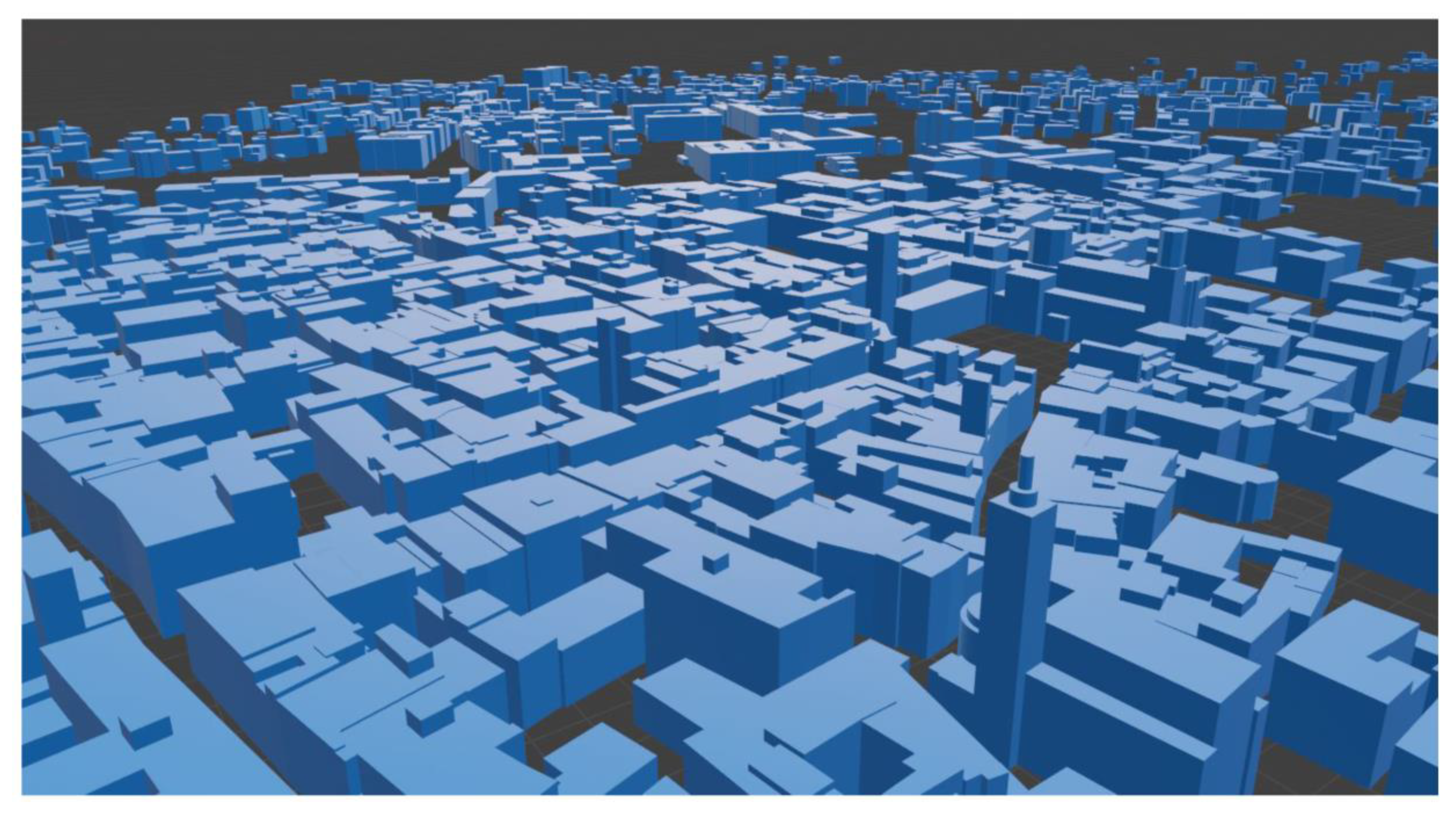
Applsci 11 01445 g001
Figure 2. A view of the level of detail 1 (LoD1) buildings in Trento generated from the actual (2016) topographic data available as open data. Height values are referred to as the mean level of the pitched roofs.
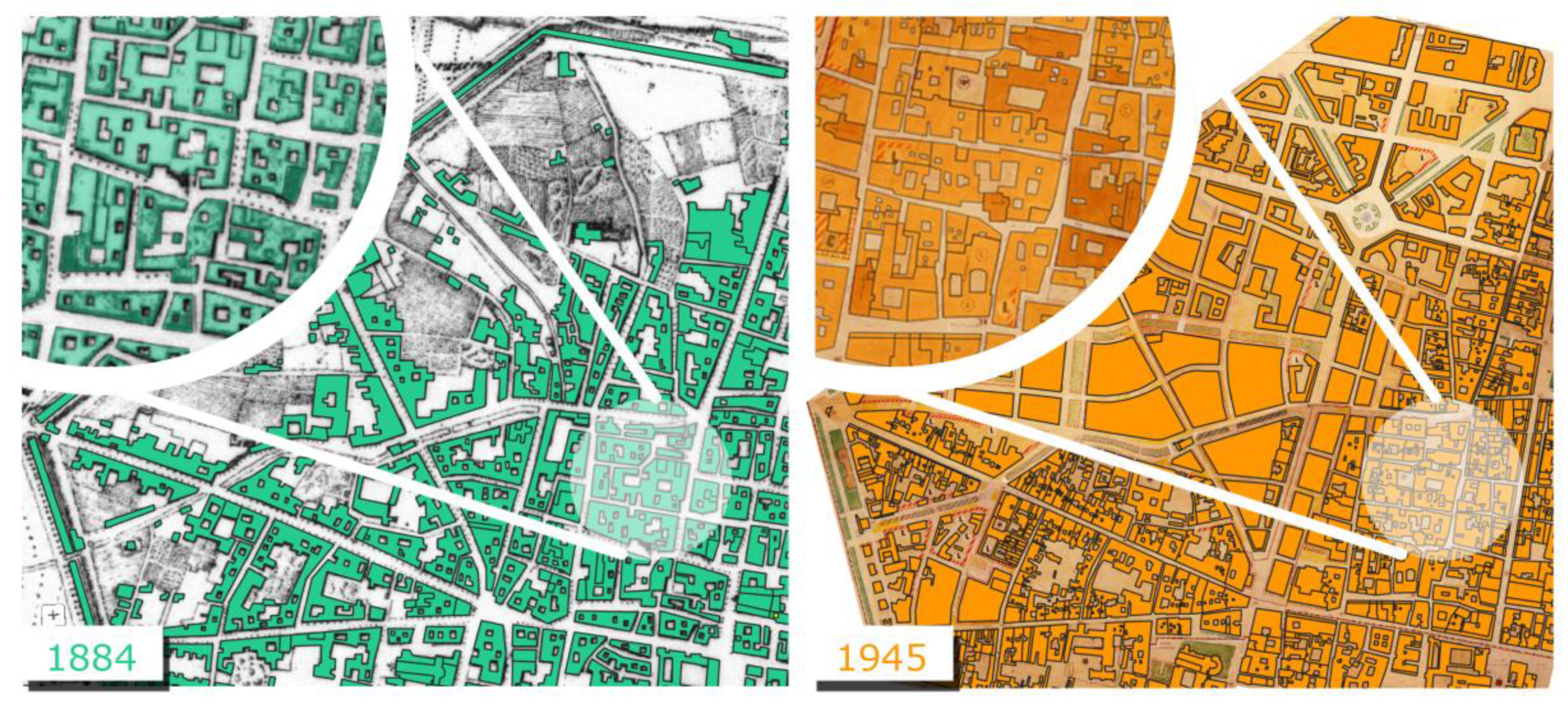
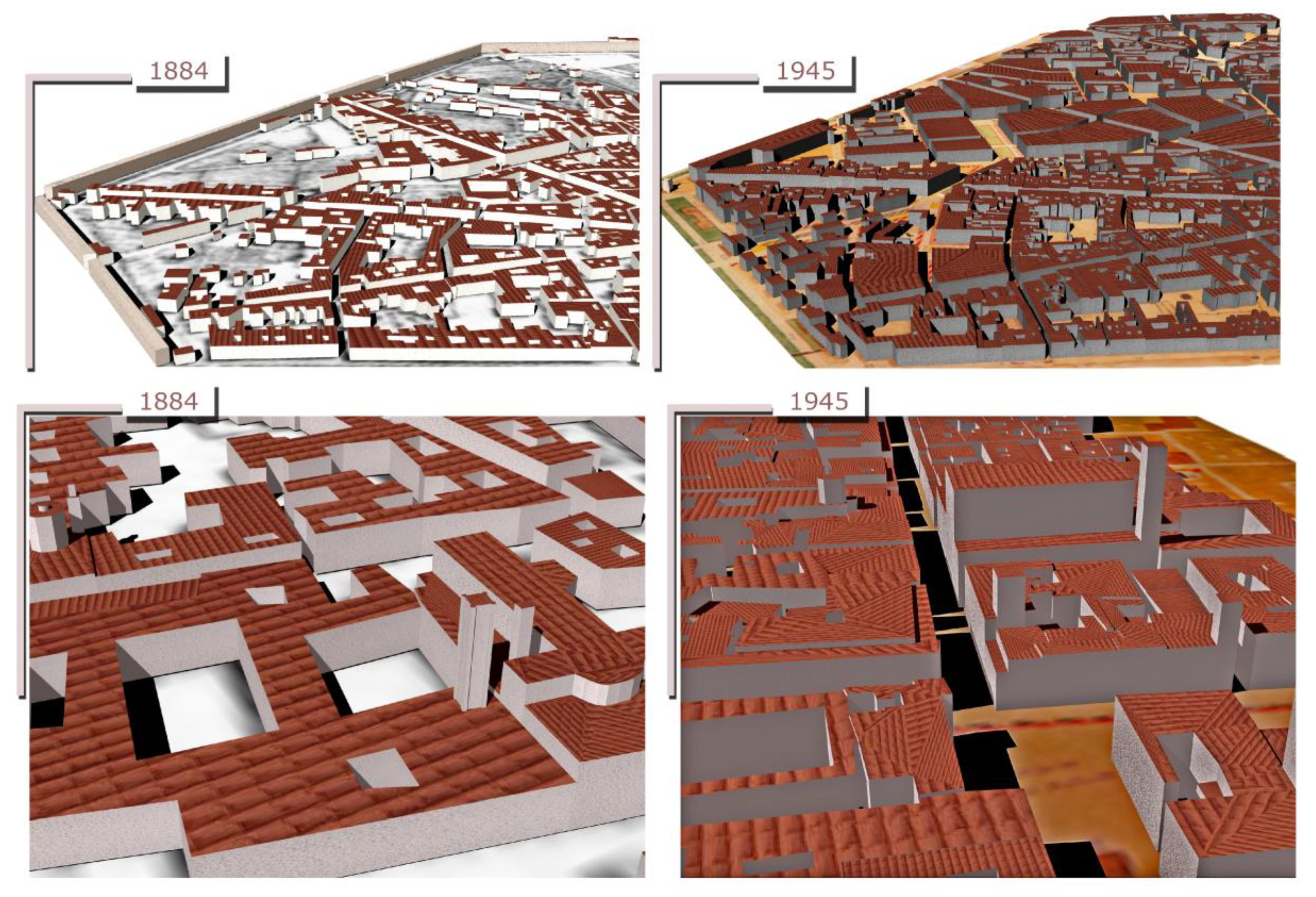
Applsci 11 01445 g002
Figure 3. The two digitised historical maps of Bologna (1884 and 1945).
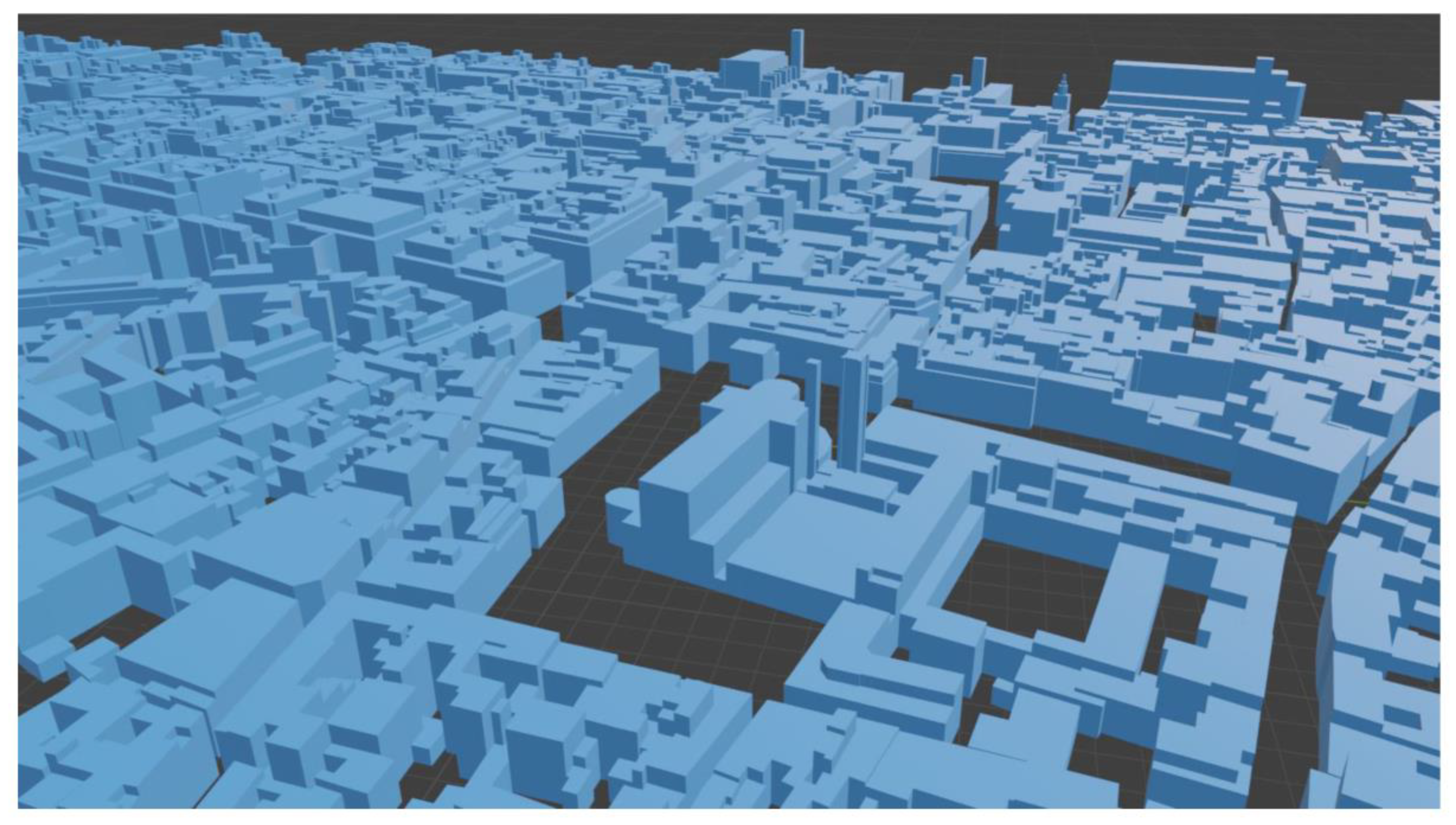
Applsci 11 01445 g003
Figure 4. A view of the LoD1 buildings in Bologna generated from the actual (2017) topographic data available as open data.
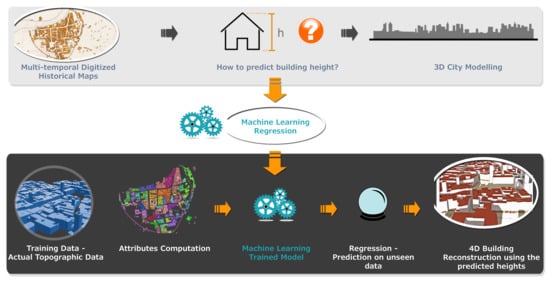
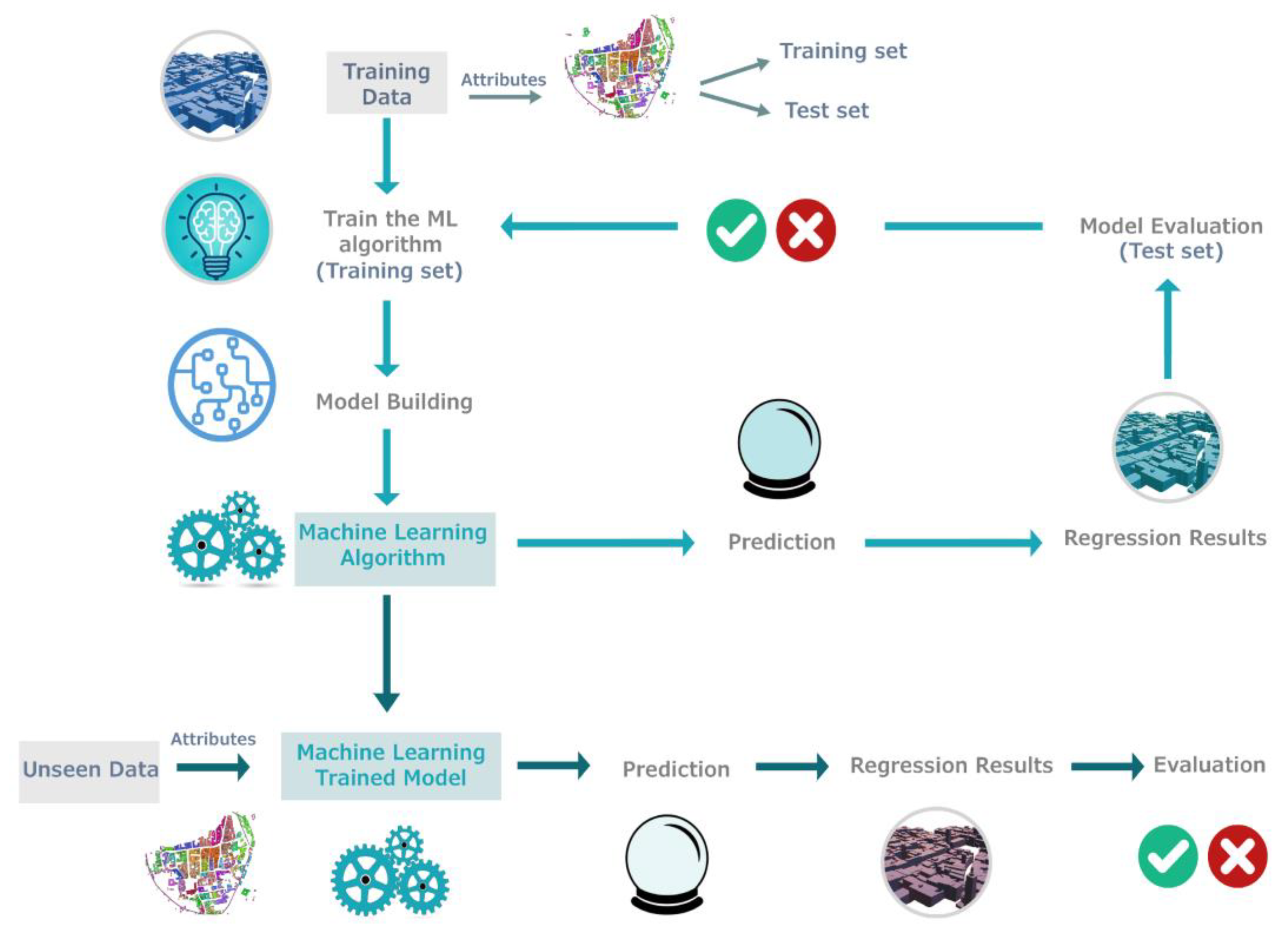
Applsci 11 01445 g004
Figure 5. The general workflow based on machine learning regression to learn building heights.
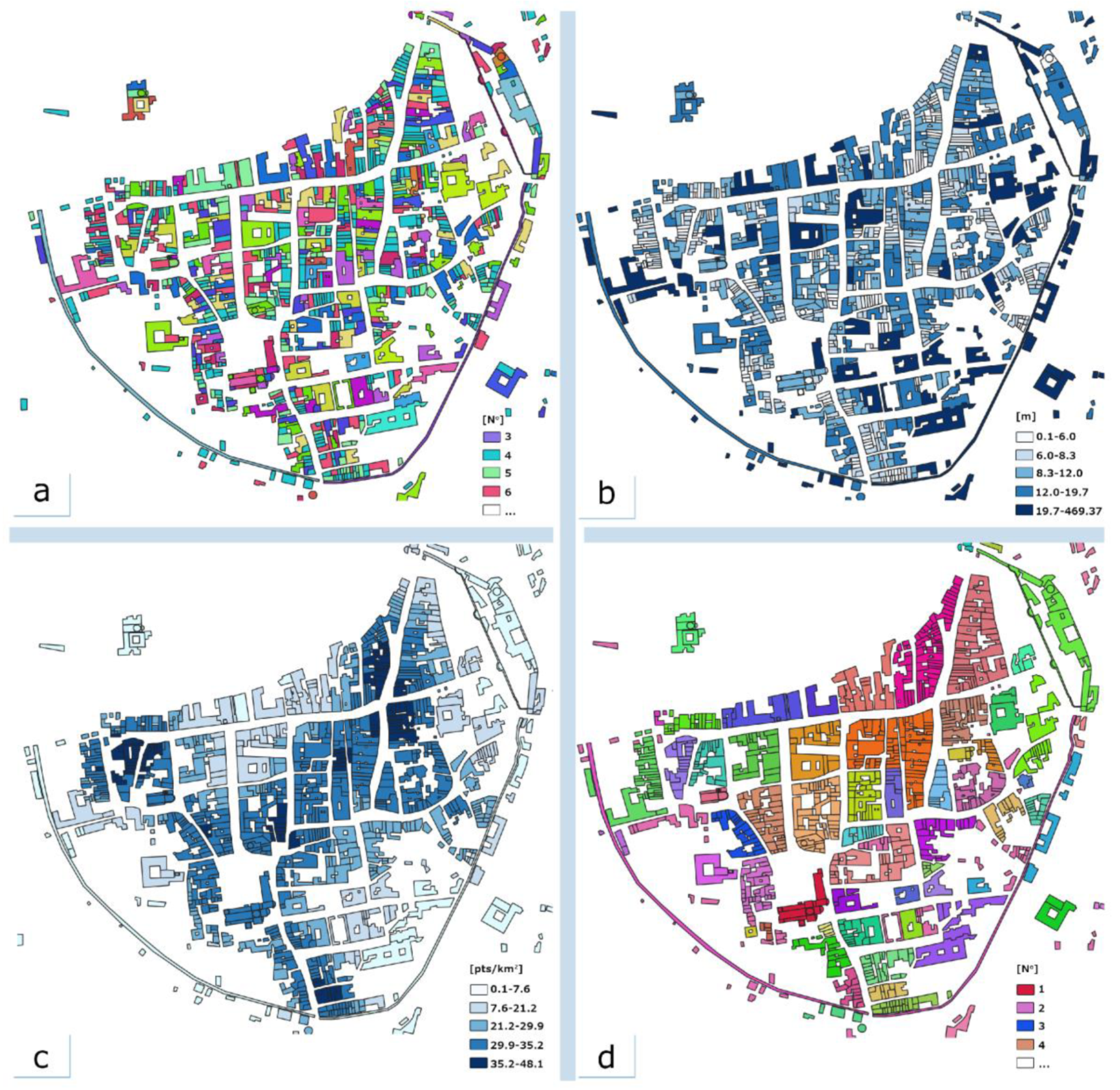
Applsci 11 01445 g005
Figure 6. Examples of attributes (predictors) computed for the Trento 1851 dataset: number of vertices (a); the distance of the polygon centroids from the nearest centroids (b); kernel density value—radius 100 m (c); groups (d). In (a) and (d) each colour corresponds to the computed (a) or assigned (d) numerical value. In (b) and (c), classes are colourised with a graduated scale.
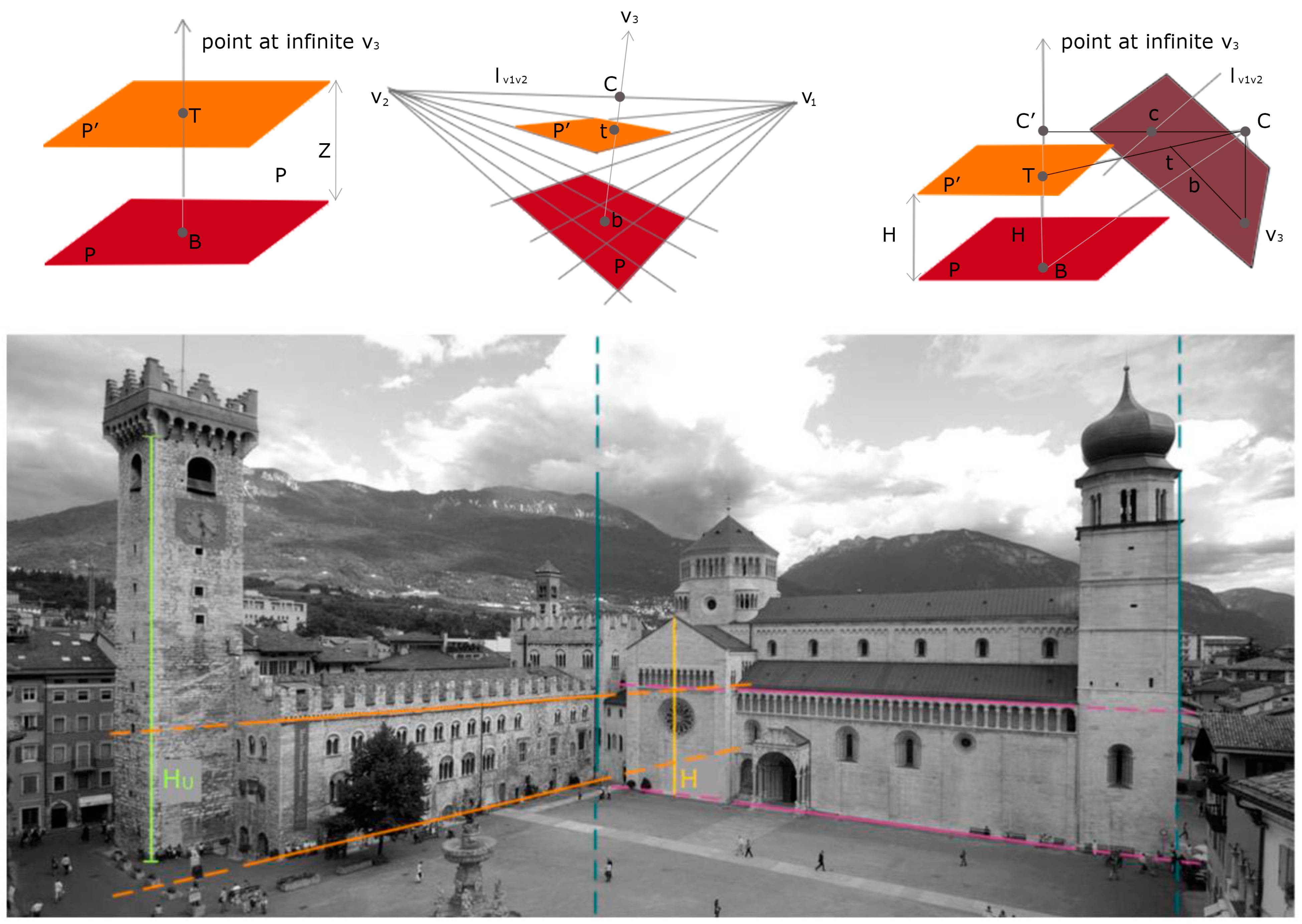
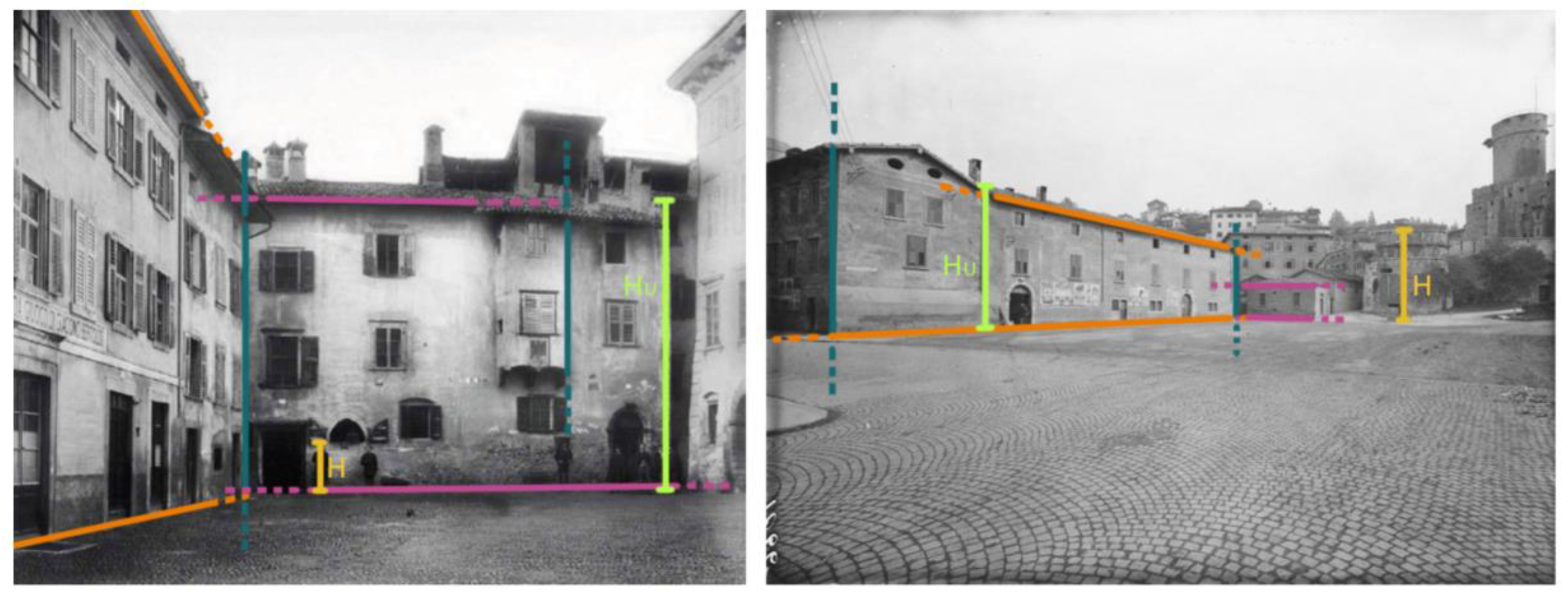
Applsci 11 01445 g006
Figure 7. Alignment of four points defining a cross-ratio invariant in image and object space (top). An example of height computation, deriving first the three vanishing points and then the unknown distance HU from the known H (bottom).
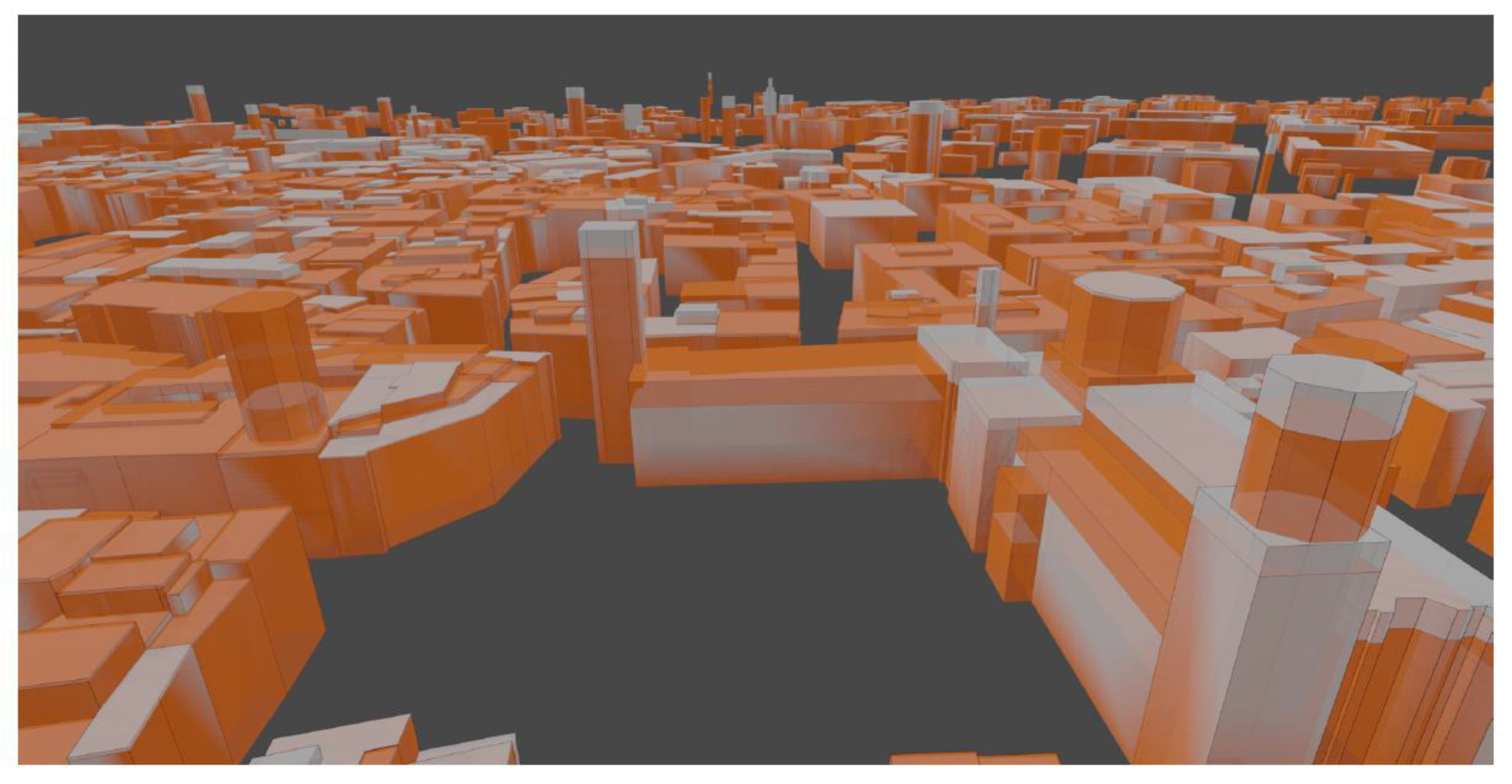
Applsci 11 01445 g007
Figure 8. 3D view of the inferred building heights (orange) with respect to the ground truth data (white) for Trento. Despite metrics indicating acceptable accuracy (Table 5), a visual check highlights gross errors mainly on towers.
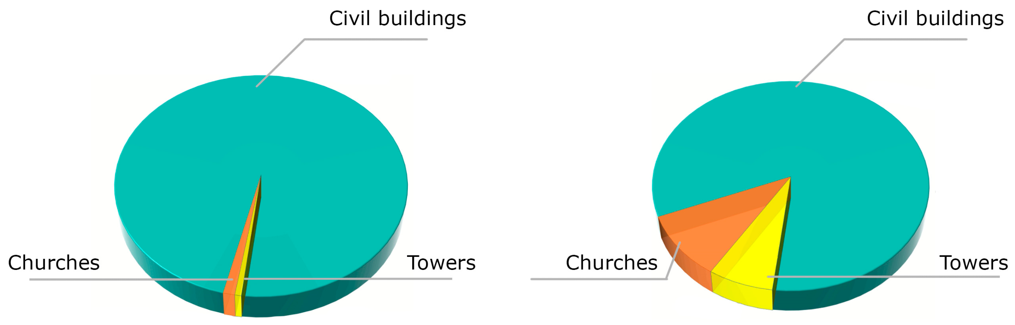
Applsci 11 01445 g008
Figure 9. Data distribution before (left) and after (right) adding synthetic data for the under-represented classes in the Trento dataset.
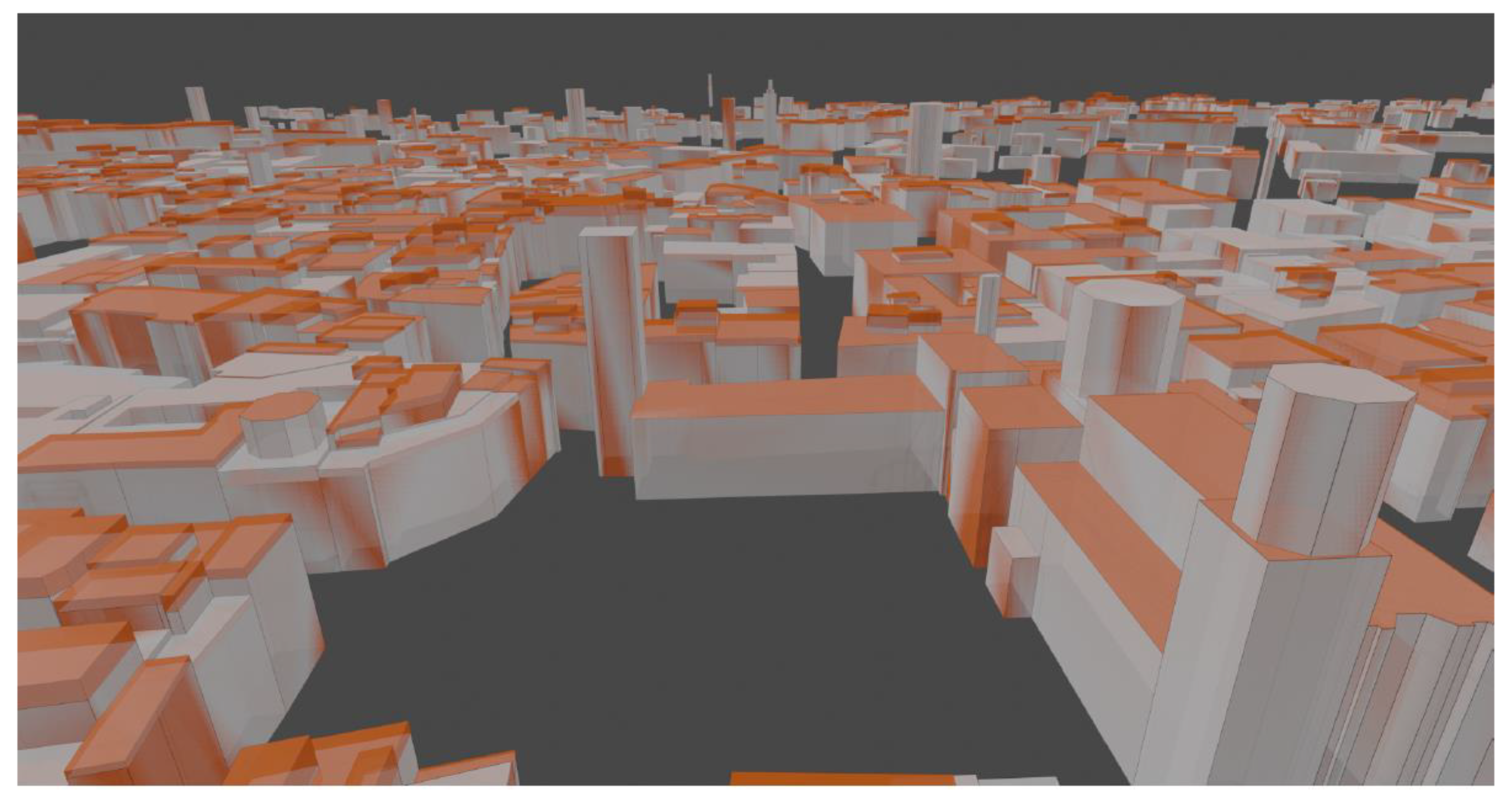
Applsci 11 01445 g009
Figure 10. 3D view of the inferred building heights (orange) in Trento with respect to the ground truth data (white) after data augmentation. The visual inspection shows a relevant reduction of the errors on towers and churches.
Applsci 11 01445 g010
Figure 11. Two examples of single-view-metrology applied to historical photos in Trento to determine heights of buildings not present anymore in the actual topographic database.
Applsci 11 01445 g011
Figure 12. Overviews of the generated multi-temporal 3D buildings (LoD1) using machine learning and historical maps for the Trento case study.
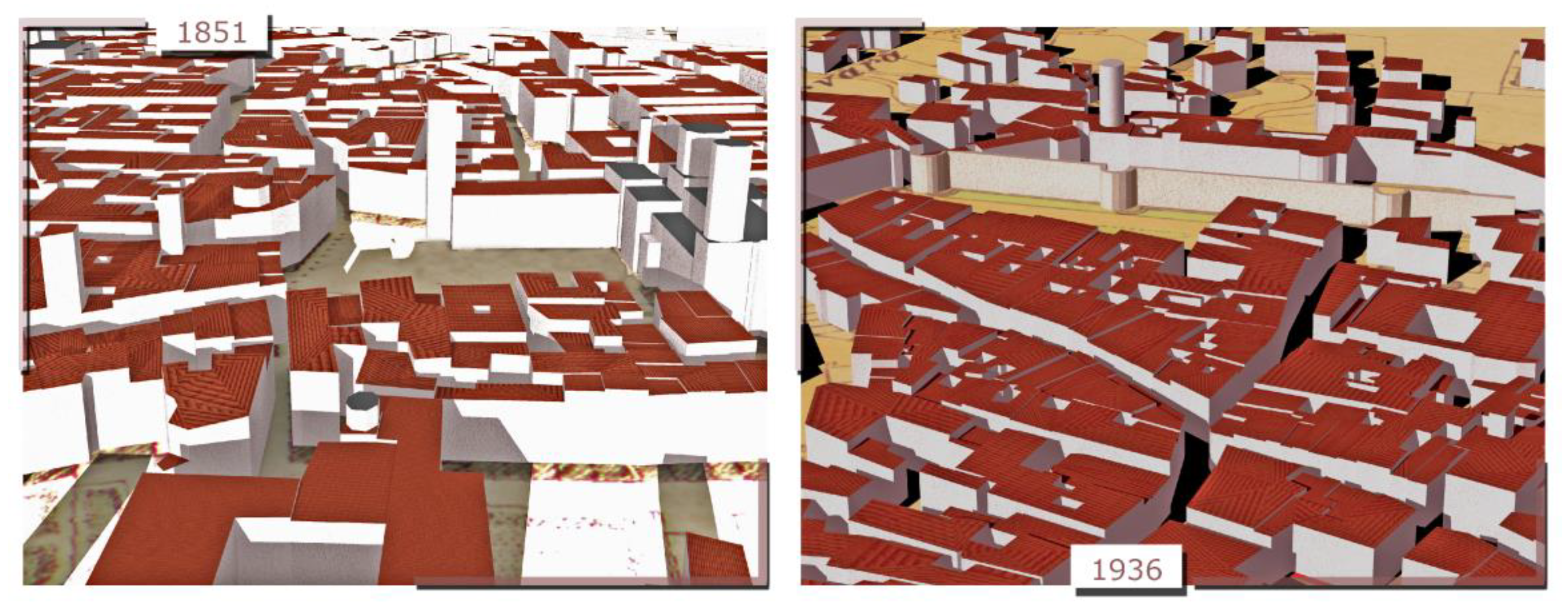
Applsci 11 01445 g012
Figure 13. Closer views of inferred 3D buildings in Trento in 1851 and 1936.
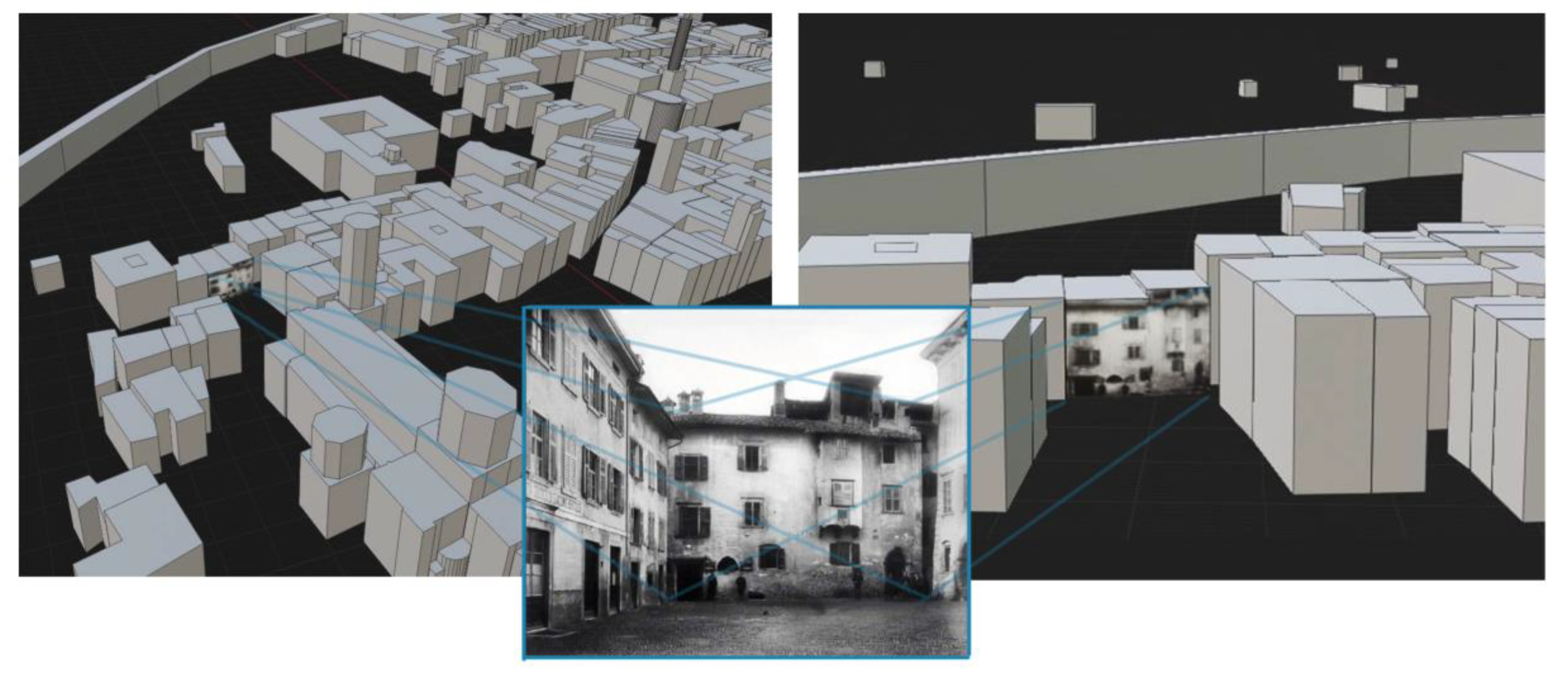
Applsci 11 01445 g013
Figure 14. An example of an historical photo used to texture a 3D building in Trento in 1887.
Applsci 11 01445 g014
Figure 15. Multi-temporal 3D reconstruction of Bologna with building heights inferred using machine learning and historical maps (1884 and 1945).
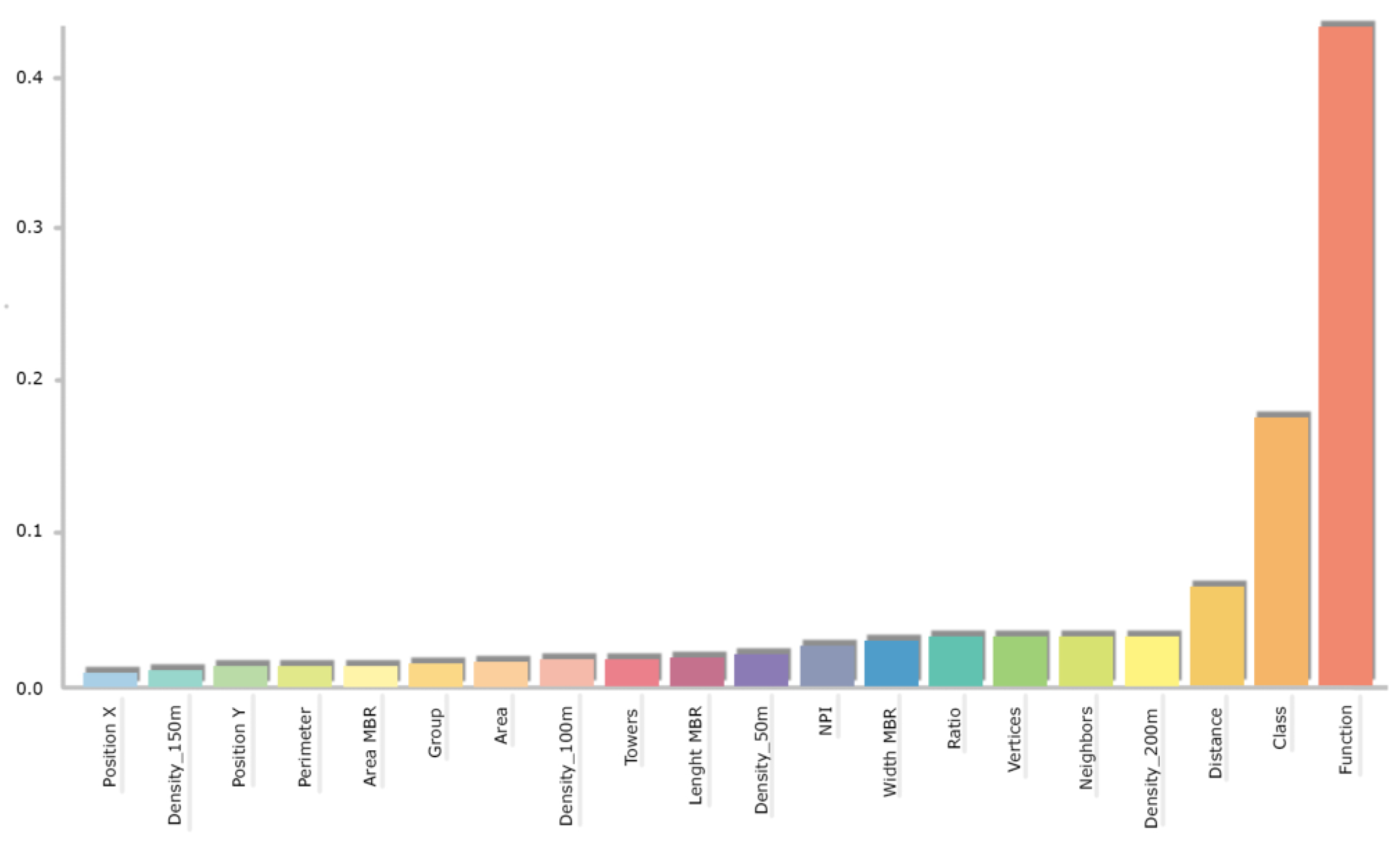
Applsci 11 01445 g015
Figure 16. Predictors importance of the Random Forest method in the Trento dataset. The most relevant are function (e.g., civil or religious), class (e.g., churches, palaces, castle), and distance (from a polygon’s centroid from the nearest centroid). On the y-axis, the features importance score is given, i.e., the normalised average scores indicating the weighted variance decrease in a decision tree.
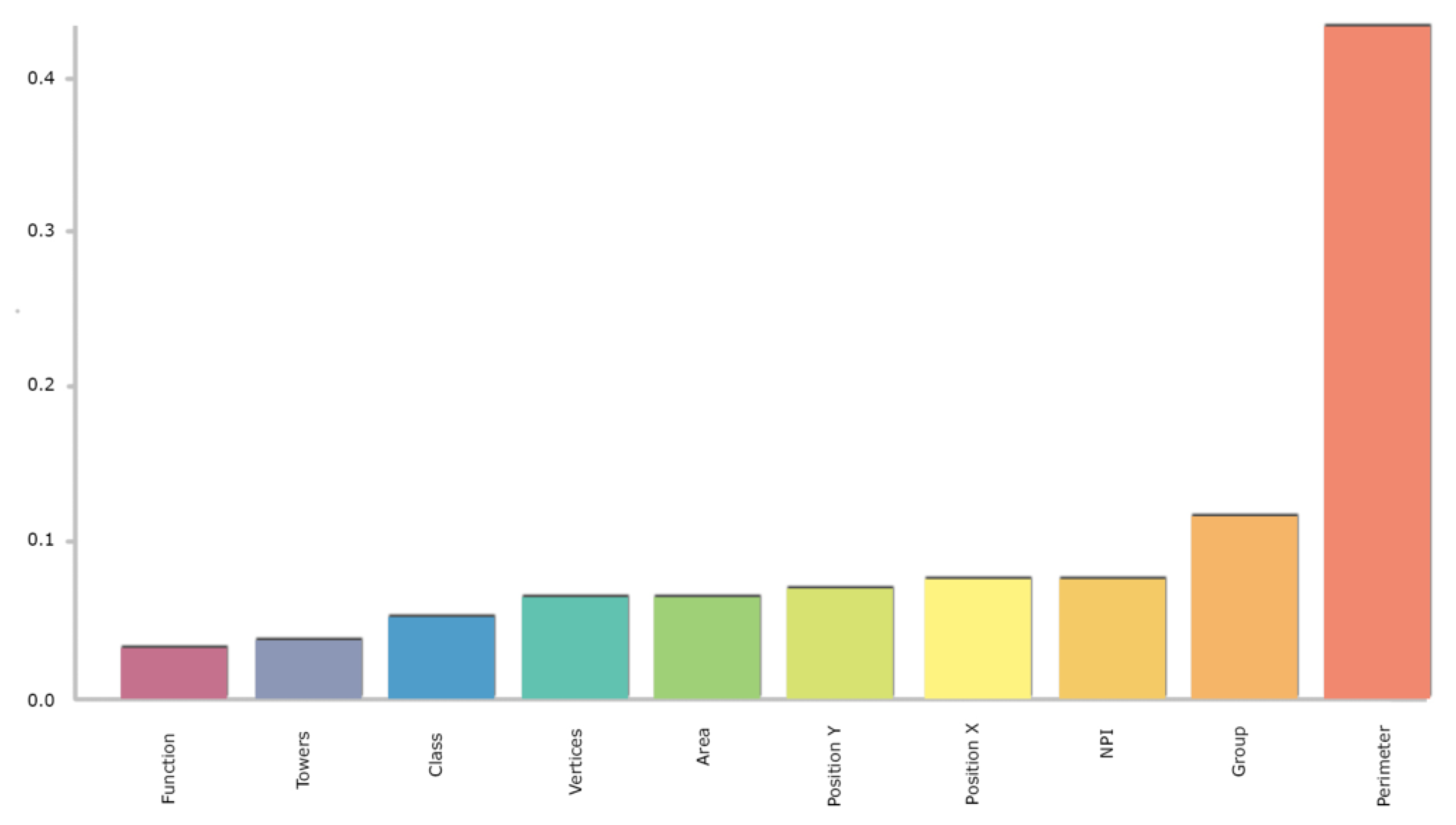
Applsci 11 01445 g016
Figure 17. Feature importance of the Random Forest method and RFE in the Trento dataset.
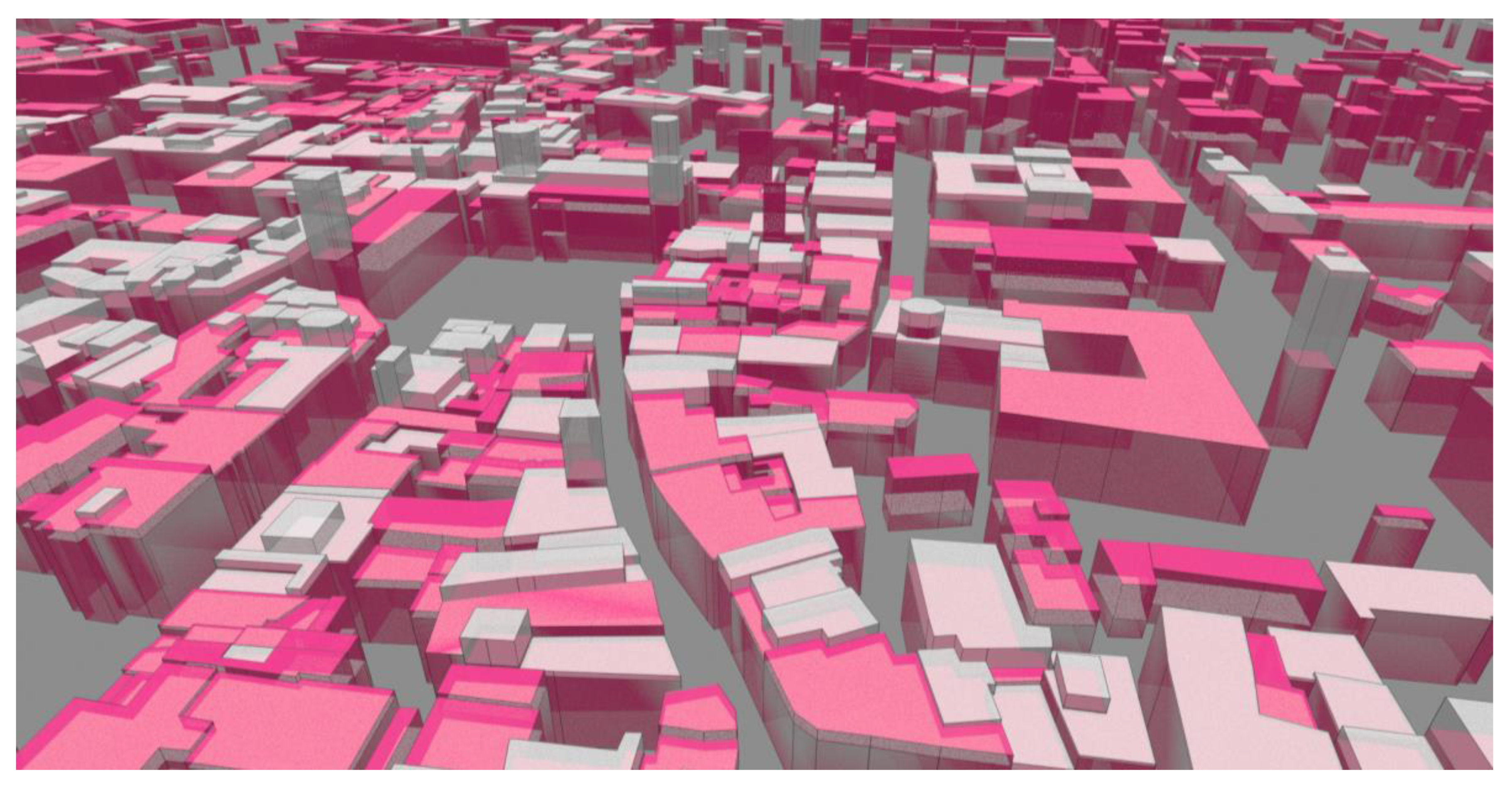
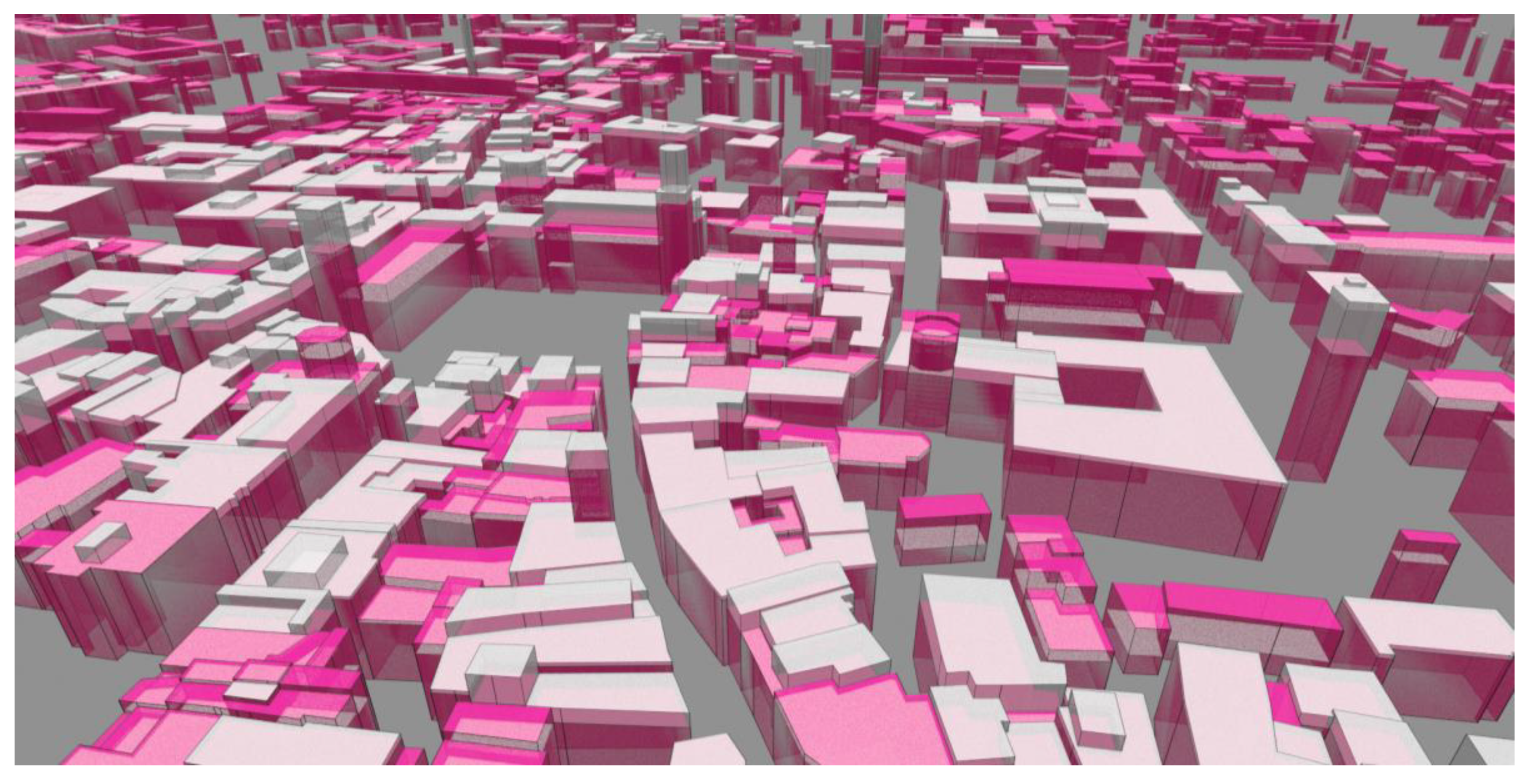
Applsci 11 01445 g017
Figure 18. 3D view of the inferred building heights (pink) in Trento with respect to the ground truth data (white), using the actual Bologna dataset as training. Training contains augmented data.
Applsci 11 01445 g018
Figure 19. 3D view of the inferred building heights (pink) in Trento with respect to the ground truth data (white), using the actual Bologna dataset as training. Data augmentation was removed from the training set.
Applsci 11 01445 g019
Table 1. The number of polygons and their average area in the four digitised historical maps and in the actual topographic data (2016).
DatasetTotal n. of Polygons Average Polygons Area (m2)
18511274197.18
1887632499.97
19081685238.24
19363112236.62
Actual4537 149.87
Table 2. The actual (2016) topographic data of man-made structures available for Trento.
DatasetTotal n. of PolygonsAverage Polygons Area (m2)Average Height (m)Median Height (m)St. Deviation (m)
Actual4537149.8712.2612.415.36
Table 3. The number of polygons and their average area in the two digitised maps and in the actual topographic data (2017).
DatasetTotal n. of Polygons Average Polygons Area (m2)
18844821750.35
19451174738.62
Actual3241215.04
Table 4. The actual topographic data (2017) for Bologna, used as training data and ground-truth.
DatasetTotal n. of PolygonsAverage Polygons Area (m2)Average Height (m)Median Height (m)St. Deviation (m)
Actual3241215.0414.7114.006.43
Table 5. Accuracy evaluation of the compared regressors for the Trento dataset.
RegressorRMSE TEST (m)MAE TEST (m)R2 TESTMedian (m)St. Dev. (m)
Linear5.564.38−0.080.686.13
Random Forest3.792.880.49−0.052.41
CatBoost4.033.050.43−0.023.05
Support Vector4.883.810.160.004.69
Multilayer Perceptron4.263.200.36−0.093.64
Table 6. Accuracy evaluation of the compared regressors for the Bologna dataset.
RegressorRMSE TEST (m)MAE TEST (m)R2 TESTMedian (m)St. Dev. (m)
Linear7.646.06−0.36−0.877.57
Random Forest4.673.640.49−0.062.95
CatBoost4.763.690.470.002.70
Support Vector4.884.100.330.055.03
Multilayer Perceptron4.943.180.430.074.31
Table 7. Data distribution for the Trento and Bologna dataset.
DatasetTotal n. of Polygons TowersChurchesCivil Buildings
Trento4537 30 (~1%)53 (~1%)4454 (~98%)
Bologna324130 (~1%)21 (~1%)3190 (~98%)
Table 8. Data distribution after the inclusion of synthetic data for the under-represented classes.
Dataset
Data Augmentation
Total n. of PolygonsTowersChurchesCivil Buildings
Trento5369379 (~7%)531 (~10%)4454 (~83%)
Bologna3553176 (~5%)136 (~4%)3241 (~91%)
Table 9. Accuracy evaluation of the regressor methods on the Trento dataset after data augmentation.
RegressorRMSE TEST (m)MAE TEST (m)R2 TESTMedian (m)St. Dev. (m)
Linear 5.904.69−0.151.156.66
Random Forest 3.592.830.570.002.07
CatBoost3.762.950.530.002.61
Support Vector5.304.240.07−0.065.44
Multilayer Perceptron4.173.200.43−0.053.57
Table 10. Accuracy evaluation of the regressor methods on the Bologna dataset after data augmentation.
RegressorRMSE TEST (m)MAE TEST (m)R2 TESTMedian (m)St. Dev. (m)
Linear 8.526.810.04−0.758.51
Random Forest 4.523.540.490.002.72
CatBoost4.643.660.520.002.49
Support Vector5.153.490.410.004.78
Multilayer Perceptron4.833.790.48−0.023.91
Table 11. Metrics evaluation of the Random Forest performance on the four historical datasets of Trento, considering twenty unaltered buildings digitised in all the maps as the test set.
Historical Map-YearRMSE (m)MAE (m)R2Min Error (m)Max Error (m)Median (m)St. Dev. (m)
18510.961.130.972.951.751.090.74
18872.862.250.920.076.351.521.77
19081.801.500.96−2.783.911.180.99
19361.671.400.97−2.623.201.140.90
Table 12. Metrics evaluation of the Catboost performance on the four historical datasets of Trento, considering twenty unaltered buildings as the test set.
Historical Map-YearRMSE (m)MAE (m)R2Min Error (m)Max Error (m)Median (m)St. Dev. (m)
18514.913.220.83−2.9313.872.023.71
18876.093.930.670.2417.152.314.65
19084.663.080.81−3.1214.382.113.49
19365.803.310.70−2.7219.021.384.76
Table 13. Evaluation on eight disappeared buildings visible in historical photos: heights predicted with Random Forest were compared with single-view-metrology heights and metrics derived.
DatasetRMSE (m)MAE (m)Median (m)St. Dev. (m)
Trento1.411.28−0.831.29
Table 14. Metric evaluation of the Random Forest prediction on the two historical datasets of Bologna, considering as a test set ten unaltered buildings digitised in both maps.
Historical Map-YearRMSE (m)MAE (m)R2Min Error (m)Max Error (m)Median (m)St. Dev. (m)
18842.672.350.972.101.090.730.54
19451.711.630.99−1.666.351.521.89
Table 15. Metric evaluation of the Catboost prediction on the two historical datasets and ten unaltered buildings as the test set.
Historical Map-YearRMSE (m)MAE (m)R2Min Error (m)Max Error (m)Median (m)St. Dev. (m)
18847.566.810.88−2.3010.928.393.28
19457.987.050.83−1.9812.387.763.70
Table 16. Evaluation metrics for the Trento dataset with and without a recursive feature elimination (RFE) approach.
RegressorN. of FeaturesRMSE TEST (m)MAE TEST (m)R2 TESTSt. Dev. (m)
Random Forest—without RFE203.592.830.572.07
Random Forest—with RFE103.832.990.512.18
Table 17. Evaluation metrics for the Bologna dataset with and without an RFE approach.
RegressorN. of FeaturesRMSE TEST (m)MAE TEST (m)R2 TESTSt. Dev. (m)
Random Forest—without RFE204.523.540.492.72
Random Forest—with RFE104.593.540.532.76
Table 18. Accuracy evaluation with the Random Forest regressor, training on Bologna data, and predicting on Trento dataset, and vice-versa. In this test, positional attributes were removed, and augmented data were employed for both cases.
Dataset PredictionDataset TrainingRMSE TEST (m)MAE TEST (m)R2 TESTMedian (m)St. Dev. (m)
Trento Bologna4.603.570.530.002.77
BolognaTrento3.732.950.540.002.15
Table 19. Accuracy evaluation with the Random Forest regressor and inverted training data. In this case, augmented data were removed from the training.
Dataset PredictionDataset TrainingRMSE TEST (m)MAE TEST (m)R2 TESTMedian (m)St. Dev. (m)
Trento Bologna3.902.980.47−0.032.49
BolognaTrento4.753.700.47−0.092.99
Publisher’s Note: MDPI stays neutral with regard to jurisdictional claims in published maps and institutional affiliations.

