Article

Statistical Uncertainty of DNS in Geometries without Homogeneous Directions

1
Reactor Engineering Division, Jožef Stefan Institute, Jamova Cesta 39, SI-1000 Ljubljana, Slovenia
2
Curiosity Group, Pprime Institute, Université de Poitiers, CNRS, ISAE-ENSMA-Téléport 2-Bd. Marie and Pierre Curie B.P. 30179, 86962 Futuroscope Chasseneuil CEDEX, France
*
Authors to whom correspondence should be addressed.
Appl. Sci. 2021, 11(4), 1399; https://doi.org/10.3390/app11041399
Submission received: 30 December 2020 / Revised: 28 January 2021 / Accepted: 29 January 2021 / Published: 4 February 2021
(This article belongs to the Special Issue Applications of Liquid Metals II)

Abstract

:
In this paper, we present uncertainties of statistical quantities of direct numerical simulations (DNS) with small numerical errors. The uncertainties are analysed for channel flow and a flow separation case in a confined backward facing step (BFS) geometry. The infinite channel flow case has two homogeneous directions and this is usually exploited to speed-up the convergence of the results. As we show, such a procedure reduces statistical uncertainties of the results by up to an order of magnitude. This effect is strongest in the near wall regions. In the case of flow over a confined BFS, there are no such directions and thus very long integration times are required. The individual statistical quantities converge with the square root of time integration so, in order to improve the uncertainty by a factor of two, the simulation has to be prolonged by a factor of four. We provide an estimator that can be used to evaluate a priori the DNS relative statistical uncertainties from results obtained with a Reynolds Averaged Navier Stokes simulation. In the DNS, the estimator can be used to predict the averaging time and with it the simulation time required to achieve a certain relative statistical uncertainty of results. For accurate evaluation of averages and their uncertainties, it is not required to use every time step of the DNS. We observe that statistical uncertainty of the results is uninfluenced by reducing the number of samples to the point where the period between two consecutive samples measured in Courant–Friedrichss–Levy (CFL) condition units is below one. Nevertheless, crossing this limit, the estimates of uncertainties start to exhibit significant growth.

1. Introduction

The present work represents a synthesis on the statistical uncertainties of the results obtained in a direct numerical simulation (DNS) of flow in a channel and a flow over a confined backward-facing step (BFS). Some of the results of the DNS in BFS were already presented by Oder et al. [1]. To be able to compare results of DNS to experiments and other simulations, the results are presented in a form of averages. As is well known [2], there are two errors attributed to data obtained in a DNS. The more widely known are the errors connected to spatial and temporal resolution. The scale of these errors is usually shown with results obtained with different spatial (temporal) resolutions or with comparisons of smallest turbulent scales to the spatial resolution.
The second error is accumulated due to finite interval when performing time integration for statistically steady flows. This error drops as a square root of integration time ( T 1 / 2 ) and in most simulations, defines the duration of DNS, as well as the computational cost of the DNS. To amend the high computational costs, in simulations with homogeneous directions, these can be utilised to speed-up the reduction of statistical uncertainty by, in addition to temporal integration also performing spatial integration over the homogeneous directions. With such method, the simulation can be one or even two orders of magnitude less demanding. To clarify, according to Pope [3], homogeneous directions are directions in which statistical quantities do not vary with translation. Similarly, a statistical steady state of a turbulent flow is a state where statistical quantities do not vary with translation of time averaging interval.
Vreman and Kuerten [4] performed a detailed study of accuracies of different DNS databases of channel flow. The analysis was focused on spatial resolutions, as well as different algorithms. The study showed that higher statistical moments require better spatial resolutions to achieve the same level of accuracy as the first moments of statistics. More recently, Vinuesa et al. [5] performed an analysis of how starting time of averaging and the averaging time affects the convergence of statistical quantities in a DNS. They also explored the effects of different sampling rates. Ries et al. [6] in a recent Large Eddy Simulation (LES) study found that due to large integral time scales, longer averaging times are needed in regions near the walls. As noted by Andrade et al. [7], it would be of interest to the turbulent community if more attention would be dedicated to the uncertainties and convergence criteria.
The DNS results exposed here were presented in the papers [1,8]; the details of the numerical setups can be found there. Only a short description will be given here. A more thorough presentation of all the parameters of the BFS DNS can also be found in [9]. Therefore, we also compared the accuracy of the Nek5000 solver in the channel upstream of the step with the same distribution of elements to the results obtained with a conservative pseudospectral method that was used in the channel simulation. If the reader is interested in a comparison of Reynolds Averaged Navier Stokes (RANS) simulation and LES results, they can be found in [10]. In the present paper, we rather focus on the statistical uncertainties found in the channel flow with two homogeneous directions, and on the BFS flow with no homogeneous directions. In Section 2 we present the numerical setups of channel flow DNS and BFS DNS. In Section 3 we present the results, first for the channel flow and then for the flow over the BFS. The results for the BFS are first presented as profiles with added error bars and later we present results in 49 monitor points. The concluding remarks are in Section 4.

2. Numerical Model

A standard incompressible Navier–Stokes system of equations, without gravity, was used in both cases:
u = 0 ,
u t + ( u ) u = p + 1 R e 2 u ,
where u is the velocity vector field, p is the pressure and R e is the appropriate Reynolds number.

2.1. Channel Flow

The details of numerical set-up for a channel flow are described by Tiselj et al. [8]. The infinite channel corresponds to the flow between two infinite parallel walls; it allows for implementation of periodic boundary conditions in x and z directions only: in the y direction the domain is limited by walls. The time and space averaged results are thus one-dimensional. The domain in the particular case considered in the present paper is 4 π units long, 2 units tall and 4 π / 3 units wide
The above Navier–Stokes system of equations was transformed into a conservative form that can be used with periodic boundary conditions, by adding an artificial force term in the momentum equation, which drives the flow through the channel. The procedure can be found in various sources, however, we suggest the one by Kawamura et al. [11]. The friction Reynolds number Re τ in the simulation was set to 180. The equations are solved with a pseudo-spectral scheme. Fourier series are used in x and z directions, while Chebyshev polynomials are used in the y direction. 128 modes were used in x and z directions each, while 129 modes were used in the y direction.
Second-order accurate time differencing (Crank–Nicolson scheme for diffusive terms and Adams–Bashforth scheme for other terms) is used with maximum Courant number kept at approximately 0.1. The aliasing error is removed with computation of the nonlinear terms on a grid 1.5 times finer in all directions. The computer code is based on the code developed by [12], which was later modified by [13]. The code was used and verified in simulations of [14,15,16].
In the channel, results are presented with two types of averaging:
  • “standard” averaging used in channel flow DNS studies, where time averaging is supported with spatial averaging in two homogeneous directions. At each time step, the spatially averaged values are stored for uncertainty analyses.
  • time averaging only in a selected line, perpendicular to the channel walls. In monitor points on this line, the whole history of velocity and pressure is saved from which the averages and uncertainties of these averages can be estimated.
The uncertainty is calculated with the help of ar program from arsel library [2]. In a similar way to the channel case, the monitor point data is saved at each time step. In the post-processing phase, the ar program is used to estimate the decorrelation time T 0 or associated number of time steps N 0 , which is the time or number of time steps, respectively, when the variable samples become independent. More rigorously, T 0 is the time when the estimated autocorrelation function becomes insignificant. This technique is explained by Oliver et al. [2]. The sampling error or the estimate of uncertainty σ of a variable x is:
σ 2 = N 0 N ( N N 0 ) i = 1 N ( x i x ) 2 ,
where x is the estimation of the average, derived from the N samples. In the present study, the samples are equidistant in time. The uncertainty still has the dependency 1 / N at values for N N 0 .

2.2. Backward Facing Step Flow

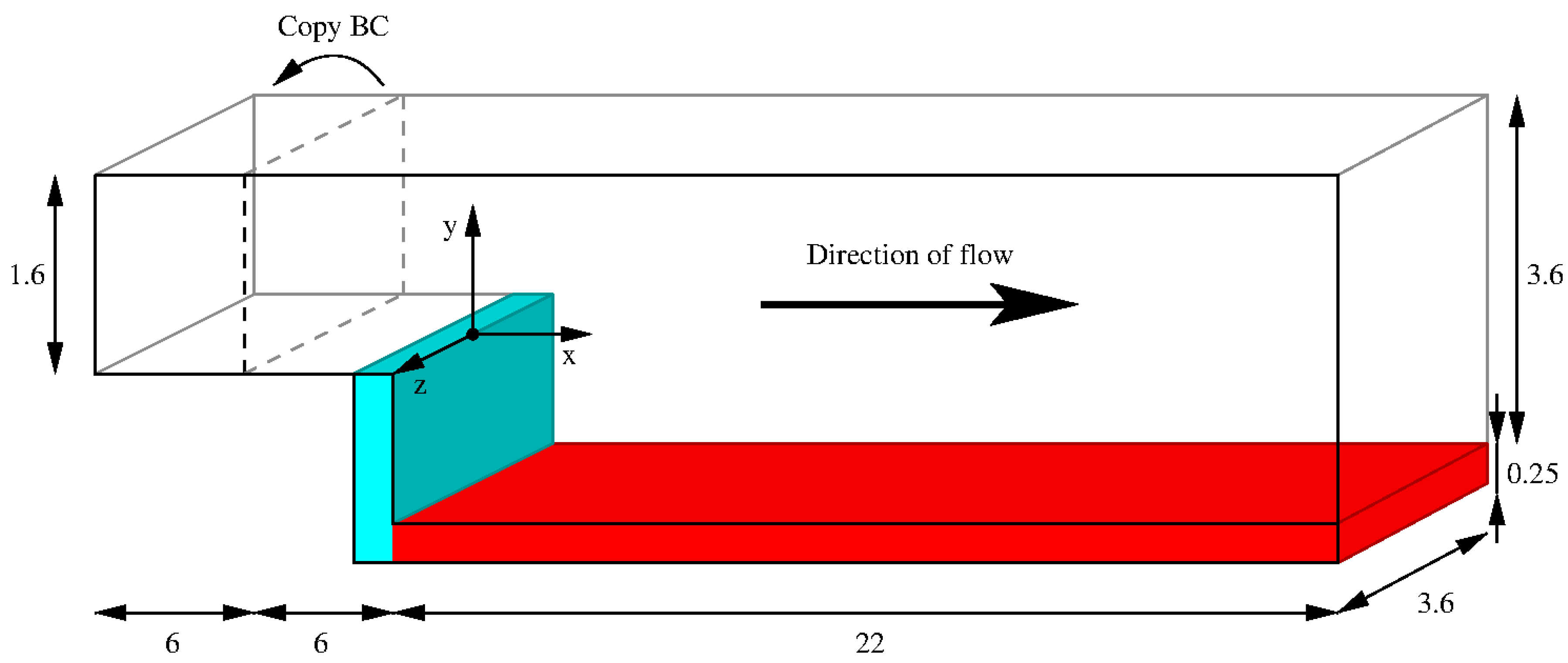
The details of the numerical set-up of the BFS case are described by Oder et al. [1]. A sketch of the domain is shown in Figure 1. The flow enters at left into the narrow duct. Twelve dimensionless units downstream of the inflow, the duct expands into a wider rectangular duct. The outflow is located 22 dimensionless units downstream of the step. All the boundaries of the domain, except for the inflow and outflow, are no-slip velocity boundary conditions. The no-slip velocity boundary condition is also applied at the lateral sides. The thermal domain is a bit larger since it includes two solid walls: the step wall (cyan) and the heater (red). The thickness of the walls is 0.25 dimensionless units. The heater contains an internal volumetric heat source. The outer parts of the domain are thermally insulated, while at the intersection of fluid and solid domain a conjugate heat transfer boundary condition is used.
The standard incompressible Navier–Stokes system of equations, without gravity effects, is solved, however, here a constant mass influx was used as a boundary condition. The appropriate Reynolds number based on bulk velocity at the inflow and hydraulic diameter at the inflow was set to 7089. The calculated average friction Reynolds number in the channel upstream was around 207. In addition to the Navier–Stokes system of equations, the energy equations for two passive scalars with Prandtl numbers of 0.005 and 0.1 are also solved for. Buoyancy is neglected, as are thermally dependant material properties of fluid and walls.
The equations are solved using the spectral element method implemented in the open source code nek5000, which is developed at the Argonne National Laboratory. The elements are smaller at the walls and larger in the middle of the channels. In the x direction the elements are of constant 0.25 length units. In the y direction the element sizes are varying from 0.044 to 0.115, while in the z direction the sizes vary from 0.047 to 0.210. Within each element there are seven collocation points in each direction. The calculations are performed with dealiasing with 11 collocation points in each direction. The PN/PN formulation is used, that is, the mesh for pressure variable is the same as the mesh for velocity. Second order time marching scheme (EXT2) is used, however, the time step is chosen so that the CFL number is oscillating around 0.1.
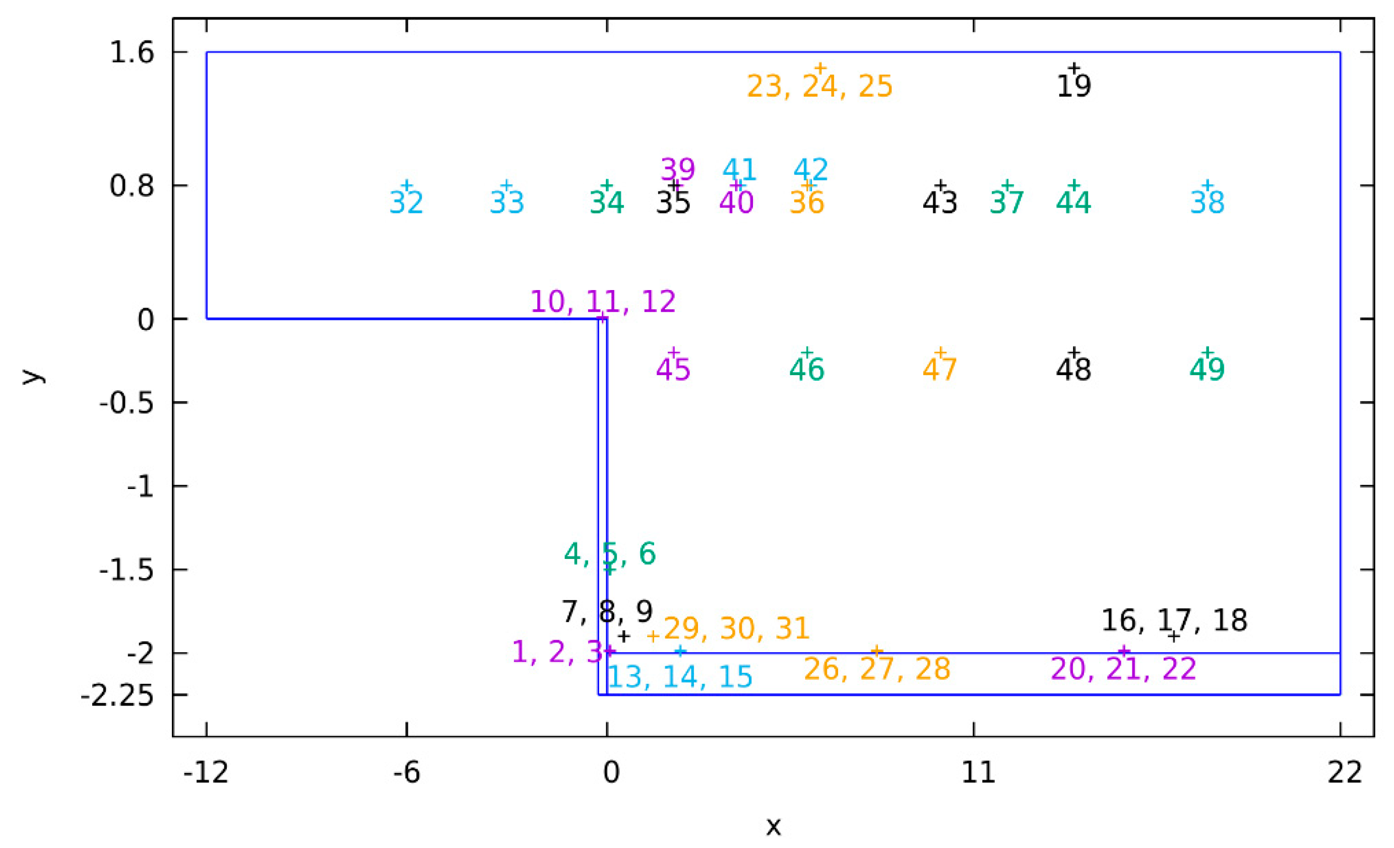
Since there are no homogeneous directions in the step geometry, the results are presented in a different manner. 49 positions were selected in which the values of velocity, pressure and the two passive scalars were exported at each time step. These 49 points are not computational points but, rather, the values there are obtained through spectral interpolation.
Figure 2 shows the distribution of monitor points in which we can calculate the statistical uncertainty associated with time averaging of DNS results. Their precise position is given in the Table A1 in the Appendix A. The position of each monitor point was chosen during the set-up of the DNS and during the initial runs. The positions were selected where during these preliminary runs, interesting features of the flow or temperature fields, such as maxima of components of turbulence fluctuations, averages, etc., were observed. Some points were also chosen as a means to determine the quality of the DNS.

3. Results

3.1. Uncertainties in Channel Flow

Once the statistical steady state is recognized, the temporal and spatial averaging of the results was performed. A rather generally accepted rule of thumb says that the uncertainty of the basic statistical profiles in DNS should be less than ~1%. However, a detailed study of Vreman [4] shows that it takes several hundred thousand time steps to achieve that target even in channel flow, where the statistical uncertainty is reduced also with the spatial averaging in two homogeneous directions. The corresponding number of time steps for the flows with a single homogeneous direction [17] is larger, and must be even larger in the geometries without homogeneous directions, where the only available type of averaging is averaging in time or ensemble averaging with several independent DNS runs performed in the same geometry.
Profiles of the key turbulent statistics with quantified statistical uncertainty shown in Figure 3 compare two types of averaging: much lower uncertainty is achieved when temporal averaging is combined with the spatial averaging in two homogeneous directions (in addition, the symmetry of the channel in the y direction was also utilised with spatial averaging). However, as can be clearly observed, the reduction of statistical uncertainty with spatial averaging is not universal across the domain. As can be observed for the mean stream wise velocity component the benefit of spatial averaging is insignificant in the middle of the channel, while it reduces the uncertainty almost by an order of magnitude at around y + ~ 10 . This could mean that our domain is not large enough. The effects of uneven reduction of statistical uncertainties across the domain are observed in all variables. The averaging time t+ was 54,000, and the time step was ∆t+ = 0.027. This is about 2 million time steps; however, only every tenth time step was used for averaging.
If the results shown in Figure 3 are applicable to an arbitrary turbulent flow without homogeneous directions, then reduction of statistical uncertainty requires typically millions of time steps and consequently large computational resources.
For some variables, for example Root-Mean-Square (RMS) of the streamwise velocity component, the peaks of mean values correspond with peaks of statistical uncertainty. This results in constant relative statistical uncertainties. For mean streamwise velocity component, this percentage changes through the domain, but is around few tenths of percent. However, in the case of Reynolds stress u v , which is expected to be zero in the middle of the channel, the statistical uncertainty has a finite non-zero value, which causes the relative statistical uncertainty to diverge. If we discard such cases, we can claim that with temporal averaging only, the relative statistical uncertainties are also an order of magnitude higher. If we only observe the peaks of statistical uncertainties, however, the statistical uncertainty of shown results is around few percent without spatial averaging and around few tenths of percent with spatial averaging.
The convergence rate of statistical uncertainties in channel flow DNS was explored by Andrade et al. [7] and more recently by Flageul and Tiselj [18]. Additionally, Flageul and Tiselj explained why statistical uncertainties of some global parameters converge with the rate, which is inversely proportional with averaging time.

3.2. Uncertainties in Flow over Backward-Facing Step (BFS)

Here we present the results in all the 49 monitor points that were used during the DNS of BFS. The data from the first 31 monitor points were averaged over 12 million time steps for the velocity, pressure and the passive scalar with Pr = 0.005 . Samples from monitor points 32 to 49 were averaged only over about 10 million time steps. The data for the second passive scalar, with Pr = 0.1 were averaged over 7 million time steps. These discrepancies are because of late addition of monitor points 32 to 49 to the simulation, and late addition of the second passive scalar, which also had to reach a statistical steady state. Note that the averaging intervals differ in beginning only, but have identical end of time integration. The detailed integration span for uncertainty estimation is given in Table 1.
Nevertheless, the profile data were obtained by integrating for the whole duration of 12 million time steps for velocity, pressure and passive scalar with Pr = 0.005 . Therefore the uncertainty estimation for monitor points 32–49 is a conservative estimate for uncertainties of the profiles. The profiles involving passive scalar with Pr = 0.1 were obtained from the same time span as uncertainty data.
The flow through time in the BFS case was approximately 60 dimensionless time units. With a time step of 4 × 10 4 dimensionless time units, this is equal to approximately 150 thousand time steps. Thus, our simulation spanned more than about 80 flow-through times.
The statistical steady state for the flow field and the passive scalar with Pr = 0.005 was determined with the help of volumetric averaging in the area downstream the step. No particular tools were used to determine this. Since the second scalar with Pr = 0.1 was added later in the simulation, the statistical steady state was determined separately. For the determination of the turbulent heat flux, the average velocity is needed. The shortened time integration interval was used to determine the average velocity that is used in the calculation of the turbulent heat flux for the passive scalar with Pr = 0.1 .
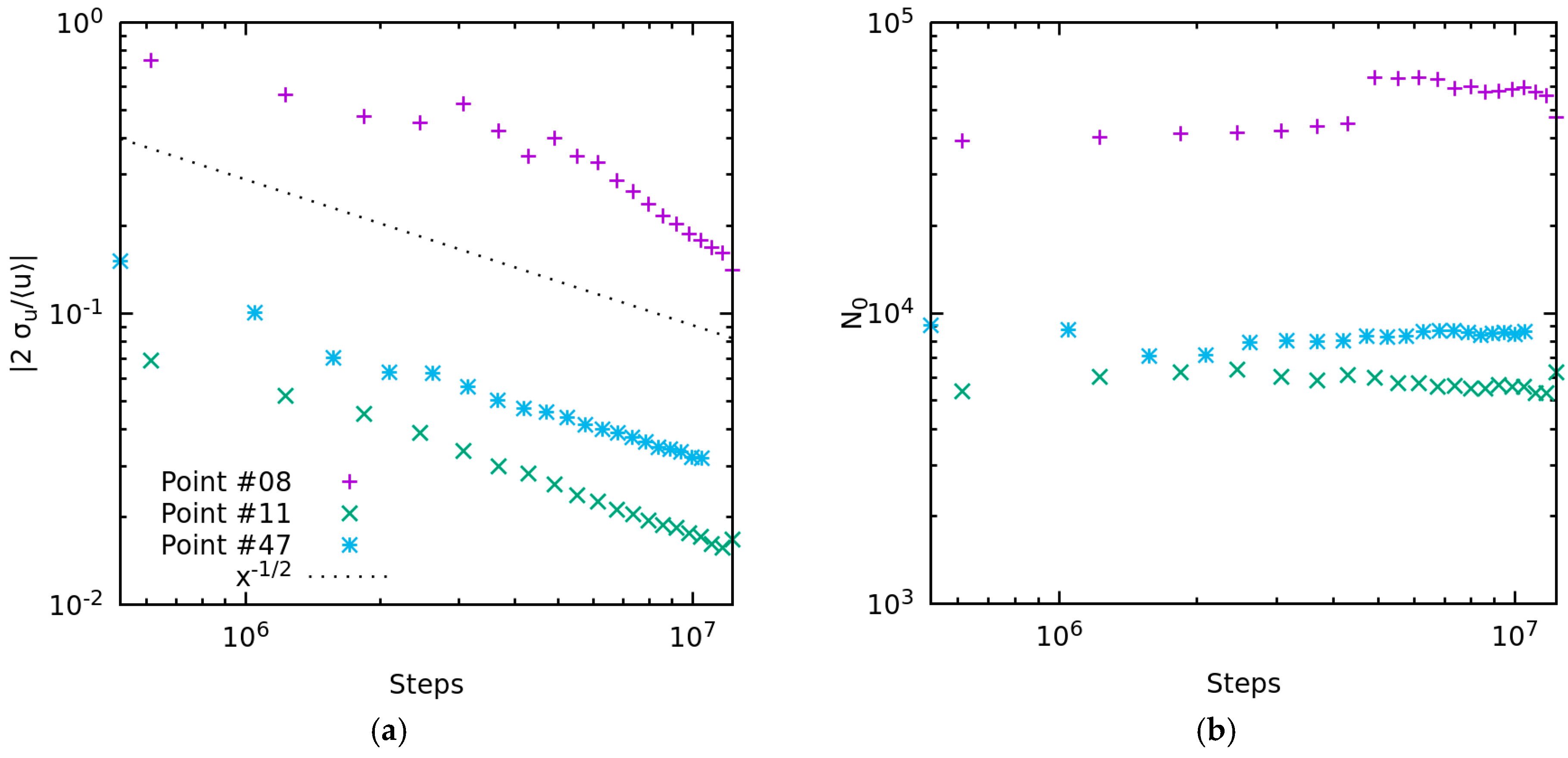
This is also confirmed in the simulation and can be observed in Figure 4, where the convergence of relative 2 σ uncertainty for the streamwise velocity component with number of steps is shown. The figure was produced by calculating the average and the uncertainty approximately every 5 × 10 4 time steps. However, not every time sample was used in the calculation. The data set was down sampled to include every tenth time step. As we show later, this does not have a significant effect on the estimation of uncertainty. The figure also shows convergence of the decorrelation time T 0 , or rather the number of time steps N 0 associated with it.

3.2.1. Uncertainties in Profiles of BFS Results

The uncertainties in monitor points can be overlaid with the profiles that were presented in [1]. The monitor point data cannot be extended to an arbitrary position in space, however, the profile data can be interpolated to the position of the monitor point. In our case, this interpolation was performed in the spectral space. First, we identify the relevant elements in the domain in which the interpolated results are desired. Then, within the elements, which are relevant, the solution in collocation points is transformed into the factors of spectral modes. The appropriate one-dimensional base functions in case of nek5000 are P n ( x ) P n 2 ( x ) , where P n ( x ) is a Legendre polynomial of order n . Note that this is not connected with the PN/PN-2 formulation, where the polynomials used for pressure are actually of lower order. The range of the polynomials is limited to the interval [−1,1]. Appropriate translation and scaling has to be performed to obtain the results at the desired location within the element. Since we are using 7 collocation points per direction in each element, the maximal order of base function polynomial is 6. The interpolated data are obtained by evaluating the base function at the desired location within the element and multiplying by appropriate spectral mode factor.
To obtain the appropriate line profile, two coordinates of the monitor point are taken as the desired location of the line profile. The positions along the line are the same as the positions of collocation points in this direction.
The estimation of statistical uncertainties allows us to put error bars on the results of a DNS. The following figures try to demonstrate the uncertainties within the results in profiles. Since in the DNS we are usually concerned with other sources of uncertainty it might be unusual to see significant error bars which originate only from statistical sources.
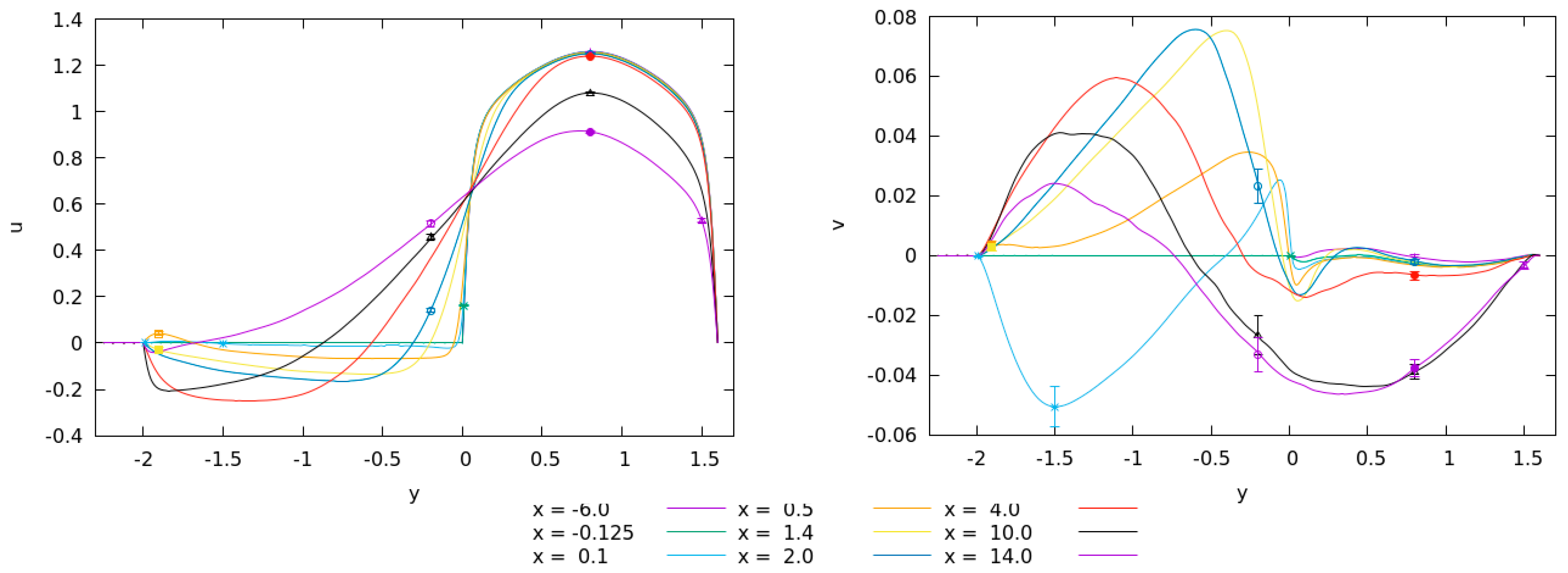
Figure 5 shows the profile lines of average velocity components together with values and 2 σ uncertainties obtained in the relevant monitor points. The profiles are limited to the plane z = 0 , where most of the monitor points lie. However, due to brevity, only some profiles along with appropriate monitor points in this plane are shown. At y < 2 , the heater is present and all velocity values are zero there. For profile x = 0.125 , the region below y < 0 is located inside the step wall and that is why the velocity values are equal to zero.
From the figure it is apparent that the streamwise velocity component is well converged, since the uncertainties are almost invisible. However, for the y velocity component the uncertainties are relatively significant. Also, location significantly influences the uncertainties, if we compare uncertainties at x = 10 and x = 14 . The z component of velocity is the least interesting and is not shown in figure. Although there is a weak flow through the plane z = 0 immediately after the step ( x = 0.1 ), with the added uncertainties it is clear that it is not statistically significant, as is expected due to the symmetry. The average values fall within 2 σ uncertainty of zero.
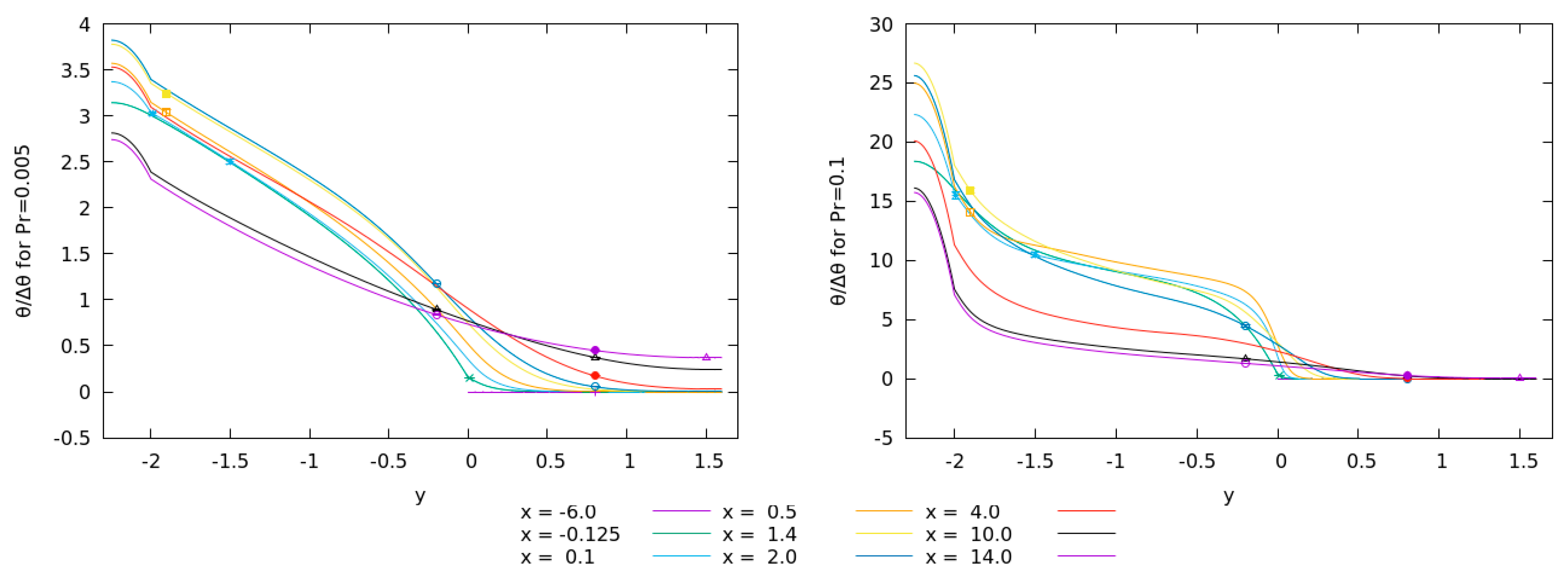
Figure 6 shows the profiles of both passive scalars together with the averages and uncertainties calculated in the monitor points. Here, for the locations at y < 2 the fields are not zero, since the thermal field penetrates into the walls and heater. Similar is true for the location at x = 0.125 and values with y < 0 . The uncertainties in the scalar fields are relatively small, which we attribute to high diffusion due to low Prandtl number.
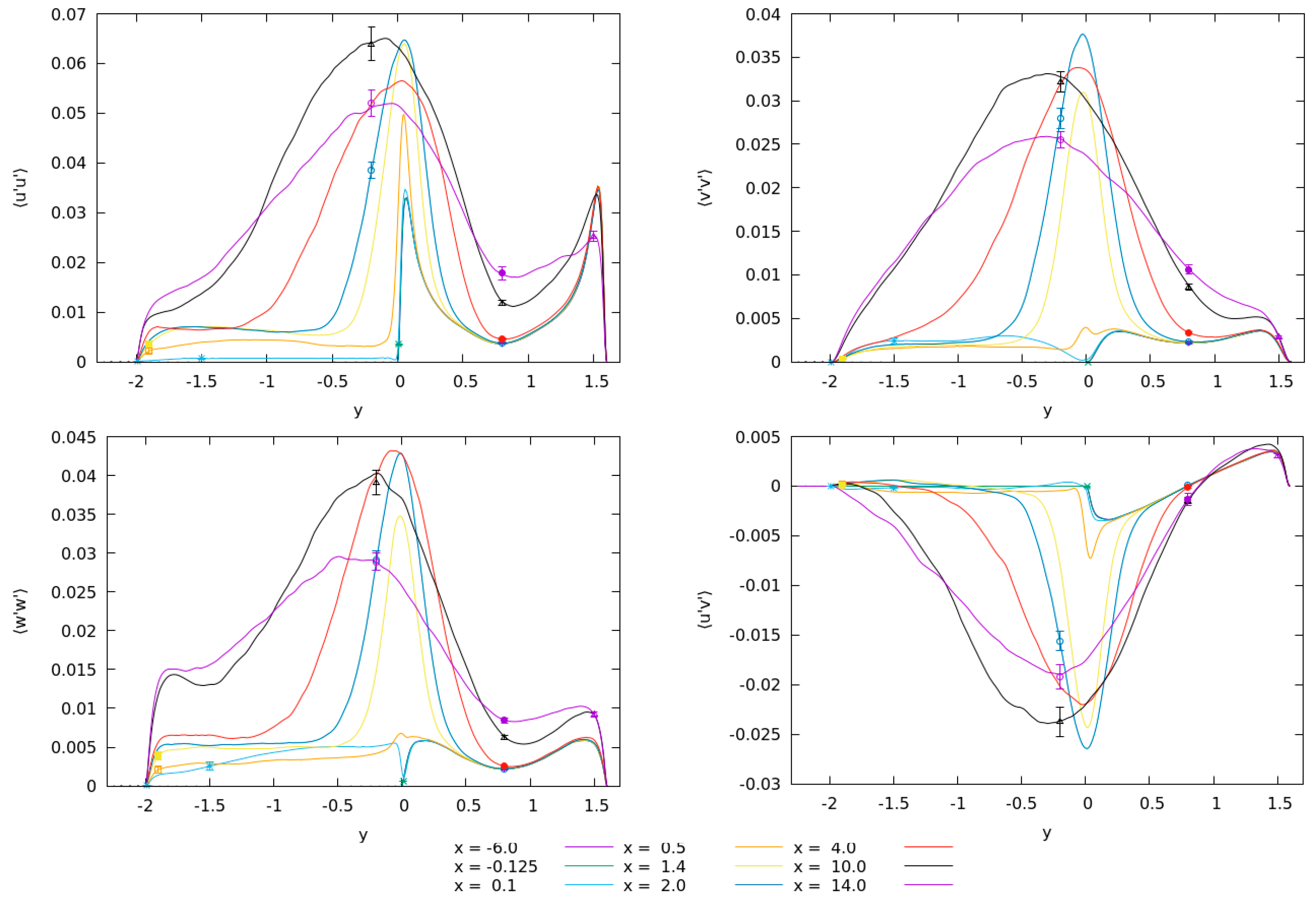
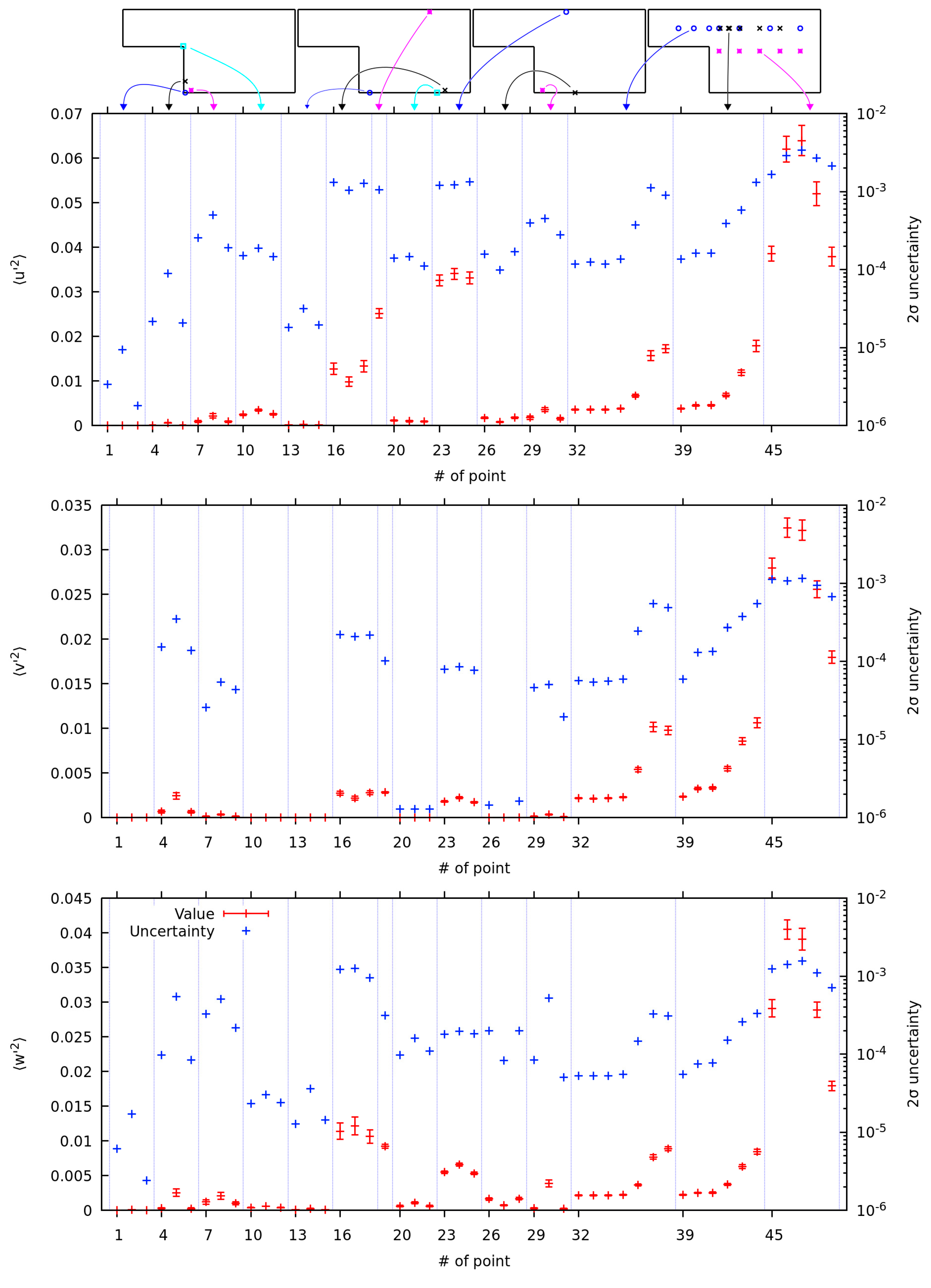
Figure 7 shows the diagonal and non-diagonal components of the Reynolds stress tensor that are expected to be different from zero in the plane z = 0 together with the monitor point data. Some discrepancy between profile and monitor point data can be observed. This is due to data from these particular monitor point was only averaged over around 10 million time steps, while the profile was averaged over 12 million time steps. This is the case for profile of w 2 at x = 10 and monitor point 47 at y = 0.2 .
The averages seem adequately converged and the anisotropy of turbulence immediately after the step is clearly observable (compare profile of fluctuations at x = 0.1 , where fluctuations in x direction are almost twice the fluctuations in y direction). However, this turbulent anisotropy persists towards the outflow (profile and monitor points at x = 10 and x = 14 ). The data from monitor points support the claim that the anisotropy is statistically significant. Of course, the anisotropy of turbulence can also be observed near the walls.
The only non-diagonal component of the Reynolds stress tensor that is non-zero through the plane z = 0 is the u v . At monitor point 48 with x = 14 and y = 0.2 a similar discrepancy can be observed between the profile and the monitor data due to difference in the integration time.
Figure 8 shows the fluctuations of temperature through the middle of the BFS domain. The points located in the stagnation zones and close to the heater exhibit rather high uncertainties in the fluctuations. This is especially apparent in the case of lower Prandtl number. However, our analysis showed that the significant increase of the uncertainties in these regions is more connected to the length of decorrelation time, than to amplitude of oscillations. If we observe the history of temperature fluctuations in various points, it is apparent that at different monitor points the temperature oscillates at different timescales or frequencies. The smoother temperature signals have higher decorrelation times and thus higher uncertainties.
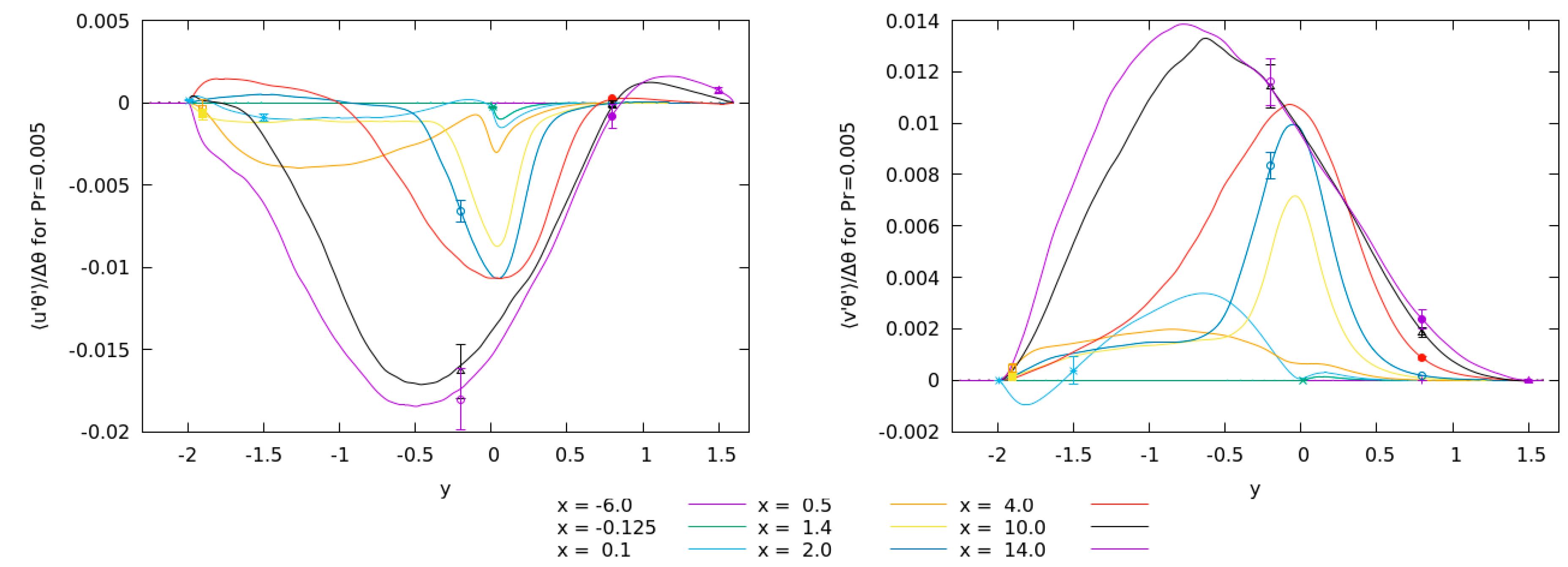
Figure 9 shows the profile of turbulent heat flux components for the passive scalar with Pr = 0.005 through the plane z = 0 . The x and y components of turbulent flux are increasing towards the outflow. The third component is zero within the statistical uncertainty and is not shown.
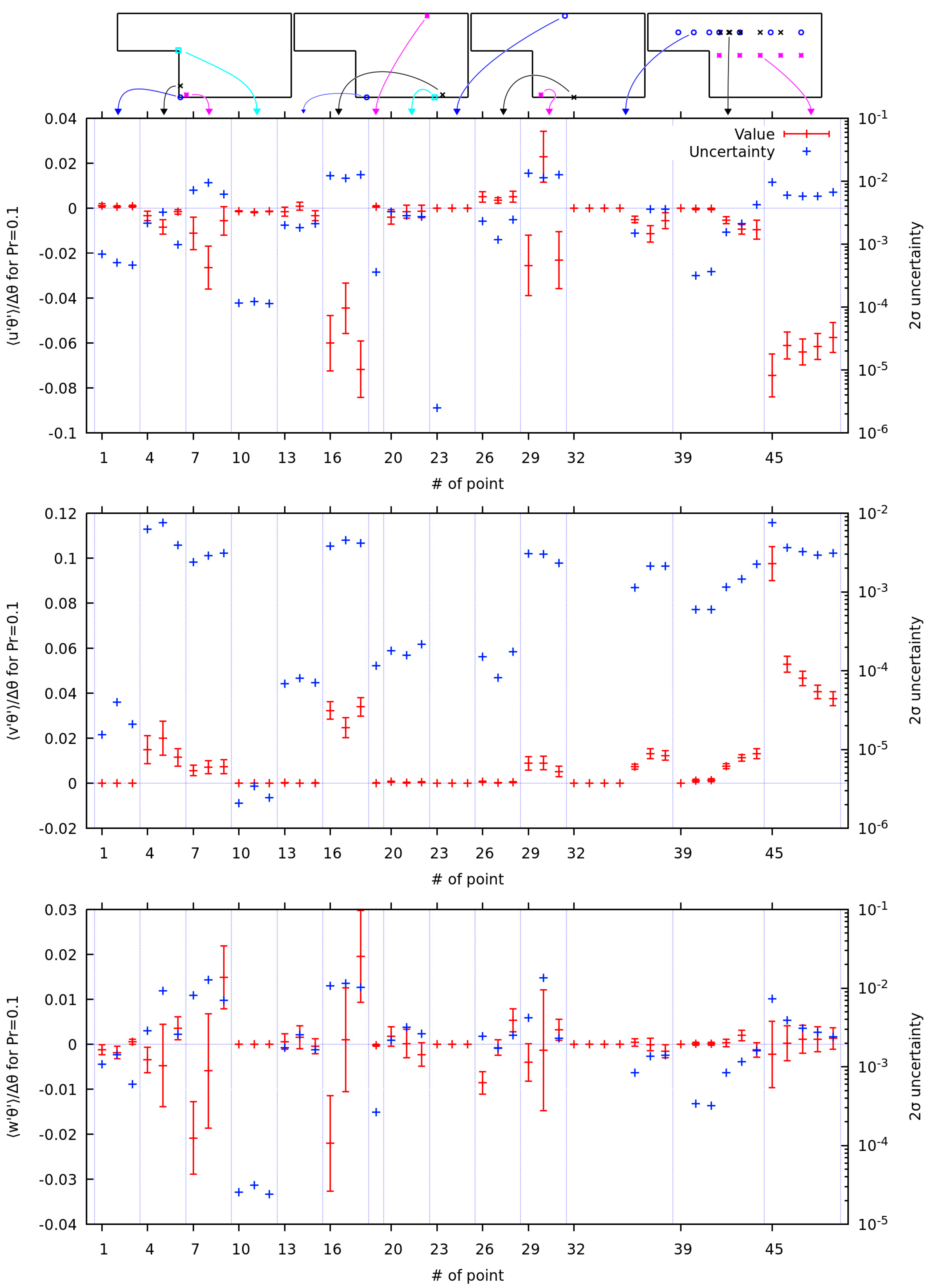
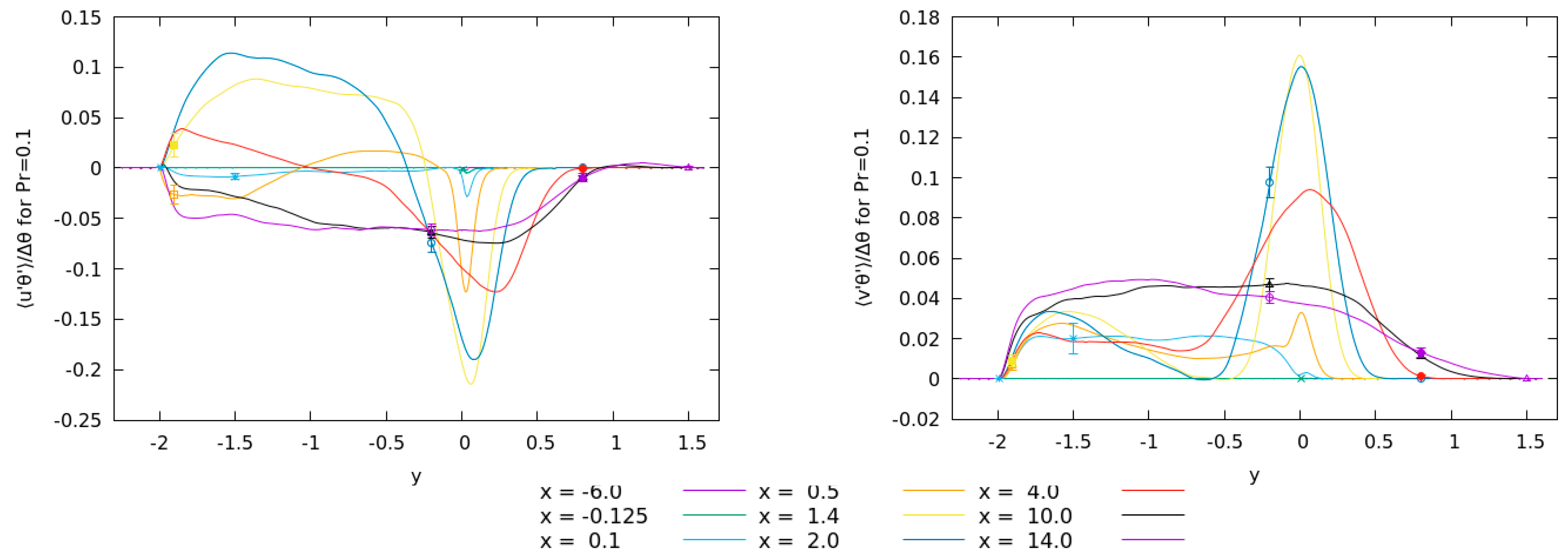
Figure 10 shows the profile of turbulent heat flux for passive scalar with Pr = 0.1 together with values and uncertainties calculated in the monitor points in the plane z = 0 . The x and y components of turbulent heat flux for both Prandtl numbers show that higher uncertainties are found where the average values are higher (unlike with temperature fluctuations above). However, a general observation is that the relative uncertainties in the recirculation zone are a bit higher than outside of it. This is visible with comparison of turbulent heat flux results with similar values, such as v θ component for Pr = 0.005 at points 5 ( x = 0.1 , y = 1.5 , cyan) and 35 ( x = 2 , y = 0.8 , blue) or 41 ( x = 4 , y   = 0.8, red), or component v θ with Pr = 0.1 at points 5 ( x = 0.1 , y = 1.5 , cyan) and 43 ( x = 10 , y = 0.8 , black) or 44 ( x = 14 , y = 0.8, magenta).

3.2.2. Uncertainties in Monitor Points

Figure 11 shows the average velocity components, together with the 2 σ uncertainties, which correspond to roughly 95% confidence interval. The top row shows the approximate position of the appropriate points. This is just a guide for the eye, since point designations are not so informative. The streamwise velocity component shows decent convergence. The relative uncertainty in the average y velocity component seems to be larger, however, this is only because the absolute values of the velocity component are much lower. The absolute uncertainty is actually lower. A similar observation can be made about the z velocity component.
The streamwise velocity component in Figure 11 is mostly positive. Note, however, the points 29 to 31. Since the component changes the sign in these three points, they are located near the stagnation zone. Similarly, the points 20 to 22 lie in a stagnation zone, where the streamwise velocity is close to zero. However, this component has larger absolute value at points 16 to 18 located downstream of the recirculation region and 26 to 28 located in the recirculation region.
The y velocity component at points 16 to 18, 29 to 31, and to a degree in 26 to 28 confirms the structure observed and discussed in [1], where the flow is directed towards the heater at the edges (of z axis) but is directed away from the heater in the middle (around z = 0 ). Also of note is that the velocity component immediately downstream of the step, at points 4 to 6 is directed towards the heater while, for example at point 45, it is directed away from the heater.
Note that values for streamwise and y velocity components should be symmetrical over the plane z = 0 , while the values for the z velocity component should be anti-symmetrical, with values in the plane z = 0 being zero. In fact, such a test can be performed for all the variables shown. Out of 350 such tests that we could perform, 12 tests failed, or around 3.4%. With the above 95% confidence interval, we would expect the failure rate to be around 5%. If such a test is performed with 3 σ uncertainty, only one test fails. At monitor point 43, the z component of turbulent heat flux for passive scalar with Pr = 0.1 is within 4 σ of zero; however, outside of 3 σ range. For 3 σ interval, the confidence interval is around 99.7% and we would expect one test to fail.
The z component of velocity shows the anti-symmetries over the z axis. However, interestingly, the points in the recirculation region have considerably larger uncertainties at z = 0 than at the sides of the domain. This would indicate the flow is fluctuating over this plane, while being more steady at the sides. The only exception seems to be the points 26 to 28 which lie in the recirculation bubble.
Figure 12 shows the diagonal components of Reynolds stress tensor. The uncertainties are comparable between different components, however, the asymmetry of turbulence is still apparent (this is apparent just by observing the scale on the left). The asymmetry can also be found in the statistical uncertainties in the recirculation zone. The turbulent kinetic energy seems to be highest through the middle of the domain. However, there are some exceptions. These are at points 26 to 28, located upstream of the reattachment zone, and at points 16 to 18, located downstream of the reattachment zone. This differs from the reattachment zone, located around points 20 to 22. The peak in fluctuations is found around x = 10 . This is a peculiar result since the flow seems to be more turbulent closer to the lateral walls; however, this is due to the three dimensional structure of the flow. That is, the reattachment does not have a shape of a straight line but is prolonged towards the outflow closer to the lateral walls.
Figure 13 shows the average value, as well as the square of RMS fluctuations for the passive scalar with Pr = 0.005 . The average values have some expected properties: they are higher near the heater and downstream of the step. The drop in temperature through the points 45 to 49 may be surprising; however, fluid from the recirculation zone is heating fluid at points 32 to 38 and 39 to 44. According to the structure of the flow, described in [1] the cold fluid is flowing towards the heater at the sides ( z = ± 1.8 ).
More interesting are the fluctuations of the passive scalar. Immediately one can notice the relatively high uncertainties in fluctuations in points located close to the heater. Unfortunately, no monitor point was placed in the heater to see the behaviour of uncertainties of thermal fluctuations in the solid. Consistently, thermal fluctuations in monitor points located inside or near the recirculation zone show higher statistical uncertainties, compared to thermal fluctuations in monitor points outside of recirculation zone.
Figure 14 shows the similar graph for the passive scalar with Pr = 0.1 . Note that the averaging time here is shorter so we expect slightly higher relative uncertainties. This is the case in the figure, however, we can observe the same trend of uncertainties of thermal fluctuations being higher at the points near the heater. Nevertheless, there are subtle differences, which would indicate that the influence of solid walls in connection with the Prandtl number is stronger than the proximity to the stagnation zones. These differences can be seen in first 6 monitor points 13 to 15, as well as 29 to 31. However, since the lower Prandtl number means wider thermal layer a wider influence of stagnation zones could be observed.
The higher uncertainties in thermal fluctuations, as well as in average values of passive scalars, were traced back to an order of magnitude higher decorrelation times. By Equation (3) this increases the statistical uncertainties. The higher decorrelation time is estimated since the temperature oscillations have longer periods, although the amplitudes of the fluctuations do not seem to be vastly different.
The uncertainties of Reynolds stresses and turbulent heat fluxes can be found in the Appendix A.
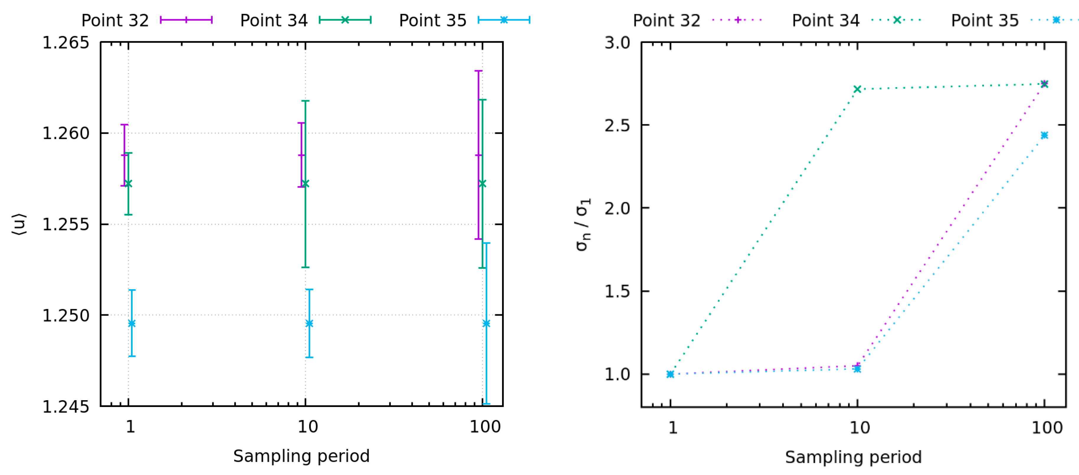
Graphs in Figure 11, Figure 12, Figure 13 and Figure 14 were produced by taking into account monitor data at every time step. An interesting observation can be made if we skip some of the time steps in the calculation of averages. Our time step length was approximately 0.1 of the time step calculated through the Courant–Friedrichs–Lewy condition (CFL time step). We found that the average results do not change by much if values from every hundredth time step (or every tenth CFL time step) are taken. Nevertheless, the uncertainties of these averages can differ by up to a single-digit factor. This results from the different estimation of the decorrelation time T 0 .
It should also be noted that by taking every time step data, the order of the auto-regression model has to be set to very high values to properly estimate the decorrelation time. The order for two variables at point 8 was as high as the maximal order we used, which is around 65,000. For around 8 other variables and points, the estimated order was above 60,000. This increases the demands for memory considerably and slows down the statistical analysis. If the maximal order of the auto-regression model was set to the default value of 512, the results significantly diverged from the proper results and from results where only every tenth or hundredth time step is used for estimation. In the latter two cases the increase of the maximal order of the auto-regression model does not need to be so drastic, since the number of parameters needed to properly determine the autocorrelation function also decreases with down sampling. Our simulation is, therefore, considerably oversampled for determination of the statistical variables with the arsel library.
With all of the above, our conclusion is that the frequency of monitoring data can safely be reduced. Nevertheless, the data from the channel flows suggest that the period of sampling should not pass over 10 CFL time step as there the results start to differ significantly. A similar effect is observed in the BFS flow and is shown in Figure 15 for three points. Although other variables and other monitor points also show some changes, we selected the streamwise velocity component and in points where the changes are among the greatest. Note, however, that the average value itself changed insignificantly. The only change is in the estimated uncertainty of the averages.
3.3. A Priori Estimation of the Statistical Uncertainty

For both cases considered here, one can estimate the order of magnitude of the statistical uncertainty plaguing the averaged velocity prior to the DNS. A coarse estimation of the correlation time T 0 can be obtained from a characteristic length L and velocity scale: T 0 = L / u . Then, assuming a given turbulence intensity I = k / u , one can compute the relative statistical uncertainty for the averaged velocity corresponding to a given simulation time T :
2 σ u 2 u k T T 0 1 .
For the channel flow case, using wall-units, u is around 10, L is around 180 (in wall units) and the turbulent kinetic energy per unit mass is around 10. This leads to a decorrelation time T 0 of around 18. The simulations time is around 54 thousand. The corresponding relative statistical error without spatial averaging is around 1.1 %, which is the order of magnitude observed in the top-left frame of Figure 3.
For the BFS case, after the step, u is around 0.6, L is around 3.6 and the turbulent kinetic energy per unit mass is around 0.01. This leads to a decorrelation time T 0 of around 6. The simulation time is around 4800. The corresponding relative statistical error is around 1.2 %, which is in the same order of magnitude observed in the top frame of Figure 11.
Using the correlation time associated with the averaged velocity, one can compute the relative statistical uncertainty for the average temperature from I = θ 2 / θ . For both passive scalars in the BFS configuration, I is around 0.1, θ / Δ θ is around 1 and 10, θ 2 / ( Δ θ ) 2 is around 0.01 and 1, and the relative statistical uncertainty on the averaged velocity is around 0.7 %, which is in the same order of magnitude observed in the top frame of Figure 13 and Figure 14.
Indeed, the proposed estimators only provide an order of magnitude for the relative statistical error on the averaged velocity and temperature: the actual correlation time is not constant across the domain and might even change depending on the velocity component considered. However, the authors conjecture that the estimator can be combined with a RANS simulation, from which both k , θ 2 , u and θ can be obtained. The estimator defines the lower limit for uncertainty of RANS simulation due to the turbulent nature of the flow. Although RANS simulation results are burdened with other sources of error, which are usually of greater concern, this might provide an accurate a-priori estimator for the DNS, LES or unsteady RANS simulation and averaging times needed to obtain a given statistical error on the averaged velocity. If the RANS simulation could provide an estimation of the variance of the temperature, one could also build an estimator for the relative statistical error plaguing the averaged temperature. Of course, once a DNS or LES is already running, the estimate of the needed averaging time can be obtained with the arsel toolchain.

4. Conclusions

We presented uncertainties of statistical quantities obtained in the DNS of channel flow, and of flow in a BFS. While the channel flow uncertainties are below a few percent, the uncertainties in the BFS at certain positions become higher. The highest relative uncertainties in the case of BFS are found near the stagnation zones, where velocities are low. As we have shown, spatial averaging can significantly reduce absolute statistical uncertainties. In case of channel flow, this is also carried over to relative statistical uncertainties.
The uncertainty of individual components of average velocity, Reynolds stress tensor, average temperature, as well as the turbulent heat flux in case of BFS follows similar patterns as in the case of channel flow. The temperature fluctuations in the case of BFS show higher uncertainties in the recirculation region and close to the heat source.
We provide a general estimator for statistical uncertainty of average velocity and temperature. Since it uses turbulence kinetic energy, temperature variance, average velocity and temperature, the estimator can be used to evaluate lower bound of the uncertainties of average velocity results in RANS simulations. Nevertheless, with an appropriate estimation of the decorrelation time of other variables, such as Reynolds stresses, the estimator could be used to predict relative uncertainties of that variable. For the DNS simulation, the estimator can be used to predict the averaging time needed for uncertainty to drop to required levels. Of course, this recommendation must be understood in a general way, since at some locations, the expected value of a velocity component might be zero and relative statistical uncertainty is meaningless at such points.
We also observed that not every data sample from every time step is needed to produce accurate averages. The averages are accurate even if one includes only samples from every first or even tenth duration of the CFL time step. Obviously, the CFL time step is defined globally, for the whole domain. However, locally this period might even increase. Nevertheless, for accuracy of the uncertainty, we noticed that different periods of sampling could produce more discrepancies. Approximately by a factor of 2 or 3.

Author Contributions

Conceptualization, I.T., C.F., J.O.; methodology, C.F., I.T., J.O.; simulation of channel flow, I.T.; BFS simulation, J.O.; writing—original draft preparation, J.O.; writing—review and editing, I.T., C.F.; visualization, J.O.; supervision, I.T.; project administration, I.T.; funding acquisition, I.T. All authors have read and agreed to the published version of the manuscript.

Funding

This research was funded by Slovenian Research Agency, grants P2-0026 and L2-9210. Research is part of the SESAME project funded by the EURATOM Research and Training Programme (#654935) of the European Commission (H2020).

Institutional Review Board Statement

Not applicable.

Informed Consent Statement

Not applicable.

Data Availability Statement

Data from this article is available upon request to the corresponding author.

Conflicts of Interest

The authors declare no conflict of interest.

Nomenclature

DNSDirect Numerical Simulation
BFSBackward Facing Step
RMSRoot-mean-square
Pr Prandtl number
Re Reynolds number
T , N = T / Δ t Integration time, number of time steps used for averaging
T 0 , N 0 = T 0 / Δ t Decorrelation time, number of time steps between decorrelated samples
Δ t Time between two consecutive time steps
u , v , w Velocity components in direction x , y and z , respectively
σ Statistical uncertainty of a variable
Δ θ Increase of temperature θ of a perfectly mixed fluid from inflow to outflow
a Average value of variable a
a Fluctuating part of variable a , that is a = a a

Appendix A

Positions of monitor points in the BFS case are given in Table A1.
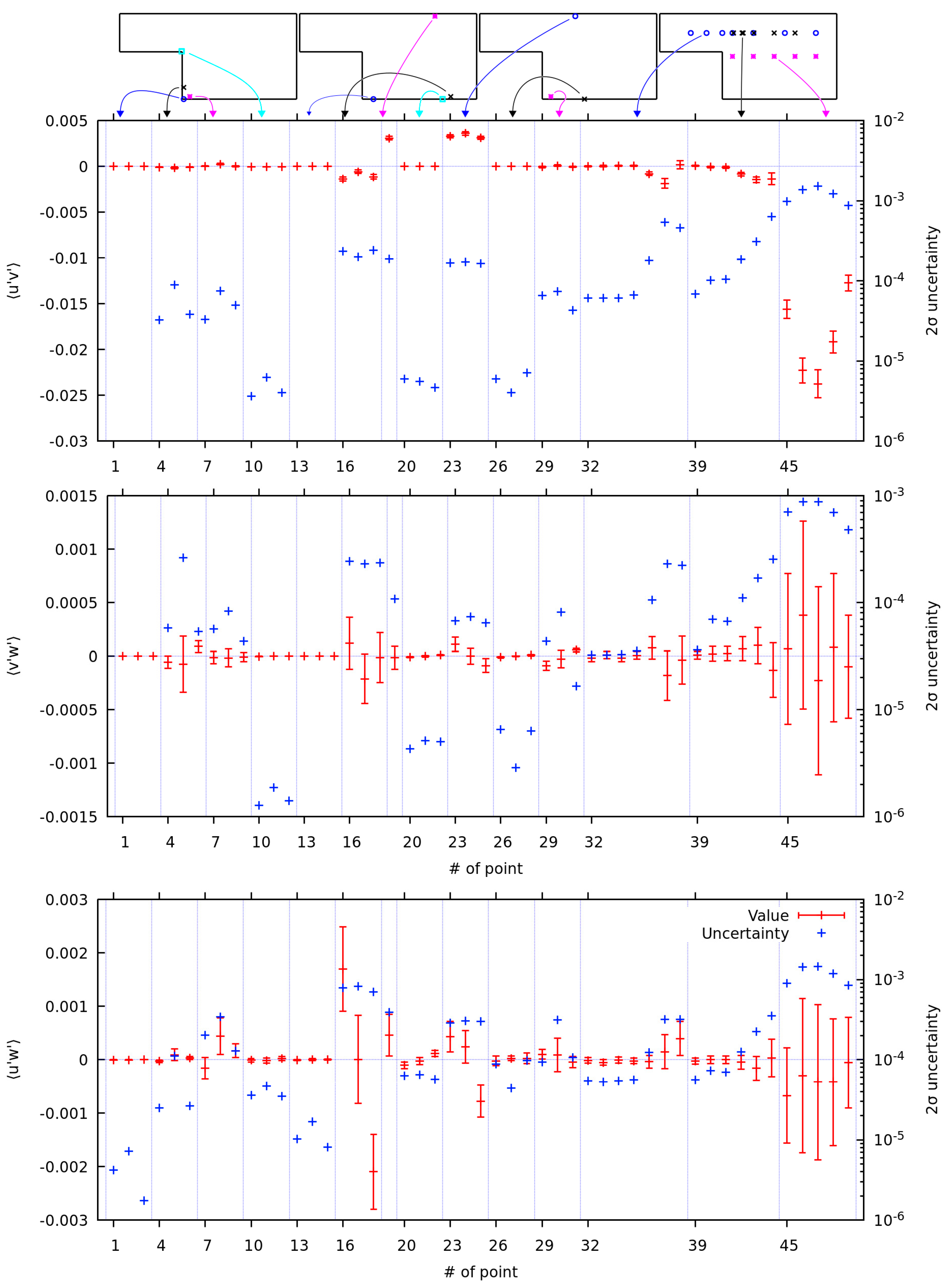
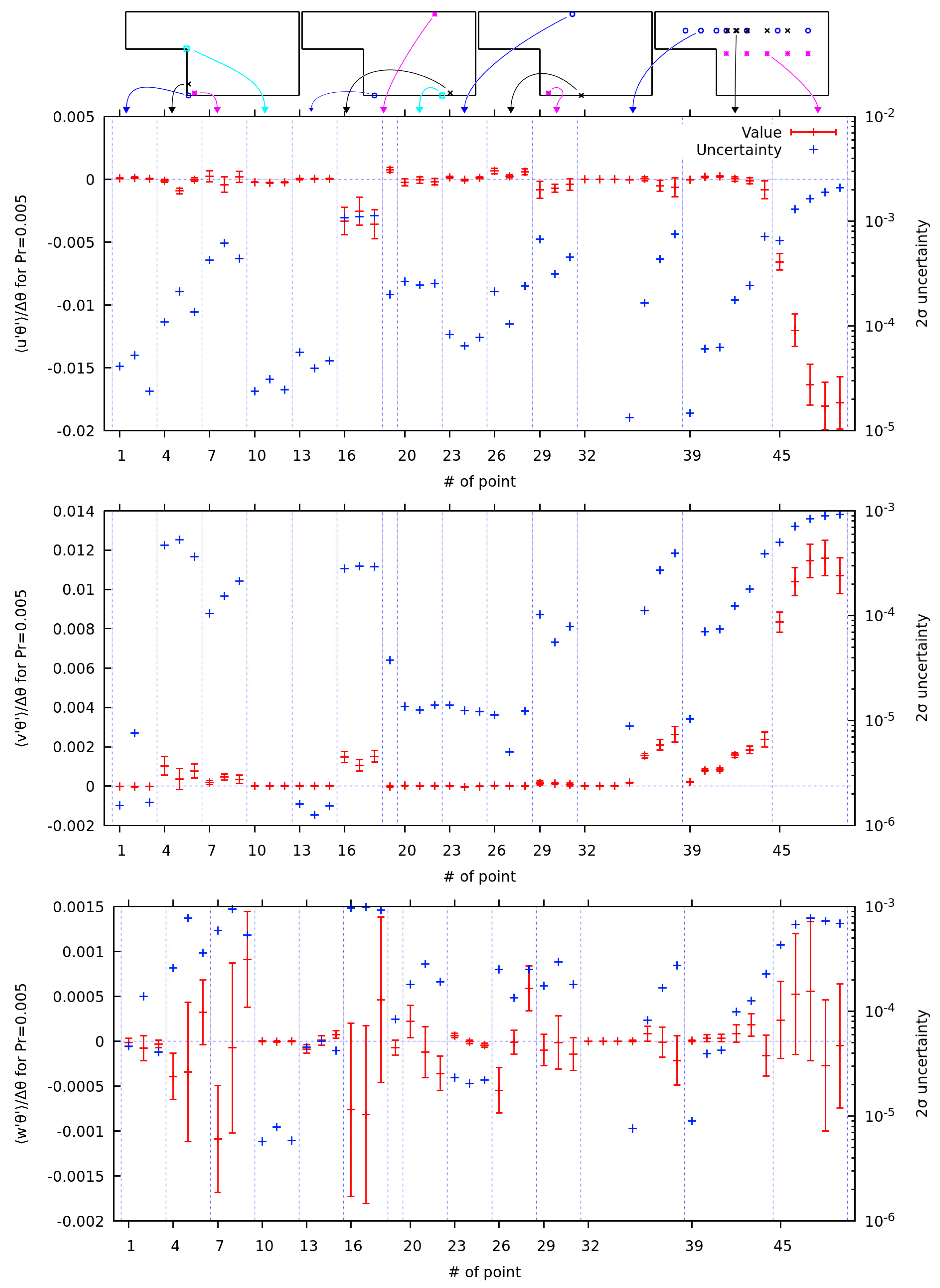
Figure A1 shows the non-diagonal components of Reynolds stress. As indicated in Section 3.2.1, only the component u v has non-zero components in the plane z = 0 . Nevertheless, at some monitor points we can observe that the other two components have average values that are beyond 2 σ distance away from zero in the plane z = 0 (point 8). As noted before, some discrepancies are expected due to the limited confidence range. The relative uncertainties for the two other non-diagonal components of Reynolds stress seem high; however, since the averages are expected to be zero, the relative uncertainties explode, even though they are comparable with component u v . The other two components do have non-zero components in other planes. In the monitor points that are chosen symmetrically over the plane z = 0 , the values are expected to be symmetrical too. Note that components involving the w component of velocity are expected to be anti-symmetric. These tests were included in the aforementioned 350 tests of which 3.4% failed.
Figure A2 shows the components of turbulent heat flux for passive scalar with Pr = 0.005 and Figure A3 shows the components of turbulent heat flux for passive scalar with Pr = 0.1 . As with the non-diagonal components of Reynolds stresses, we expect that components involving w component of velocity are anti-symmetric in symmetrically chosen monitor points and zero in monitor points through the plane z = 0 . Other components of turbulent heat flux are expected to be symmetrical in symmetrically chosen monitor points.
Table A1. Positions of the monitor points throughout the domain.
Point x y z
10.1−1.99−1.6
20.1−1.990
30.1−1.991.6
40.1−1.5−1.6
50.1−1.50
60.1−1.51.6
70.5−1.9−1.2
80.5−1.90
90.5−1.91.2
10−0.1250.01−1.2
11−0.1250.010
12−0.1250.011.2
132.2−1.99−1.2
142.2−1.990
152.2−1.991.2
1617−1.9−0.9
1717−1.90
1817−1.90.9
19141.50
2015.5−1.99−1.6
2115.5−1.990
2215.5−1.991.6
236.41.5−1.2
246.41.50
256.41.51.2
268.1−1.99−1.2
278.1−1.990
288.1−1.991.2
291.4−1.9−1.6
301.4−1.90
311.4−1.91.6
32−60.80
33−30.80
3400.80
3520.80
3660.80
37120.80
38180.80
392.1250.80
403.8750.80
4140.80
426.1250.80
43100.80
44140.80
452−0.20
466−0.20
4710−0.20
4814−0.20
4918−0.20
Figure A1. x -axis: number of point according to Figure 2. Top to bottom: Reynolds stress components u v , v w and u w . Red dots represent root-mean-square values with ±   2 σ range (left scale), green dots represent ( 2 σ ) uncertainty (right scale).
Applsci 11 01399 g0a1
Figure A2. x -axis: number of point according to Figure 2. Top to bottom: turbulent heat flux components for Pr = 0.005 : u θ , v θ and w θ . Red dots represent root-mean-square values with ±   2 σ range (left scale), green dots represent ( 2 σ ) uncertainty (right scale).
Applsci 11 01399 g0a2
Figure A3. x -axis: number of point according to Figure 2. Top to bottom: turbulent heat flux components for Pr = 0.1 : u θ , v θ and w θ . Red dots represent root-mean-square values with ±   2 σ range (left scale), green dots represent ( 2 σ ) uncertainty (right scale).
Applsci 11 01399 g0a3

References

  1. Oder, J.; Shams, A.; Cizelj, L.; Tiselj, I. Direct numerical simulation of low-prandtl fluid flow over a confined backward facing step. Int. J. Heat Mass Transf. 2019, 142, 118436. [Google Scholar] [CrossRef]
  2. Oliver, T.A.; Malaya, N.; Ulerich, R.; Moser, R.D. Estimating uncertainties in statistics computed from direct numerical simulation. Phys. Fluids 2014, 26, 035101. [Google Scholar] [CrossRef] [Green Version]
  3. Pope, S.B. Turbulent Flows; Cambridge University Press: Cambridge, UK, 2011. [Google Scholar]
  4. Vreman, A.W.; Kuerten, J.G.M. Comparison of direct numerical simulation databases of turbulent channel flow at reτ= 180. Phys. Fluids 2014, 26, 015102. [Google Scholar] [CrossRef] [Green Version]
  5. Vinuesa, R.; Prus, C.; Schlatter, P.; Nagib, H.M. Convergence of numerical simulations of turbulent wall-bounded flows and mean cross-flow structure of rectangular ducts. Meccanica 2016, 51, 3025–3042. [Google Scholar] [CrossRef] [Green Version]
  6. Ries, F.; Nishad, K.; Dressler, L.; Janicka, J.; Sadiki, A. Evaluating large eddy simulation results based on error analysis. Theor. Comput. Fluid Dyn. 2018, 32, 733–752. [Google Scholar] [CrossRef] [Green Version]
  7. Andrade, J.R.; Martins, R.S.; Thompson, R.L.; Mompean, G.; da Silveira Neto, A. Analysis of uncertainties and convergence of the statistical quantities in turbulent wall-bounded flows by means of a physically based criterion. Phys. Fluids 2018, 30, 045106. [Google Scholar] [CrossRef]
  8. Tiselj, I.; Bergant, R.; Mavko, B.; Bajsic´, I.; Hetsroni, G. Dns of turbulent heat transfer in channel flow with heat conduction in the solid wall. J. Heat Transf. 2001, 123, 849–857. [Google Scholar] [CrossRef]
  9. Oder, J. Direct Numerical Simulation of Flow Seaparation with Heat Conduction. Ph.D. Thesis, University of Ljubljana, Ljubljana, Slovenia, 2019. [Google Scholar]
  10. Oder, J.; Tiselj, I.; Jäger, W.; Schaub, T.; Hering, W.; Otic, I.; Shams, A. Thermal fluctuations in low-prandtl number fluid flows over a backward facing step. Nucl. Eng. Des. 2020, 359. [Google Scholar] [CrossRef]
  11. Kawamura, H.; Ohsaka, K.; Abe, H.; Yamamoto, K. Dns of turbulent heat transfer in channel flow with low to medium-high prandtl number fluid. Int. J. Heat Fluid Flow 1998, 19, 482–491. [Google Scholar] [CrossRef]
  12. Gavrilakis, S.; Tsai, H.M.; Voke, P.R.; Leslie, D.C. Direct and Large Eddy Simulation of Turbulence, Notes on Numerical Fluid Mechanics Vol.; Schumann, U., Friedrich, R., Eds.; DBR: Braunschweig, Germany, 1986; Volume 105, p. 410. [Google Scholar]
  13. Lam, K.; Banerjee, S. Investigation of Turbulent Flow Bounded by a Wall and a Free Surface; Invited paper; American Society of Mechanical Engineers, Fluids Engineering: New York, NY, USA, 1988; pp. 29–38. [Google Scholar]
  14. Tiselj, I.; Pogrebnyak, E.; Li, C.; Mosyak, A.; Hetsroni, G. Effect of wall boundary condition on scalar transfer in a fully developed turbulent flume. Phys. Fluids 2001, 13, 1028–1039. [Google Scholar] [CrossRef]
  15. Tiselj, I.; Cizelj, L. Dns of turbulent channel flow with conjugate heat transfer at prandtl number 0.01. Nucl. Eng. Des. 2012, 253, 153–160. [Google Scholar] [CrossRef]
  16. Tiselj, I. Tracking of large-scale structures in turbulent channel with direct numerical simulation of low prandtl number passive scalar. Phys. Fluids 2014, 26. [Google Scholar] [CrossRef]
  17. Niemann, M.; Fröhlich, J. Buoyancy-affected backward-facing step flow with heat transfer at low prandtl number. Int. J. Heat Mass Transf. 2016, 101, 1237–1250. [Google Scholar] [CrossRef]
  18. Flageul, C.; Tiselj, I. Letter: Convergence rate of individual and global quantities in direct numerical simulations. Phys. Fluids 2018, 30, 111704. [Google Scholar] [CrossRef] [Green Version]
Figure 1. Sketch of backward-facing step (BFS) domain used in the direct numerical simulation (DNS). Flow flows from the narrow end towards the wide end. The blue and red coloured blocks are solid walls. Except for the inflow and outflow, all other surfaces are no-slip velocity boundary conditions.
Applsci 11 01399 g001
Figure 2. Distribution of points as seen from positive z axis.
Applsci 11 01399 g002
Figure 3. Various turbulence statistics (sloid lines, left scale) in channel flow with uncertainties (symbols; right scale).
Applsci 11 01399 g003
Figure 4. Convergence of relative 2 σ uncertainty of average streamwise component in three monitor points (a) and convergence of the decorrelation time expressed as number of time steps (b).
Applsci 11 01399 g004
Figure 5. Selected profiles of average velocity components through the midplane ( z = 0 ) at positions where monitor points are present together with the 2 σ uncertainty in these points.
Applsci 11 01399 g005
Figure 6. Passive scalar profiles together with monitor point data uncertainties at specific positions in the plane z = 0 .
Applsci 11 01399 g006
Figure 7. Profile of non-zero components of the Reynolds stress tensor at certain positions in the plane z = 0 .
Applsci 11 01399 g007
Figure 8. Temperature fluctuations for both passive scalars with data from monitor points in the plane z = 0 .
Applsci 11 01399 g008
Figure 9. Profile of turbulent heat flux components for passive scalar with Pr = 0.005 , together with values and uncertainties calculated in monitor points in the plane z = 0 .
Applsci 11 01399 g009
Figure 10. Profile of turbulent heat flux components for passive scalar with Pr = 0.1 toghether with values and uncertainties calculated in monitor points through the plane z = 0 .
Applsci 11 01399 g010
Figure 11. x -axis: number of point according to Figure 2. Top: Mean x -direction velocity. Middle: y -direction velocity. Bottom: z -direction velocity. Red dots represent average values with ±   2 σ range (left scale), blue dots represent ( 2 σ ) uncertainty (right scale).
Applsci 11 01399 g011
Figure 12. x -axis: number of point according to Figure 2. Top: Fluctuations of x -direction velocity. Middle: Fluctuations of y -direction velocity. Bottom: z -direction velocity. Red dots represent root-mean-square values with ±   2 σ range (left scale), blue dots represent ( 2 σ ) uncertainty (right scale).
Applsci 11 01399 g012
Figure 13. x -axis: number of point according to Figure 2. Top: Mean temperature for Pr = 0.005 . Bottom: θ 2 / Δ θ 2 for Pr = 0.005 . Red dots represent root-mean-square values with ±   2 σ range (left scale), blue dots represent ( 2 σ ) uncertainty (right scale).
Applsci 11 01399 g013
Figure 14. x -axis: number of point according to Figure 2. Top: Mean temperature for Pr = 0.1 . Bottom: θ RMS for Pr = 0.1 . Red dots represent root-mean-square values with ±   2 σ range (left scale), blue dots represent ( 2 σ ) uncertainty (right scale).
Applsci 11 01399 g014
Figure 15. Comparison of results with different sampling periods. On the left, the average streamwise velocity component in three points together with the 2 σ uncertainty is shown. On the right, the uncertainty change with sampling rate for the same three points is shown.
Applsci 11 01399 g015
Table 1. Number of time steps used for integration.
DescriptionPointsMonitor Points/Millions of Time StepsProfile Data/Millions of Time Steps
Velocity ,   pressure ,   passive   scalar   with   Pr = 0.005 1–311212
Velocity ,   pressure ,   passive   scalar   with   Pr = 0.005 32–491012
Passive   scalar   Pr = 0.1 1–4977
Publisher’s Note: MDPI stays neutral with regard to jurisdictional claims in published maps and institutional affiliations.