Microseismic Location Error Due to Eikonal Traveltime Calculation

Abstract

The accuracy of computed traveltimes in a velocity model plays a crucial role in localization of microseismic events. The conventional approach usually utilizes robust fast sweeping or fast marching methods to solve the eikonal equation numerically with a finite-difference scheme. These methods introduce traveltime errors that strongly depend on the direction of wave propagation. Such error results in moveout changes of the computed traveltimes and introduces significant location bias. The issue can be addressed by using a finite-difference scheme to solve the factored eikonal equation. This equation yields significantly more accurate traveltimes and therefore reduces location error, though the traveltimes computed with the factored eikonal equation still contain small errors with systematic bias. Alternatively, the traveltimes can be computed using a physics-informed neural network solver, which yields more randomized traveltimes and resulting location errors.

1. Introduction

Diffraction stacking is a recently developed method for locating microseismic events. The method utilizes hodographs from every grid point of a selected volume to build an image function through stacking recorded waveforms along this hodograph [1]. When a grid point coincides with the event location and other imaging conditions are properly applied, the stack will produce a maximum value due to constructive interference indicating the location of the event (e.g., [2]). Diffraction stacking, therefore, requires accurate traveltimes between receivers and potential locations. The errors in traveltime computation will propagate into the stack and result in inaccurate event locations. It is known that errors in surface monitoring mainly result in mispositioning in depth as the depth trades off with origin time (e.g., [3]). Generally, we must conclude that an event will be located inaccurately. One of the efficient and popular approaches of computing traveltimes is solving the eikonal equation using an iterative fast sweeping method (FSM) [4] or direct fast marching method (FMM) [5]. However, a simple discretization of the eikonal equation yields inaccurate solution due to the singularity at the point-source. Since the wavefront curvature around the point-source is extremely large, the finite-difference approximation results in large truncation errors that propagate into the entire computational domain [4]. While it is often mentioned that the maximal errors occur along the diagonal directions from the source, authors typically utilize the $L^1$, $L^2$ or $L^{\infty }$ norm to estimate traveltime error for the entire model volume (e.g., [6,7]).

In this paper, we illustrate the effect of this discretization error in the context of microseismic monitoring from surface arrays and show that the first-order discretization scheme of FSM creates a location bias due to the strong offset dependence of the traveltime errors. We compare location errors resulting from traveltime computation using the original FSM [4], the factored FSM [8], and a recently proposed algorithm for solving the eikonal equation using physics-informed neural networks (PINNs) [9]. We observe large traveltime errors for the original FSM resulting in significantly inaccurate locations of microseismic events. However, the other two approaches yield highly accurate traveltimes, leading to acceptable location errors due to traveltime computation. By using transfer learning, a machine learning technique that relies on storing knowledge gained while solving one problem and applying it to a different but related problem, we observe that computations using PINNs can be accelerated significantly.

2. Methods

2.1. Diffraction Stacking

First, we briefly review diffraction stacking—the preferred industrial methodology for surface monitoring technique used for detection and localization of microearthquakes from dense arrays (hundreds to thousands of receivers) [1]. At the initial step, we select a volume of interest, which coincides with the zone of expected microseismic activity. We discretize the volume and consider each grid node to be a potential source position. Then for each point $\mathbf{x}$ we compute P-wave traveltimes $T_R\left(\mathbf{x}\right)$ for the given velocity model as if this point was a microseismic event. Since the origin time of events is unknown, we also consider all possible values of origin time t. After stacking amplitudes of all M receivers (typically vertical component only) along the predicted hodographs $T_R\left(\mathbf{x}\right)$ we obtain a 4D image function:

$$F(\mathbf{x},t)=\left|\sum _{R=1}^M{\varphi }_R\left(\mathbf{x}\right)A_R(t+T_R\left(\mathbf{x}\right))\right|.$$

(1)

In order to account for the source radiation pattern and ensure constructive interference of signals with reversed polarities, we introduce an amplitude sign correction ${\varphi }_R\left(\mathbf{x}\right)$, which is equal to +1 or $-1$. At every 4D point $(\mathbf{x},t)$, we use least-squares inversion to estimate the moment tensor based on the distribution of the summed amplitudes $A_R(t+T_R\left(\mathbf{x}\right))$ across all receivers, evaluate the weights ${\varphi }_R\left(\mathbf{x}\right)$ for each receiver, and correct for the source mechanism prior to stacking.

If a microseismic event has sufficiently strong signal, it will create a local maximum of the image function in space and time. When velocity model is correct and the traveltimes are computed accurately, this maximum is at the true location and origin time of the microseismic event. In real life application, the velocity model normally introduces location errors, since it always describes only some approximation of elastic properties of the subsurface. Since in this work we are interested in location errors caused by incorrect traveltime computations, in the examples section we consider only rather simple synthetic models in order to exclude other factors affecting location accuracy.

2.2. FSM for the Eikonal Equation

We begin by reviewing the first order fast-sweeping method for the eikonal equation. Let us consider the isotropic eikonal equation:

$${|\nabla T|}^2=S^2\left(\mathbf{x}\right),$$

(2)

where T is the traveltime, $S\left(\mathbf{x}\right)$ is the slowness of the medium and $|·|$ is the Euclidean norm. This equation can be effectively solved numerically using the so called upwind discretization scheme [10]. In the 3D case, for each grid point $\mathbf{C}$, we need to consider eight tetrahedrons (Figure 1) and solve the discretized eikonal equation:

$$|(T_C-T_w,T_C-T_S,T_C-T_D){|}^2=h^2{S}^2\left(\mathbf{C}\right),$$

(3)

where h is the grid interval that we assume to be the same in all three directions for simplicity. The value of $T_C$ can be found from this quadratic equation and should be tested for causality: $T_C$ must be larger than time values $T_W$, $T_S$, $T_D$ in all three neighboring grid points used in Equation (3). In cases when the causality condition is violated, Equation (3) should be reduced to the 2D case and solved similarly for each triangular face of the selected tetrahedron ($\Delta CWD$, $\Delta CSD$, $\Delta CWS$). This happens when the normal to the wavefront is parallel to one of the coordinate planes $XY$, $XZ$, or $YZ$. When the equation does not have a causal solution in the 2D case as well, the solution is propagated along the edges of corresponding triangle. For example, in case of triangle $\Delta CWD$, the candidates for traveltime values for $T_C$ are $T_W+hS\left(\mathbf{C}\right)$ and $T_D+hS\left(\mathbf{C}\right)$. Finally, in such cases, the $T_C$ value is determined as minimum of all candidates computed for all eight tetrahedrons, and this value is used to update traveltime value in the grid point $\mathbf{C}$.

After initialization of the traveltime volume by assigning zero at the source location and a large value at all other points, the algorithm calculates traveltimes for all the points in the domain in eight alternating orders, “sweeping” the whole volume several times to evaluate all directions of the propagating waves. With I, J, and K being a number of points in the X, Y, and Z directions, respectively, theses sweeping orders can be written in the following form:

$$\begin{array}{c}\hfill i=1:I,j=1:J,k=1:K\\ \hfill i=1:I,j=J:1,k=1:K\\ \hfill i=I:1,j=1:J,k=1:K\\ \hfill i=I:1,j=J:1,k=1:K\\ \hfill i=1:I,j=1:J,k=K:1\\ \hfill i=1:I,j=J:1,k=K:1\\ \hfill i=I:1,j=1:J,k=K:1\\ \hfill i=I:1,j=J:1,k=K:1\end{array}$$

Here i, j, and k are grid point indices in X, Y, and Z directions, respectively. The method is robust and easy to implement; however, due to the singularity at the source position (and any other point where wavefront significantly curves), the solution inevitably accumulates errors. It is known that the largest error appears in the diagonal directions [4]. As we will show in the examples section, this can be critical for the purposes of microseismic imaging.

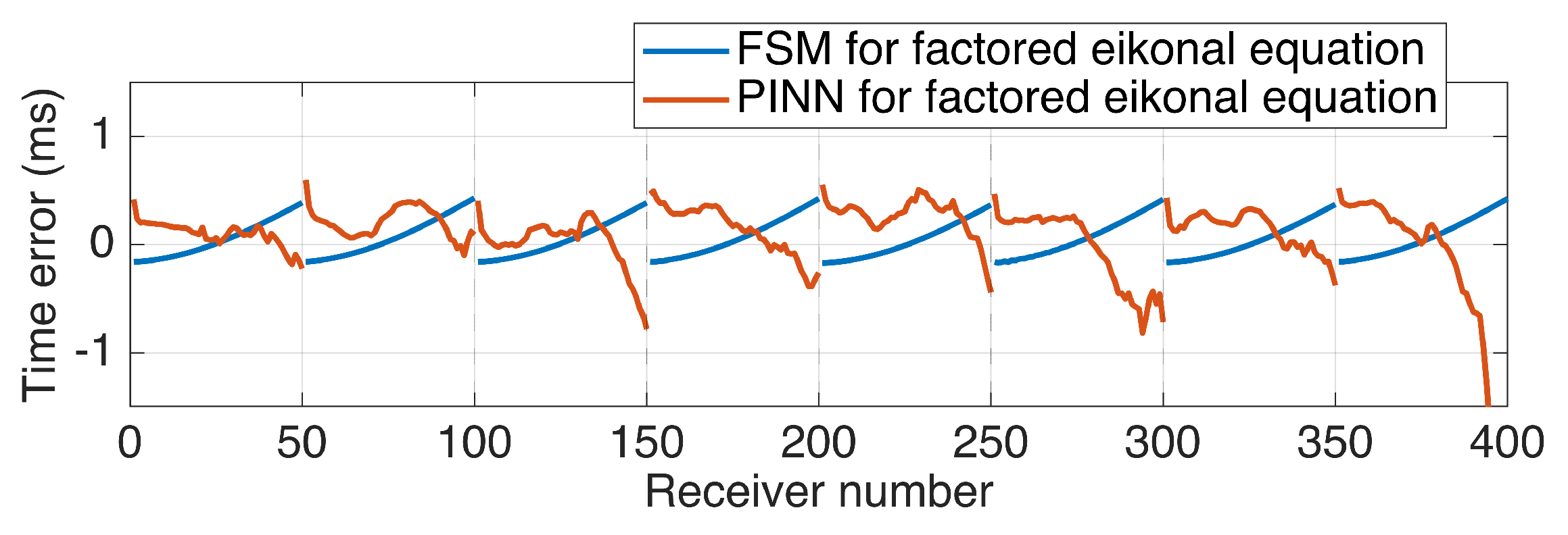
2.3. FSM for the Factored Eikonal Equation

In order to address this issue and obviate the singularity at the source location, Fomel et al. [8] suggested applying the FSM to the factored eikonal equation. The idea is to use an analytical solution $T_0$ of the eikonal equation for a simplified model and then search for correction $\tau$ for this solution. The simplified solution can be the traveltime in a homogeneous model with the same velocity as at the source position or just a distance function between the source and a grid point. A multiplicative factored decomposition suggests that for a model characterized by the slowness

$$S\left(\mathbf{x}\right)=S_0\left(\mathbf{x}\right)\alpha \left(\mathbf{x}\right),$$

(4)

where $S_0\left(\mathbf{x}\right)$ is a reference slowness in the simplified model and $\alpha \left(\mathbf{x}\right)$ is a multiplicative factor. The solution of eikonal equation can be represented as

$$T\left(\mathbf{x}\right)=T_0\left(\mathbf{x}\right)\tau \left(\mathbf{x}\right)$$

(5)

where $T_0\left(\mathbf{x}\right)$ is the solution of eikonal equation in the simplified model $S_0\left(\mathbf{x}\right)$ and:

$$|\nabla T_0{|}^2=S_0^2\left(\mathbf{x}\right),$$

(6)

the $\alpha \left(\mathbf{x}\right)$ is a known scaling factor between the simplified and original model, and $\tau \left(\mathbf{x}\right)$ is the unknown traveltime correction. Substitution of (4) and (5) into (2) yields the factored eikonal equation:

$$T_0^2{|\nabla \tau |}^2+2T_0\tau (\nabla T_0,\nabla \tau )+{\tau }^2{|\nabla T_0|}^2-{\alpha }^2{S}_0^2\left(\mathbf{x}\right)=0.$$

(7)

This equation can be solved at every grid point $\mathbf{C}$ of the model in a similar way as a regular eikonal equation by considering the same eight tetrahedrons, substituting the first order finite difference approximation for $\nabla \tau$:

$$\nabla \tau \approx ({\tau }_C-{\tau }_W,{\tau }_C-{\tau }_S,{\tau }_c-{\tau }_D)·h^{-1},$$

(8)

and applying causality condition:

$${\tau }_C{T}_0\left(\mathbf{C}\right)>{\tau }_S{T}_0\left(\mathbf{S}\right),{\tau }_C{T}_0\left(\mathbf{C}\right)>{\tau }_W{T}_0\left(\mathbf{W}\right),{\tau }_C{T}_0\left(\mathbf{C}\right)>{\tau }_D{T}_0\left(\mathbf{D}\right).$$

(9)

When there are no real roots of the quadratic equation for ${\tau }_C$ or they do not satisfy the causality condition, it is reduced to the 2D case and solved at each face of the tetrahedron separately. If the 2D case does not yield a suitable solution either, the information of $\tau$ is propagated along the edges of the selected triangle using the method of characteristics [8]. For the triangle $\Delta CWD$ the method will yield two solution candidates:

$${\tau }_{WC}=\frac{S\left(\mathbf{C}\right)h+{\tau }_W{T}_0\left(\mathbf{C}\right)}{T_0\left(\mathbf{C}\right)+T_{0x}\delta x},{\tau }_{DC}=\frac{S\left(\mathbf{C}\right)h+{\tau }_D{T}_0\left(\mathbf{C}\right)}{T_0\left(\mathbf{C}\right)+T_{0z}\delta z}.$$

(10)

Here $\delta x$ and $\delta z$ are coordinate shifts from the point C to the points W and D, respectively, i.e., either $+h$ or $-h$ depending on the face of tetrahedron that is currently considered.

In the last step, the solution candidate with a minimal value is selected and used to update $\tau$ at the current grid point. The procedure is repeated for all grid points during the eight sweeps as in the FSM for the regular eikonal equation. The last difference between these two methods is in the initialization procedure: in the case of FSM for a factored eikonal equation a value of “1” instead of zero is assigned to the array of $\tau$ values at the point-source location.

2.4. Eikonal Solution Using Physics-Informed Neural Networks (PINNs)

Conventional numerical algorithms for solving the eikonal equation, such as FSM or FMM, require the same computational effort for perturbations in the source location and/or velocity model. In diffraction stacking-based locations, a dense grid of potential source locations needs to be computed [2] requiring a large number of source calculations, especially in large 3D models. Therefore, we also consider a recently proposed algorithm to solve the eikonal equation using PINNs [9]. Once a randomly initialized neural network is trained to provide traveltimes for a particular source location, additional computations for new source locations can be significantly sped up using this pre-trained network. This technique is referred to as “transfer learning” in the machine learning literature.

To solve the factored eikonal Equation (7), Waheed et al. [9] leverage the capabilities of neural networks as function approximators [11] and define a loss function that minimizes the residual of the underlying factored eikonal equation on a randomly chosen set of training (collocation) points in the computational domain. This is achieved using the following components:

• a deep neural network (DNN) approximation of the unknown traveltime field $\tau (x,y,z)$,
• a differentiation algorithm, i.e., automatic differentiation in this case, to evaluate the partial derivatives of $\tau (x,y,z)$ with respect to the spatial coordinates $(x,y,z)$,
• a loss function incorporating the underlying eikonal equation sampled on a collocation grid, an optimizer to minimize the loss function by updating the neural network parameters.

Let us consider a three-dimensional domain $\mathsf{\Omega }\in {\mathbb{R}}^3$ where $\mathbf{x}=(x,y,z)$ with a point-source ${\mathbf{x}}_s=(x_s,y_s,z_s)$ where $\tau \left({\mathbf{x}}_s\right)=1$. The unknown traveltime factor $\tau$ is approximated by a DNN such that $\tau \left(\mathbf{x}\right)\approx \widehat{\tau }\left(\mathbf{x}\right)=DNN(\mathbf{x};\theta )$, where $\mathbf{x}=(x,y,z)$ are the network’s input, $\widehat{\tau }$ is the network’s output, and $\theta$ represents all trainable parameters of the network. The loss function to train these parameters is given as [9]:

$$\mathcal{I}=\frac{1}{N_I}\sum _{{\mathbf{x}}^{*}\in I}{∥\mathcal{L}∥}^2+\frac{1}{N_I}\sum _{{\mathbf{x}}^{*}\in I}{∥\mathcal{H}(-\widehat{\tau })\left|\widehat{\tau }\right|∥}^2+{∥\widehat{\tau }\left({\mathbf{x}}_s\right)-1∥}^2,$$

(11)

where

$$\mathcal{L}=T_0^2|\nabla \widehat{\tau }{|}^2+2T_0\widehat{\tau }(\nabla T_0,\nabla \widehat{\tau })+{\widehat{\tau }}^2{|\nabla T_0|}^2-{\alpha }^2{S}_0^2\left(\mathbf{x}\right).$$

(12)

The first term in the loss function minimizes the residual of the factored eikonal equation on a set I of $N_I$ training points (${\mathbf{x}}^{*}$), the second term penalizes negative solutions by using the Heaviside function $\mathcal{H}(-\widehat{\tau })$. The final term enforces the boundary condition. Network parameters $\theta$ are then optimized by minimizing this loss function on a set of training points.

Once the DNN is trained, we evaluate the trained neural network on a set of regular grid points in $\mathsf{\Omega }$ to obtain an estimate of the unknown traveltime factor. The final traveltime estimate is obtained by multiplying it with the known traveltime part, i.e.,

$$\widehat{T}\left(\mathbf{x}\right)=T_0\left(\mathbf{x}\right)\widehat{\tau }\left(\mathbf{x}\right).$$

(13)

A workflow detailing the algorithm is shown in Figure 2.

3. Numerical Results

In this section, we compare the performance of regular FSM, factored FSM, and the PINN eikonal solver in microseismic source localization. We begin by highlighting the problem with regular FSM using a homogeneous model and then study the three approaches on a heterogeneous model. The PINN model is implemented using the SciANN package [12]—a high level Tensorflow wrapper for scientific computations. We use a neural network with 9 layers having 20 neurons in each hidden layer and train on 10,000 randomly selected points within the computational domain. Choosing a fraction of the total grid points, allow us to implement the method efficiently as the training cost is directly proportional to the number of training points. Previous studies have found random selection of these points to be the optimal approach [13]. We start with a randomly initialized network for the first source position and then use transfer learning for the following sources, i.e., use the trained network from the previous source as the initial weights for the neural network.

3.1. Homogeneous Model

In the first example, we consider a homogeneous model with P-wave velocity $v_p$ = 4000 m/s and 20 m grid spacing. Here, we test only FSM for the original eikonal equation to demonstrate the issue in the simplest case. We select a symmetrical star-shaped acquisition geometry with each receiver line having 2000 m length and 20 m spacing (Figure 3). The target zone where we search for events with diffraction stacking is located at 2000 m to 2500 m depth range and spans from −1450 m to 1450 m in both horizontal directions. We generate a set of synthetic seismograms corresponding to events (explosive–single polarity) regularly distributed on a horizontal plane at 2200 m depth inside the target zone. We then locate the events with the diffraction stacking method using traveltimes computed with FSM for the original eikonal equation and compare true and diffraction stacking locations using the methodology of Anikiev et al. [1].

The traveltime computation error of FSM times for this model does not exceed 7 ms (relative to the analytical solution). As was mentioned previously, if this error was constant across the monitoring array, it would not affect location accuracy at all and only result in a time shift of the origin time. However, Figure 4 shows that the depth location error reaches 150 m in the center of the acquisition setup and decreases to 20–40 m upon reaching the edge of the tested area for source locations. This error distribution results from the fact that the traveltime error is offset dependent and sources in the center are most affected. Positive values of the depth error mean that events are imaged deeper than their true location. The horizontal error is positive if the estimated event location is closer to the center of the model than the true one. Generally sources are located deeper and closer to the center as a result of the traveltime error.

Comparison of hodographs of the FSM solution with exact traveltimes in the homogeneous model provides an insight into the error behavior (Figure 5). First, we observe that the hodograph curvature of FSM is different from the exact solution, meaning a dependence of the traveltime error on the offset. This curvature is compensated by moving events deeper in the center of the array, resulting in a vertical error. At the same time, the apex of the hyperbola does not change and as a result the horizontal location error remains low except for the boundaries of the target zone where depth error trades off with offset. This observation is consistent with previous publications—the depth of detected microseismic events is the most sensitive parameter for surface monitoring.

Second, the number of receivers with significant moveout change is different for the event in the center of the model (Figure 5a) and for the event close to the edge of the target zone (Figure 5b). This results in larger errors in the center of the model. Note that the hodographs presented in figures are adjusted by a constant time shift in a way that minimizes the rms time error. The absolute traveltime errors are minimal at zero offset (i.e., at the apex of hyperbola).

We do not present results of FSM and PINN for a factored eikonal equation in the homogeneous model, as it converges to the exact solution within the machine precision.

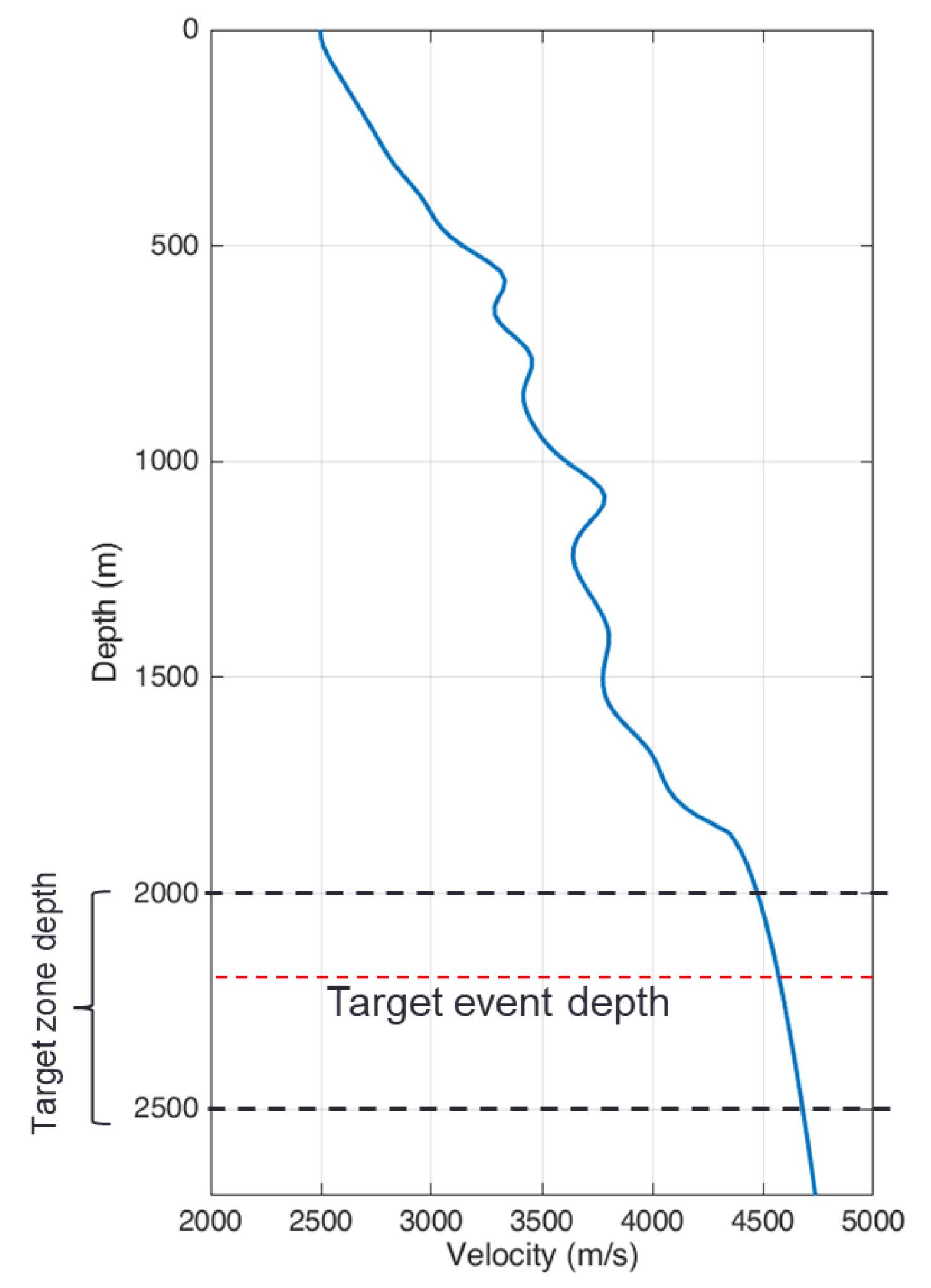
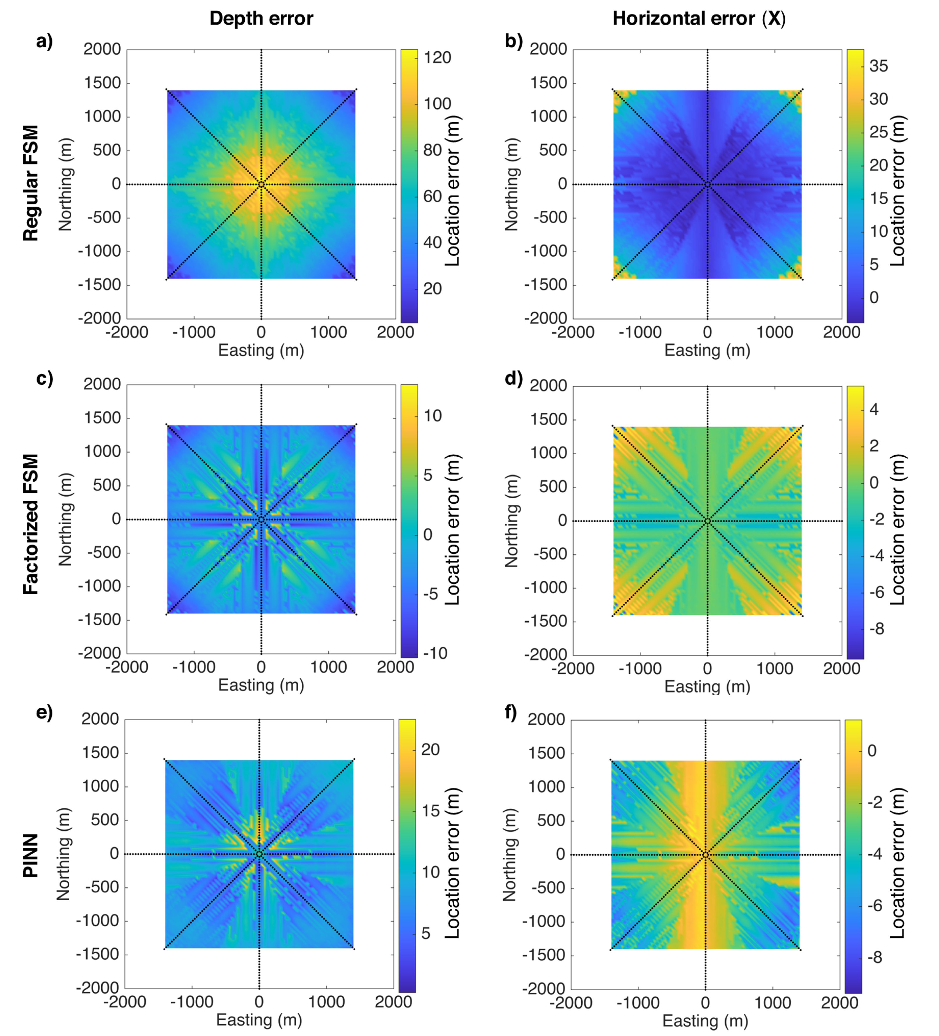
3.2. Heterogeneous Model

In this example, we consider a laterally homogeneous velocity model varying smoothly with depth with a grid step of 20 m (Figure 6). We keep the acquisition setup and target event locations the same as in the above test (homogeneous medium). We again generate a synthetic dataset for a set of events at a fixed depth. Then, we locate these events using the diffraction stacking technique and traveltimes computed from the regular eikonal equation with FSM, the factored eikonal equation with FSM and using the neural network (PINN). Finally, we compare estimated locations with the true locations.

The depth error in case of the regular FSM (Figure 7a) shows a similar pattern as in the homogeneous case: the error is maximal in the center of the acquisition setup and decreases for events closer to the edges of the target zone. The absolute value of the depth error exceeds 120 m, which is significantly larger than the 20 m grid step given the fact that the data is noise free synthetics. In contrast, when traveltimes are computed with the factored FSM, the location error does not exceed half of the grid step for the tested model (Figure 7c). We observe similar location accuracy when utilizing traveltimes computed with PINN. The depth error almost never exceeds the 20 m grid step, though all events now tend to be mislocated deeper into subsurface in contrast to factored FSM, where some of the events have negative depth errors. In addition, the error pictures for PINN are not symmetric any more, since training of the neural network involved stochastic optimization, which introduces random traveltime errors. In case of factored FSM, traveltime errors follow a clear trend and are not random, as shown on the Figure 8.

4. Discussion

We use a rather simple horizontally layered model in order to emphasize how numerical errors from traveltime computation propagate into the location error. If a systematic bias is present in computed traveltimes, it changes the curvature of the hodograph and effectively moves the event location to a different depth. The mislocation distance can be counter-intuitive. If we consider the value of traveltime error, which did not exceed 10 ms for the regular FSM, then a traveltime of 10 ms corresponds to the distance of 40 m, which is how far a P-wave will travel in a medium with average P-wave velocity of 4000 m/s. However, the location error was three times larger and reached 120 m. In the general case, when the velocity model includes lateral heterogeneities, the event’s location will be also shifted in the horizontal direction. Therefore, when choosing an appropriate method for traveltime computation it is important to consider not only the maximal time error but also its variations with offset and propagation direction.

We also note that velocity model is calibrated before locating microseismic events: velocity is adjusted in a way that one or several events with a-priori known locations (check shots, string shots, etc.) are imaged to their correct positions. This calibration will reduce location error associated with inaccurate traveltime computation. However, because there is a strong dependence of the depth error on the horizontal event location, model calibration will improve location accuracy only locally close to the reference event used for calibration.

We have demonstrated that traveltimes, computed with FSM for the regular eikonal equation, introduce significant bias when used for location of microseismic events; they can exceed 100 m for realistic scenarios. The events are shifted deeper and the shift depends on the distance from the center of the acquisition setup. The reason of the bias is a strong dependence of the traveltime error on the propagation direction, which changes the move-out of the arrival times and leads to event mislocations. The FSM for factored eikonal equation effectively addresses this issue by providing significantly more accurate traveltimes. Alternatively, factored eikonal equation can be solved using physics-informed neural networks. Event locations, obtained with this method, have similar accuracy to the factored FSM. However, the location error is more random and less systematically biased. Moreover, PINNs also allow the flexibility of benefiting from transfer learning for updated velocity models, in addition to source positions, as demonstrated by Waheed et al. [9]. Furthermore, since the PINN eikonal solver uses Tensorflow at the backend, it allows easy deployment of computations across a variety of platforms (CPUs, GPUs) and architectures (desktops, clusters). On the contrary, significant effort needs to be spent on adapting the FSM algorithms to benefit from different computational platforms or architectures.

References

1. Anikiev, D.; Valenta, J.; Stanek, F.; Eisner, L. Joint location and source mechanism inversion of microseismic events: Benchmarking on seismicity induced by hydraulic fracturing. Geophys. J. Int. 2014, 198, 249–258. [Google Scholar] [CrossRef] [Green Version]
2. Duncan, P.M.; Eisner, L. Reservoir characterization using surface microseismic monitoring. Geophysics 2010, 75, 75A139–75A146. [Google Scholar] [CrossRef]
3. Chambers, K.; Kendall, J.-M.; Brandsberg-Dahl, S.; Rueda, J. Testing the ability of surface arrays to monitor microseismic activity. Geophys. Prospect. 2010, 58, 821–830. [Google Scholar] [CrossRef]
4. Zhao, H. A fast sweeping method for Eikonal equations. Math. Comput. 2004, 74, 603–628. [Google Scholar] [CrossRef] [Green Version]
5. Sethian, J.A. A fast marching level set method for monotonically advancing fronts. Proc. Natl. Acad. Sci. USA 1996, 93, 1591–1595. [Google Scholar] [CrossRef] [Green Version]
6. Cancela, B.; Ortega, M.; Penedo, M.G. A Wavefront Marching Method for Solving the Eikonal Equation on Cartesian Grids. In Proceedings of the IEEE International Conference on Computer Vision, Santiago, Chile, 7–13 December 2015; pp. 1832–1840. [Google Scholar]
7. Qian, J.; Zhang, Y.T.; Zhao, H.-K. A fast sweeping method for static convex Hamilton-Jacobi equations. J. Sci. Comput. 2007, 31, 237–271. [Google Scholar] [CrossRef]
8. Fomel, S.; Luo, S.; Zhao, H. Fast sweeping method for the factored eikonal equation. J. Comput. Phys. 2009, 228, 6440–6455. [Google Scholar] [CrossRef]
9. Waheed, U.; Haghighat, E.; Alkhalifah, Y.; Song, C.; Hao, Q. Eikonal solution using physics-informed neural networks. arXiv 2020, arXiv:2007.08330. [Google Scholar]
10. Van Trier, J.; Symes, W.W. Upwind finite-difference calculation of traveltimes. Geophysics 1991, 56, 812–821. [Google Scholar] [CrossRef]
11. Hornik, K.; Stinchcombe, M.; White, H. Multilayer feedforward networks are universal approximators. Neural Netw. 1989, 2, 359–366. [Google Scholar] [CrossRef]
12. Haghighat, E.; Juanes, R. SciANN: A Keras wrapper for scientific computations and physics-informed deep learning using artificial neural networks. arXiv 2020, arXiv:2005.08803. [Google Scholar]
13. Raissi, M.; Perdikaris, P.; Karniadakis, G.E. Physics-informed neural networks: A deep learning framework for solving forward and inverse problems involving nonlinear partial differential equations. J. Comput. Phys. 2019, 378, 686–707. [Google Scholar] [CrossRef]
Figure 1. 3D rectangular mesh around the current point C .
Applsci 11 00982 g001
Figure 2. A randomly initialized deep neural network (DNN) is trained on a set randomly selected training points x * with a given slowness model S ( x * ) . The network is minimized with additional inputs at these training points including the known traveltime field T 0 ( x * ) and its spatial derivative T 0 ( x * ) . Once the DNN is trained, it is evaluated on a regular grid ( x ) to yield an estimate of the unknown traveltime τ ^ ( x ) which is then multiplied by T 0 ( x ) providing the estimated traveltime solution T ^ ( x ) .
Applsci 11 00982 g002
Figure 3. Map view (a) and side view (b) of the acquisition setup and target zone used in diffraction stacking.
Applsci 11 00982 g003
Figure 4. Location error in meters for the vertical (a) and horizontal (b) directions after using fast sweeping method (FSM) for the regular eikonal equation in a homogeneous medium.
Applsci 11 00982 g004
Figure 5. Comparison of exact traveltimes and results of FSM in a homogeneous model for event in the center of the model (a) and close to the edge of the target zone (b).
Applsci 11 00982 g005
Figure 6. P-wave velocity model.
Applsci 11 00982 g006
Figure 7. Location error of diffraction stacking in meters using regular FSM (a,b), factored FSM (c,d), and physics-informed neural network (PINN) (e,f) in laterally homogeneous model.
Applsci 11 00982 g007
Figure 8. Comparison of traveltime errors obtained with FSM for the factored eikonal equation and using PINN for an event at the center of the model.
Applsci 11 00982 g008
Publisher’s Note: MDPI stays neutral with regard to jurisdictional claims in published maps and institutional affiliations.