Understanding the Changed Mechanisms of Laser Beam Fusion Cutting by Applying Beam Oscillation, Based on Thermographic Analysis

Abstract

The latest research on applying beam oscillation in laser beam fusion cutting revealed significant process improvements regarding speed and quality. The reason for this increasing process efficiency remains unexplained; however, theoretical investigations suggest the change in energy deposition (respectively heat conduction) as the cause. The present paper aims to analyze the energy deposition by a novel temperature measurement method. For this purpose, a conventional laser beam cutting setup was equipped with beam oscillation technology and a high-speed temperature measurement setup. Various characteristics of the temperature distribution in the process zone (spatial and temporal resolved temperature profiles, maximum and average values, as well as melt pool size) were evaluated for different conditions of beam oscillation (amplitude, frequency, cutting speed). Additionally, the geometrical properties of the process zone, defining the absorptivity have been measured. The comparison with static beam shaping reveals strong temperature volatility, which is induced by the way of energy deposition and an improved absorptivity over a substantial part of the cut front, with the overall result of enhanced heat conduction. For the first time, changed mechanisms applying beam oscillation instead of static beam shaping have been experimentally identified. Based on these measurements, a previously developed explanatory model was not only confirmed but also extended.

1. Introduction

Laser beam fusion cutting (LBFC) is a highly complex process, which has not been completely understood until today. The principle of LBFC is to melt material using a laser beam superimposed by a coaxially high-pressure gas jet that ejects the melt [1,2,3,4]. In general, LBFC is a high-grade established process in industrial fabrication due to its versatility. However, it has still potential for process improvements, especially for thick metal plates, with the result that there is a broad range of research activities that are application oriented as well as fundamentally based.

1.1. Static Beam Shaping to Optimize Laser Beam Fusion Cutting

The application-oriented research focuses on optimizations in the case of LBFC primarily increasing cutting speed or cut edge quality. A cut edge is of high quality by an absence of burr, together with a homogenous smooth surface without striations [5,6,7,8]. Researchers investigated various methods to improve the cutting result, such as controlling the intensity distribution [9,10,11], spot size [7,12,13], spot shape [10,14], and focal position [7,15,16,17,18]. All these methods have in common that they belong to static beam shaping. This means that the properties of the laser beam are modified before the cutting process takes place [19,20]. However, achieving a high cutting speed demands different process conditions than realizing a high quality cut edge [1,2,3,4]. In summary, the achieved process improvements of the static beam shaping methods do not allow a high cutting speed while maintaining high quality for thick metal plates.

1.2. Measurement Methods to Determine the Limiting Mechanisms of Laser Beam Cutting

Fundamental studies investigate the reasons for the compromises in cutting speed and cut edge quality in LBFC. Therefore, correlations between the laser beam, the material, and the gas jet need to be known, which are experimentally difficult to access. Reasons include the complexity of parameter influences, missing analyzing parameters, and methods to characterize the process mechanism and the miniaturized dimensions of the process zone [21,22]. Hence, most knowledge of the process mechanism is based mainly on theoretical considerations. The latest research activities concentrated on developing measurement approaches to obtain detailed insights into the process mechanisms. The energy deposition, respectively heat conduction, was found to be the most important influencing factor for LBFC [1,3,23].

The heat conduction itself is not measurable, but high heat conduction achieves a fast cutting speed as well as a high-quality cut edge and requires a thin melt film with a high temperature difference [1,3,23]. Accessible indicators are the melt film thickness, the melt flow, or the temperature distribution at the cut front. The melt film thickness is addressable by cross-sections of the cut kerf [24,25]. This method is only applicable after finishing the cutting process and requires a high preparation effort. In addition, the melt film thickness during one cut varies depending on the striations. Therefore, a high number of cross-sections per cut have to be performed to gain reliable results. Observing the melt flow is common to draw conclusions about the cutting result [21,22,26,27,28,29,30,31]. Due to the limited accessibility of the process zone, artificial conditions have been created for process observation [21,27,28] or complex experimental setups have been designed [21,22,27,28,29,30], which are not suitable as standard evaluation. Nevertheless, the investigations found that melt flow generates striations [21,27] and influences burr attachment [29]. In addition, the melt flow contains information about the resulting intensity respectively temperature distribution of the process zone [30,32,33]. For this purpose, the angle-dependent absorption of the wavy melt flow has been calculated. These indirect temperature-measuring methods are based on assumptions and simulations. An important result is the strong correlation between the temperature distribution of the process zone and the cut edge quality [26]. Consequently, further measurement setups have been developed to directly address the temperature of the melt film [34,35,36,37,38,39]. The direct temperature measurement differs from the indirect one by a calibration. The process zone to be imaged on the detecting sensor is quite small for laser beam cutting. A sufficient spatial resolution ensures a differentiation of various temperature regions in the process zone. All of the examined direct temperature measurement setups achieve spatial resolution of the complete processing zone just by repositioning of the sensor [34,35,36,37,38,39]. Camera-based measurement setups performed particularly well, as they provide a sufficient temporal resolution in addition [26,38]. The temporal resolution is especially relevant for observing the melt flow or during high-speed cutting. A higher temporal resolution makes the application of the temperature measurement setup more versatile.

1.3. Beam Oscillation to Overcome the Limiting Process Mechanisms

Beam oscillation as a dynamic beam-shaping method is one application-oriented approach to overcome the limitations of static beam shaping and improve LBFC. The principle is based on a superimposed modification of the laser beam movement regarding the feed direction. In contrast to static beam shaping, beam oscillation demonstrates a high potential of process improvements regarding faster cutting speed and advanced cut edge quality at the same time [19,20,24]. Theoretical considerations of fundamental studies suggest the changed spatial energy deposition (respectively, heat conduction) as the reason, which is caused by the alternating laser beam velocity [2,39,40,41]. Previous experimental investigations of the authors [24] presented a reduced heat-affected zone (HAZ) due to beam oscillation. According to the calculations, the reduced HAZ is based not only on a changed spatial energy deposition but also on the temporal distribution [24]. So far, the explanation for why beam oscillation achieves improved cutting results compared to static beam shaping is based exclusively on theoretical considerations.

The present paper aims to experimentally investigate the changed process mechanism of LBFC utilizing beam oscillation instead of static beam shaping. Therefore, the temperature distribution in the process zone has been measured for different beam oscillation conditions (amplitude, frequency, and cutting speed) with static beam shaping as a reference. For this purpose, a novel temperature measurement setup has been designed with a high spatial as well as high frequency temporal resolution and calibration for large temperature ranges. Conclusions on local effects, maximal and average melt pool temperature, and size were drawn from the position- and time-dependent temperature distributions. Moreover, microscopic images using focus stacking to expose the topography of the cut front. This has been correlated with the local absorption in order to assess the amount of laser beam energy deposited. The temperature distribution in combination with all other measured parameters (as cutting speed, cut edge quality, cut front topography, etc.) has been used to validate the theoretical approach of the characteristic energy deposition and enhanced heat conduction. Finally, the previously developed explanatory model [24] has been extended and refined to identify the causes for the process improvements due to beam oscillation.

2. Materials and Methods

2.1. Experimental Setup

2.1.1. Workpiece, Laser Parameters, and Cutting Equipment

Stainless steel plates with 12 mm thickness were used as work pieces. The LBFC experiments were performed with a multimode, continuous-wave fiber laser, operating at a 1.07 µm wavelength. All trials utilized a laser output power of 3 kW and a randomly polarized beam. The beam waist radius was 97 µm with a corresponding Rayleigh length of 2.8 mm. The laser power, beam waist radius, and Rayleigh length were measured by beam diagnostics. Therefore, an optical-based laser measurement device recorded the laser beam geometry in single planes along the optical axis according to DIN EN ISO 11146-2:2015. The laser beam intensity was almost top-hat distributed within the Rayleigh length and otherwise was Gaussian. Nitrogen was applied as an assist gas with 1.8 MPa gas pressure through a conical nozzle with a 3 mm diameter and a 0.7 mm stand-off distance.

Figure 1 represents the experimental setup. Additional components extended the conventional cutting head. Firstly, a highly dynamic scanner (in terms of achievable frequencies) initiated the beam oscillation. Second, a camera measured the temperature distribution in the process zone. The following sections describe both additional components and their functionality in more detail.

2.1.2. Beam Oscillation Due to Highly Dynamic Scanner

A highly dynamic scanner was integrated into the collimated laser beam path. The used scanner achieved oscillation frequencies up to 4 kHz. The maximum obtainable oscillation amplitude depended on the frequency and varied between 0 µm (static beam shaping) and 600 µm.

Longitudinal, linear beam oscillation was used due to the significant process improvements achieved in previous studies [24]. Figure 2 compares the movement of the laser beam for static beam shaping and longitudinal, linear beam oscillation. For static beam shaping as seen in Figure 2a, the relative motion between the laser beam and material is usually generated by moving the cutting head. In case of longitudinal, linear beam oscillation, the feed was superimposed by a periodical forward and backward movement along the cutting direction presented in Figure 2b. In the following, it will only be referred to as beam oscillation.

In the preliminary stages of the current investigation, extensive parameter studies were carried out in order to optimize the process results. Static beam shaping and three different sets of the beam oscillation according to

Table 1. Overview of the analyzed sets of static beam shaping and longitudinal, linear beam oscillation.

Parameter	Set #1	Set #2	Set # 3	Set #4
beam shaping	static	longitudinal, linear
amplitude [µm]	0	300	550	300
frequency [Hz]	0	500	500	2000

were chosen for in-depth analysis. The starting point for the beam oscillation is dataset #2 with 300 µm amplitude and 500 Hz frequency, which obtained the highest improvements in the current investigation. Based on this, on the one hand, the frequency increased to 2000 Hz, and on the other, hand the amplitude increased to 550 µm to represent general tendencies.

2.1.3. High Spatially and Temporally Resolved Temperature Measurement of the Process Zone

The camera unit was coaxially integrated into the beam path with a dichroic mirror, as illustrated in Figure 1. The temperature measurement used the thermal process light emitted by the process zone. An optimal magnification ratio of the relatively small process zone on the camera sensor ensures a high spatial resolution. For this reason, the measurement setup included a magnifying objective. An adjustable focusing of the magnifying objective provided the necessary information about the depth from the cut kerf. The beam path contained a band-pass filter to ensure that the camera detected only the thermal process light. The specifications of the camera unit are summarized in

Table 2. Characteristics of the developed camera-based temperature measurement setup.

Characteristics	Data
wavelength	740 nm ± 10 nm
sensor	CMOS 1/1.2″ (1936 × 1216 px2)
magnification	2:1
dynamic range	73 dB
quantum efficiency	appx. 30% (@740 nm)
sensitivity threshold	7.2 e−
saturation capacity	32,000 e−

.

The measurement setup necessarily required calibration to comply temperature conformity. For this purpose, an LED-based calibration source was used, which was developed at the Fraunhofer IWS [42]. This LED array emitted infrared radiation in a very small spectral band in the wavelength range of 740 nm ± 10 nm, which was directly tuned to the sensitivity range of the camera sensor. The LED array was tested and certified as a calibration standard at the Physikalisch-Technische Bundesanstalt on a black body. For this LED array, the correlation between emitted radiation and corresponding temperature is known. For the developed temperature measuring setup, a known temperature of the LED array was assigned to each measured gray value of the camera signal. In this way, a temperature–gray value–characteristic was determined for the temperature measuring setup, as shown in Figure 3.

According to this procedure, the calibration was valid for the emission coefficient e = 1. The real emission coefficient is decisive to evaluate absolute temperatures. Therefore, Figure 3 contains further calibration curves, where the cut material was assumed as a diffusive gray body with different emission coefficients.

As the emission coefficient depends on the material, the radiation angle (defined by the cut front topography), and the temperature, it is non-uniform within the process zone. This means a complete consideration of the real influence is impossible, and an uncertainty analysis of the temperature measurement is mandatory. When using the emission coefficient e = 1 for evaluation, Figure 4 shows that the measured temperature is always below the real temperature. In addition, the measurement uncertainty grows at an increasing temperature or decreasing emission coefficient.

2.2. Characterization Methods

2.2.1. Cut Edge Quality

There are three main criteria to judge a cut: the cutting speed, the burr, and the surface roughness.

The cutting speed and focal plane were iteratively adjusted to each other in order to determine for each set of Table 1 the lowest burr and surface roughness at the highest possible feed rate. The cutting speed and focal plane were specified to 0.1 m/min and 0.1 mm steps, respectively.

The burr inspection was accomplished as illustrated in Figure 5. A flatbed graphics scanner equipped with matrix CCD sensor technology and an optical resolution of 6400 dpi digitalized the outline of the cut edge. This imaging method does produce distortion-free cut edges. An algorithm divided the cut length of the sample into five sections and detected the maximum burr height in each one. Finally, the measured height values were averaged for evaluation.

Furthermore, average surface roughness R_z measurements were performed according to DIN EN ISO 4288:1998-04 at three different positions: 1 mm below the top surface, in the middle of the plate thickness, and 1 mm above the bottom surface. Details of the evaluation method of surface roughness are depicted in Figure 5. The mean value of the three measurements evaluated the appearance of the cut edge. The stylus tip radius of 2 µm in the measuring plane and the deflection accuracy of 12 nm in the orthogonal plane limited the measuring resolution of the tactile method.

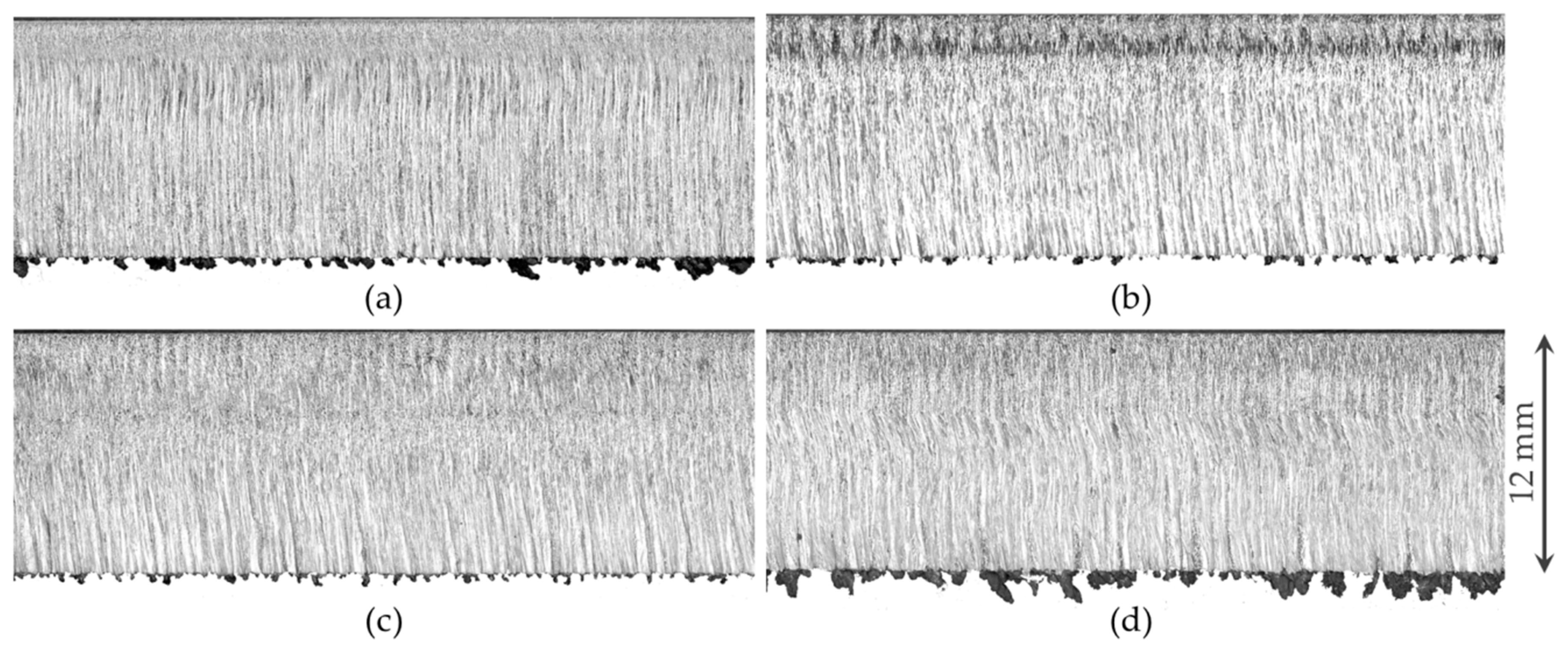
2.2.2. Geometric Properties of Cut Kerf and Cut Front

The validation of the temperature measurement requires knowledge about the position of the cut kerf regarding the camera’s field of view (FOV) as well as the cut front topography. This correlation outlines in Figure 6.

Hence, the cut front was preserved by switching off the laser power during the cutting process but maintaining the feed, so that the gas jet still ejected the melt. Subsequently, the cutting head was repositioned above the point where the laser power switched off (see Figure 6a). A camera image without band pass filter detected the position of the cut kerf within the FOV (see Figure 6b).

A digital microscope, equipped with coaxial illumination and a motorized z-axis, visualized the topography of the cut front. With an optical magnification of 300x (related to a 15 inch monitor), the XY resolution is ≈0.64 µm/px. Hence, focus stacking in 20 µm steps obtained the necessary 3D-depth information of the cut kerf in several layers. This procedure illustrates Figure 6a through the dotted semicircles along the cut front. The cut front topography was used to evaluate the local absorptivity in terms of angle dependence.

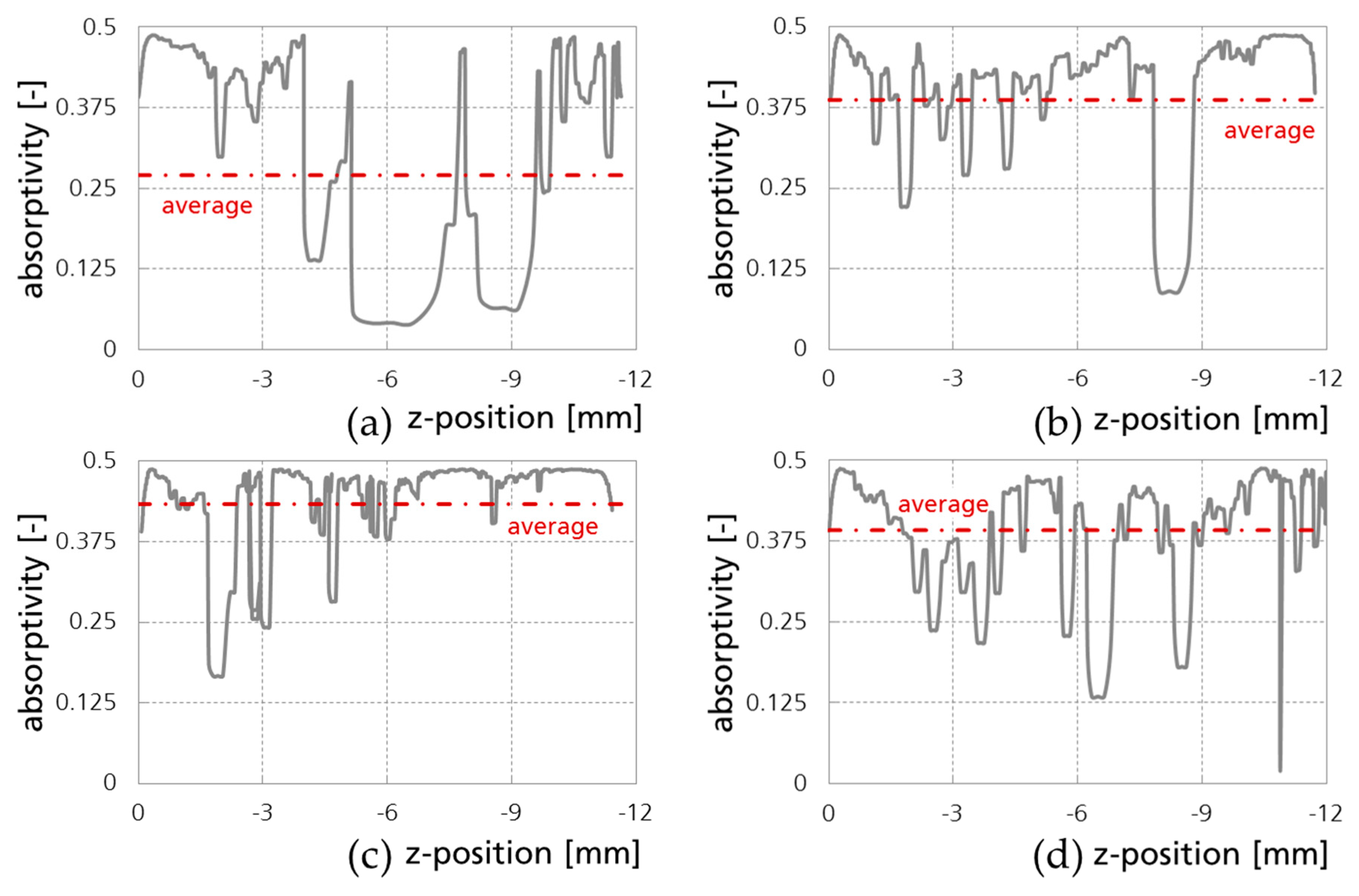
2.2.3. Evaluation of Absorptivity along the Cut Front

The inclined cut front throughout the plate thickness characterizes the transition from solid to molten phase in laser beam cutting. The angle of incidence of the laser radiation on the cut front determines the local absorptivity (see Figure 7), which is associated to the energy deposition and the resulting temperature distribution. According to Figure 6, microscopic imaging using focus stacking recorded a 3D profile of the cut front. Based on these profiles, the local angle of incidence φ_in along the symmetry plane of the cut front was determined (see Figure 7a).

The dependency between the angle of incidence and the reflectivity of polarized laser radiation specifies the Fresnel equations. The present trend of the absorptivity shown in Figure 7b was calculated according to the dissipation of laser energy on metallic surfaces [2]. The absorptivity relates to the polarization state of the laser beam. In case of randomly polarized, respectively non-polarized radiation, it was appropriate to calculate the circularly polarization. The average absorptivity A_Cir for circularly polarized laser radiation defines the relation of reflectivity for parallel and perpendicular radiation R_P and R_S:

$${\mathrm{A}}_{\mathrm{Cir}}=1-\frac{{\mathrm{R}}_{\mathrm{P}}+{\mathrm{R}}_{\mathrm{S}}}{2}.$$

(1)

Whereas the angle dependent reflectivity’s results from the Fresnel equations:

$${\mathrm{R}}_{\mathrm{P}}=\frac{{\left(\mathrm{n}·\cos {\mathsf{\phi }}_{\mathrm{in}}-1\right)}^2+{\left(\mathrm{k}·\cos {\mathsf{\phi }}_{\mathrm{in}}\right)}^2}{{\left(\mathrm{n}·\cos {\mathsf{\phi }}_{\mathrm{in}}+1\right)}^2+{\left(\mathrm{k}·\cos {\mathsf{\phi }}_{\mathrm{in}}\right)}^2},$$

(2)

$${\mathrm{R}}_{\mathrm{S}}=\frac{{\left(\mathrm{n}-\cos {\mathsf{\phi }}_{\mathrm{in}}\right)}^2+{\mathrm{k}}^2}{{\left(\mathrm{n}+\cos {\mathsf{\phi }}_{\mathrm{in}}\right)}^2+{\mathrm{k}}^2},$$

(3)

with the local angle of incidence φ_in, the refractive index n, and the extinction coefficient k. Specific material constants, the wavelength of the laser radiation, and the temperature define the optical parameters n and k. For the present case of laser beam cutting of steel material with a wavelength of λ = 1.07 µm, it was proven to estimate average values for the optical parameters with n = 5.3 and k = 3.82 based on liquid iron [2].

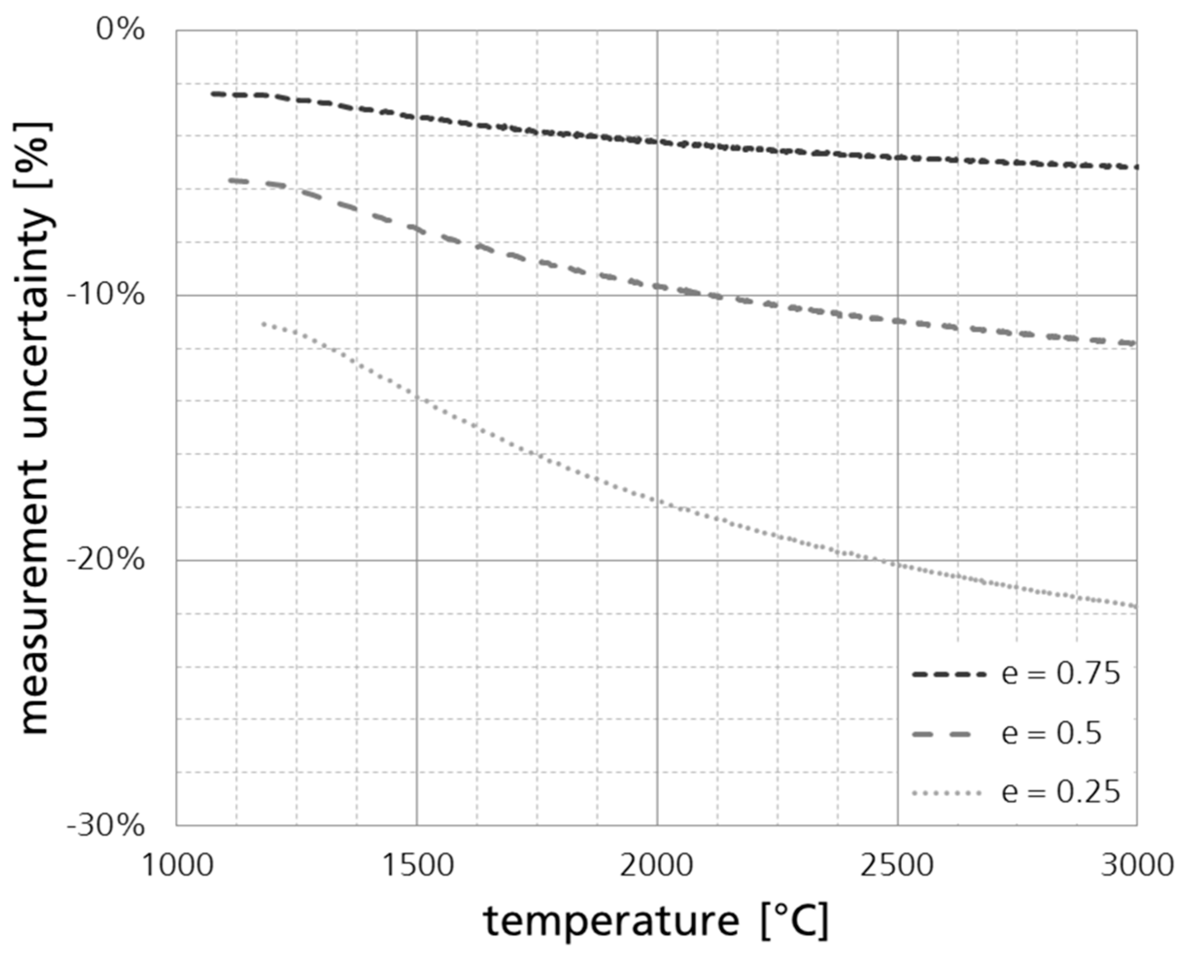
2.2.4. Temperature Distribution

The FOV was adapted to the width of the cut kerf considering a maximum reachable frame rate. Set #1, the static beam shaping, utilized FOV 1 (see Figure 6b). As the cut kerf width decreased for beam oscillation, FOV 2 was applied. As it covered more than half of the process zone, flipping the image at the symmetry axis complemented the missing information. With this method, the frame rate significantly enhanced. The parameters of both FOVs are summarized in

Table 3. Overview of the camera’s FOV in dependence of the analyzed sets.

Parameter	FOV 1	FOV 2
set	#1	#2–#4
m × n [px]	1200 × 300	1200 × 80
image size [mm2]	3.6 × 0.9	3.6 × 0.24
frame rate [FPS]	488	1360

.

The relation between process emission and temperature is shown in Figure 8. The camera recorded gray value images comparable to Figure 8a within the selected FOV. The gray values were converted into the temperature distribution of the process zone using the calibration curve of Figure 3 with the emission coefficient of e = 1. The choice of e = 1 was made deliberately, because the genuine emission coefficient cannot be determined. Additionally, it is not uniform within the process zone. As a consequence, the real temperature will always be higher than the calculated values (within the uncertainty range; see Figure 4). However, working with absolute temperatures allows for more advanced evaluations, such as estimating the melt pool size. The transformed result projected into the cut kerf is shown in Figure 8b.

The camera recorded a sequence of single images over a time period of 500 ms. Each single gray value image was written as matric T_i,j(t). These matrices had the dimensions m × n according to Table 3 and were evaluated in different ways, as described in the following.

Extracting single rows T_i(t) out of the matrices along the cut front (red dashed line in Figure 8b) enabled spatially resolved temperature profiles. These provided e.g., the position of the laser beam regarding the cut front.

Calculating the average ${\overline{\mathrm{T}}}_{\mathrm{i},\mathrm{j}}$ and maximum ${\mathrm{T}}_{\mathrm{i},\mathrm{j}}^{\max }$ temperature matrices out of all single images within a sequence surveyed the characteristic temperature distribution of each set:

$${\overline{\mathrm{T}}}_{\mathrm{i},\mathrm{j}}=\frac{1}{0.5\mathrm{s} · \mathrm{framerate}}{{\displaystyle \sum }}_{0\le \mathrm{t}\le 0.5\mathrm{s}}{\mathrm{T}}_{\mathrm{i},\mathrm{j}}\left(\mathrm{t}\right),$$

(4)

$${\mathrm{T}}_{\mathrm{i},\mathrm{j}}^{\max }=\underset{0\le \mathrm{t}\le 0.5\mathrm{s}}{\max }\left({\mathrm{T}}_{\mathrm{i},\mathrm{j}}\left(\mathrm{t}\right)\right).$$

(5)

To validate the temperature volatility, the mean value of a smaller submatrix $\overline{{\mathrm{T}}_{\mathrm{p},\mathrm{p}}}\left(\mathrm{t}\right)$ out of T_i,j(t) was calculated:

$$\overline{{\mathrm{T}}_{\mathrm{p},\mathrm{p}}}\left(\mathrm{t}\right)=\frac{1}{{\mathrm{p}}^2}{\displaystyle \sum }_{\mathrm{i}=\mathrm{a},\mathrm{j}=\mathrm{b}}^{\mathrm{a}+\mathrm{p},\mathrm{b}+\mathrm{p}}{\mathrm{T}}_{\mathrm{i},\mathrm{j}}\left(\mathrm{t}\right).$$

(6)

The calculations utilized p = 20 pixels, which corresponds to an area of 60 × 60 µm², which are located around the hottest pixel of the cut front. The location is defined by the start coordinates a and b. Plotting $\overline{{\mathrm{T}}_{\mathrm{p},\mathrm{p}}}\left(\mathrm{t}\right)$ versus time visualized a temporally resolved temperature sequence. This sequence revealed the temperature at a fixed position with respect to the moving cut front. To analyze the melting progress, respectively the heating up and cooling periods, a fixed material position was analyzed as well. For that purpose, the temperature $\overline{{\mathrm{T}\prime }_{\mathrm{p}\left(\mathrm{t}\right),\mathrm{p}}}\left(\mathrm{t}\right)$ within the matrix of 20 × 20 pixel with a continuously changing pixel coordinate a’, regarding the certain cutting speed and frame rate was determined:

$$\overline{{\mathrm{T}\prime }_{\mathrm{p}\left(\mathrm{t}\right),\mathrm{p}}}\left(\mathrm{t}\right)=\frac{1}{{\mathrm{p}}^2}{\displaystyle \sum }_{\mathrm{i}=\mathrm{a}\prime ,\mathrm{j}=\mathrm{b}}^{\mathrm{a}\prime =\mathrm{f}\left(\mathrm{t},{\mathrm{v}}_{\mathrm{c}},\mathrm{framerate}\right)+\mathrm{p},\mathrm{b}+\mathrm{p}}{\mathrm{T}}_{\mathrm{i},\mathrm{j}}\left(\mathrm{t}\right).$$

(7)

Furthermore, global histograms estimated an average melt pool size. These histograms represent cumulated areas with equal temperature located at the cut front.

3. Results

3.1. Cutting Speed and Cut Edge Quality

The present investigation analyzes static beam shaping and three different beam oscillations. The cutting speed and focal plane have been optimized regarding the lowest burr and surface roughness at the highest possible feed rate. The resulting parameters are summarized in

Table 4. Overview of the optimized cutting speed and cut edge quality for static beam shaping and longitudinal, linear beam oscillation. Improvements or degradations compared to static beam shaping have been indicated symbolically and in percentiles.

Parameter	Set #1	Set #2		Set # 3		Set #4
beam shaping	static	longitudinal, linear
amplitude [µm]	0	300		550		300
frequency [Hz]	0	500		500		2000
focal plane [mm]	−10.5	−3.2		3.2		–2.8
cutting speed vc [m/min]	0.5	0.85	+70%	0.7	+40%	0.7	+40%
burr height Ø zburr [mm]	1.1	0.65	−41%	0.78	−29%	1.37	+25%
surface roughness Ø Rz [µm]	79	75	−4%	116	+48%	125	+59%

, and Figure 9 depicts the corresponding cut edges.

The results of set #1 (Figure 9a) correspond to the state-of-the-art LBFC with 3 kW laser power. This is the basis for the comparison with beam oscillation. Set #2 (Figure 9b) achieved the highest cutting speed with a 70% increase. Moreover, the burr has the greatest reduction by 41%. Set #2 is the only one to obtain a slightly reduced surface roughness by 4%. The results of set #2 are remarkable, as they cannot be achieved with static beam shaping with this laser power, even by adapting the focal plane. The extended amplitude in set #3 (Figure 9c) still results in a 40% faster cutting speed and 29% less burr height, but the surface roughness increased by 48%. Raising the frequency in set #4 (Figure 9d) achieves a similar cutting speed as set #3. However, the burr height increased by 25% as well as the surface roughness rise by 59%.

3.2. Cut Kerf Properties

Beam oscillation necessarily influences the mechanisms of LBFC to reveal the process improvements recorded in Table 4. To establish the causes, different aspects of the affected process mechanisms have to be considered. Geometrical information of the cut kerf in relation to the temperature measurements is required. Figure 10 exposes the position of the cut front und cut kerf regarding the camera image. The FOV was tailored to the area of interest, resulting in an image section with a total length of 1.8 mm for all sets. The cutting direction is from the right to the left in each image, so that the cut front is positioned on the left and opens into the cut kerf to the right. The geometric dimensions of the cut front as well as the cut kerf vary between the four sets. The cut kerf width depends directly on the laser beam geometry and focal plane (see Table 4). Therefore, the cut kerf width of static beam shaping (Figure 10a) is much wider than for beam oscillation (Figure 10b–d).

The cut front topography is influenced by the laser beam geometry, cutting speed, focal plane, and in case of beam oscillation, also the amplitude. Through focus stacking, the z-profile of the cut front records is shown in Figure 11. The z-dimension stretches along the plate thickness, and the x-dimension reaches into the cut kerf. The cut front changes over time, as the melting process is dynamic. The recorded z-profile only provides an impression at one point in time and is therefore to be understood as an orientation. The z-profile of static beam shaping is unsteady compared to beam oscillation. Static beam shaping achieves the shortest cut front in the x-dimension, and set #3 achieves the longest. The cut front topographies of set #2 and set #4 are almost identical due to identical amplitudes and comparable focal planes. Nevertheless, the cutting results differ drastically.

3.3. Estimated Absorptivity along the Inclined Cut Front

The dissipation of laser energy depends on the angle-dependent absorptivity along the cut front. Whereby the cut front respectively of the angle of incidence is formed by the entire cutting process. This means that the shape and size of the cut front is influenced by the laser beam geometry, the focal plane, and in case of beam oscillation, also the amplitude. The angle of incidence is obtained as an intermediate result out of the cut front topography (see Figure 11), and finally, the distribution of the local absorptivity is calculated (see Figure 12) according to Formula (1). Figure 12 demonstrates a positive impact of dynamic beam oscillation on the angle-dependent absorptivity. It increases nearly up to the theoretical maximum over a wide range of the cut front.

The obtained absorptivity for static beam shaping (set #1) illustrates Figure 12a. The average absorptivity is determined with 0.27 for set #1. Applying beam oscillation, the absorptivity increases for all evaluated conditions. For set #2 and set #4 (Figure 12b,d), 0.39 is calculated as the average absorptivity. The average value actually increases to 0.43 in the case of set #3 (Figure 12c).

3.4. Temperature Distribution within the Process Zone

This section shows the benefit of each parameter and explains why no single, comprehensive parameter can characterize the temperature distribution. The spatially resolved temperature profiles T_i,j(t) and T_i(t) display single measurement moments that result in the global average and maximum temperature distribution (${\overline{\mathrm{T}}}_{\mathrm{i},\mathrm{j}}$ and ${\mathrm{T}}_{\mathrm{i},\mathrm{j}}^{\max }$). In particular, the spatially resolved temperature profiles are useful for the observation of interesting isolated effects and intended primarily for the purposes of traceability and understanding. From the average and maximum temperature matrices, ${\overline{\mathrm{T}}}_{\mathrm{i},\mathrm{j}}$ and ${\mathrm{T}}_{\mathrm{i},\mathrm{j}}^{\max }$, not only is the temperature recognizable but also geometric information about the cut kerf as well as the cut front. Moreover, global effects are apparent, which are decisive for the cutting result. In particular, the average temperature matrix provides information on local heat accumulation. The maximum temperature matrix allows drawing conclusions where exactly the highest temperatures occur at the cut front. The position is not necessarily congruent with the maximum average temperature (${\overline{\mathrm{T}}}_{\mathrm{i}}$ and ${\mathrm{T}}_{\mathrm{i}}^{\max }$). The global histogram allows a quantitative statement about the melt pool size and its temperature distribution. The temperature volatility of a certain position of the cut front $\overline{{\mathrm{T}}_{\mathrm{p},\mathrm{p}}}\left(\mathrm{t}\right)$ is evaluated to determine effects due to beam oscillation, which additionally influences the melt pool dynamics. Eventually, a single parameter is not able to express local as well as global, time-dependent relationships.

3.4.1. Spatial Temperature Profile

After clarifying the geometrical properties of the cut, Figure 13 shows exemplarily sequences of the four following temperature distributions for each set. The temperature peak for static beam shaping (Figure 13a) remains at almost the same position with a medium temperature level. In contrast, the other sequences (Figure 13b–d) depict alternating temperature distributions regarding position and temperature level. This represents the additional beam movement due to beam oscillation.

A closer consideration of the particular temperature measurements delivers the spatially resolved temperature profiles in Figure 14. The position 0 mm is forerunning to the cut front. Starting at 0 mm, the temperature increases from below melting temperature (1450 °C) until reaching the peak and finally decreases below melting temperature again. As indicated in Figure 13a, the four measurements of set #1 create almost coincident charts in Figure 14a. The peak temperature of set #1 differs between 1939 and 2248 °C during the four measurement moments. The position of the peak temperature changes in the range of 0.33 mm ± 0.02 µm. Approximately the position range above melting temperature (approximately 0.1 to 0.8 mm) belongs to the cut front.

The spatially resolved temperature profiles of the beam oscillations behave quite different than static beam shaping. At first, the four measurement moments of one set are not coincident anymore. Second, beam oscillation achieves distinctly higher peak temperatures. Set #2 (Figure 14b) comprises e.g., temperatures between 2205 and 2543 °C and is comparable with Set #3 (Figure 14c), while set #4 (Figure 14d) reaches the highest temperature at 2797 °C. Third, the rise and fall of the temperature curves is either flatter or steeper compared to static beam shaping. Fourth, the position range above melting temperature is significantly enlarged, which will be further discussed in Section 3.4.4.

3.4.2. Global, Average, and Maximum Temperature Distribution

The spatially resolved temperature profiles of beam oscillation are time and position dependent. In order to draw conclusions about the energy deposition, a global view is more appropriate. This provides the average and the maximum temperature matrices over the complete measurement period of 500 ms. These distribution plots are shown in Figure 15 and Figure 16.

The average temperature distributions (Figure 15) reveal an enlarged area of high temperatures for beam oscillation compared to static beam shaping. Additionally, the varying cut kerf width is examined. Static beam shaping (Figure 15a) involves just the smallest portion of the cut front above the melting temperature. In contrast, beam oscillation (Figure 15b–d) heats a large portion of the cut front. A closer consideration of the melt pool size follows later in Section 3.4.4. Although the four sets reached very different peak temperatures in Figure 14, the average temperature has a much lower spread. The square identifies the varying position of the highest average value. Set #1 (Figure 15a) reaches the highest average temperature with 1890 °C, while the highest average temperature of set #2 (Figure 15b) was 2175 °C. Set #3 (Figure 15c) and set #4 (Figure 15d) lay in between these values with 2025 °C and 2115 °C, respectively. Considering only the average temperature ranges, no big differences are observed.

The maximum temperature distributions in Figure 16 confirm again an enlarged area of high temperatures for beam oscillation compared to static beam shaping (Figure 16a). However, it depicts stronger differences between the sets than the average temperature distributions. Especially the reversal points of the oscillation movement are emphasized in case of beam oscillation (Figure 16b–d). The reason is the alternating oscillation direction with a laser beam velocity dropping to zero. This consequently results in a locally longer interaction time and a perceptible higher energy deposition. As a result of this, the maximum temperature for static beam shaping in set #1 (Figure 16a) with 2250 °C is the lowest compared to set #2 (Figure 16b) with 2665 °C and set #3 (Figure 16c) with 2600 °C. Particularly highlighted is set #4 (Figure 16d) with 2910 °C as the highest measured value in this evaluation. It is noticeable that the reversal point directly located at the cut front (left-hand side of the images) is more emphasized than the reversal point further back in the cut kerf (right-hand side of the images).

Figure 14 depicts higher peak temperatures of beam oscillation compared to static beam shaping for single measurement moments. Figure 16 confirms this as a global effect over the entire cut front. The position of the peak temperatures, marked by the square in Figure 15 and Figure 16, are combined in one chart in Figure 17.

The location of the average and maximum peak temperatures for set #1 (Figure 17a) differ slightly with 15 µm. Observing beam oscillation, the position of the highest maximum temperature is not necessarily congruent with the position of the highest average value. In set #2 (Figure 17b), both temperature peaks shifted toward the beginning of the cut front. This results in 95 µm distance of the peak positions for set #2. The two temperature peaks differ in a distance of about 10 µm for set #3 (Figure 17c). A difference in peak locations is especially evident for set #4 (Figure 17d). The considered positions differ by about 235 µm. The highest average temperature significantly shifted to the rear part of the cut front.

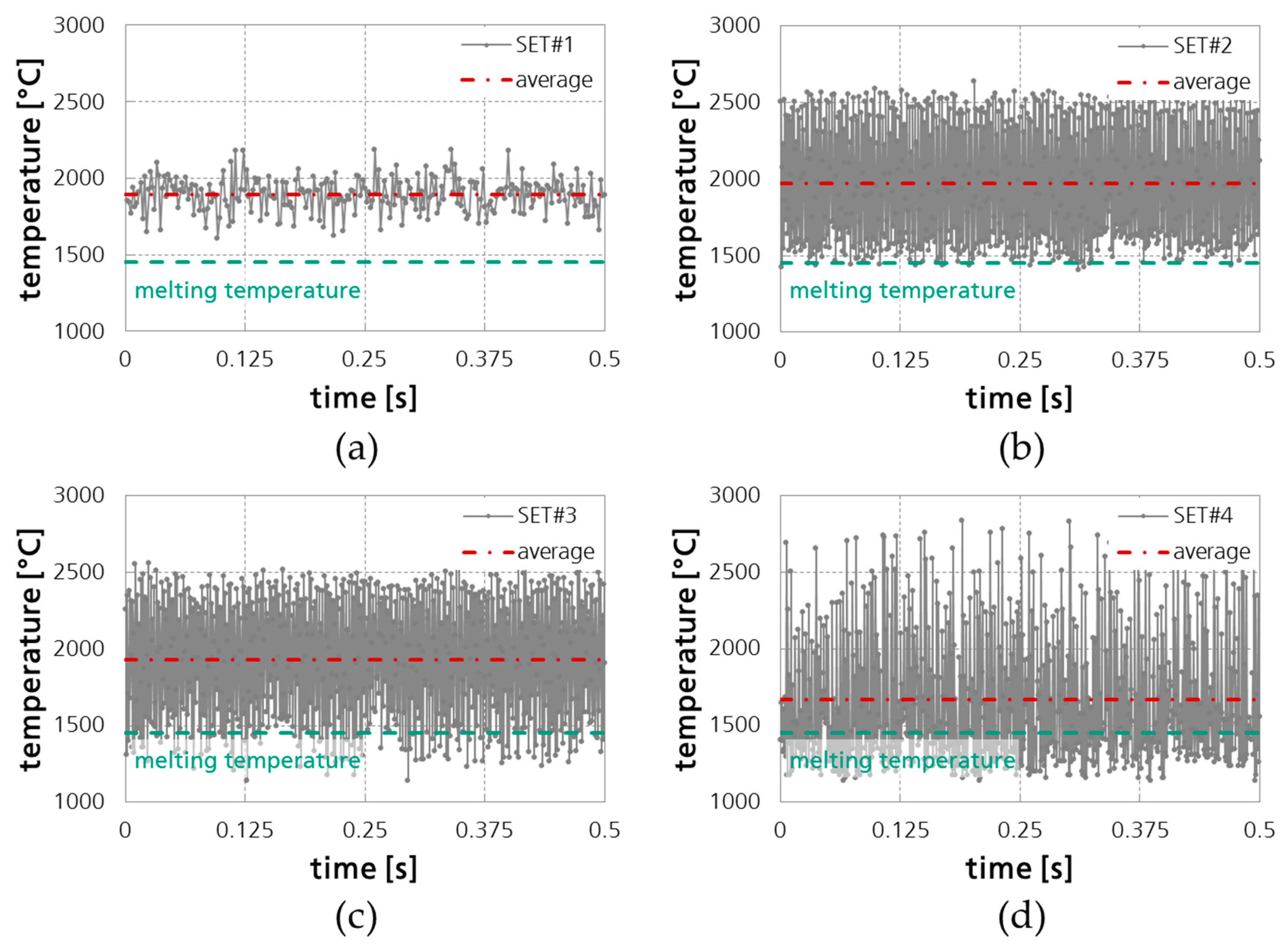
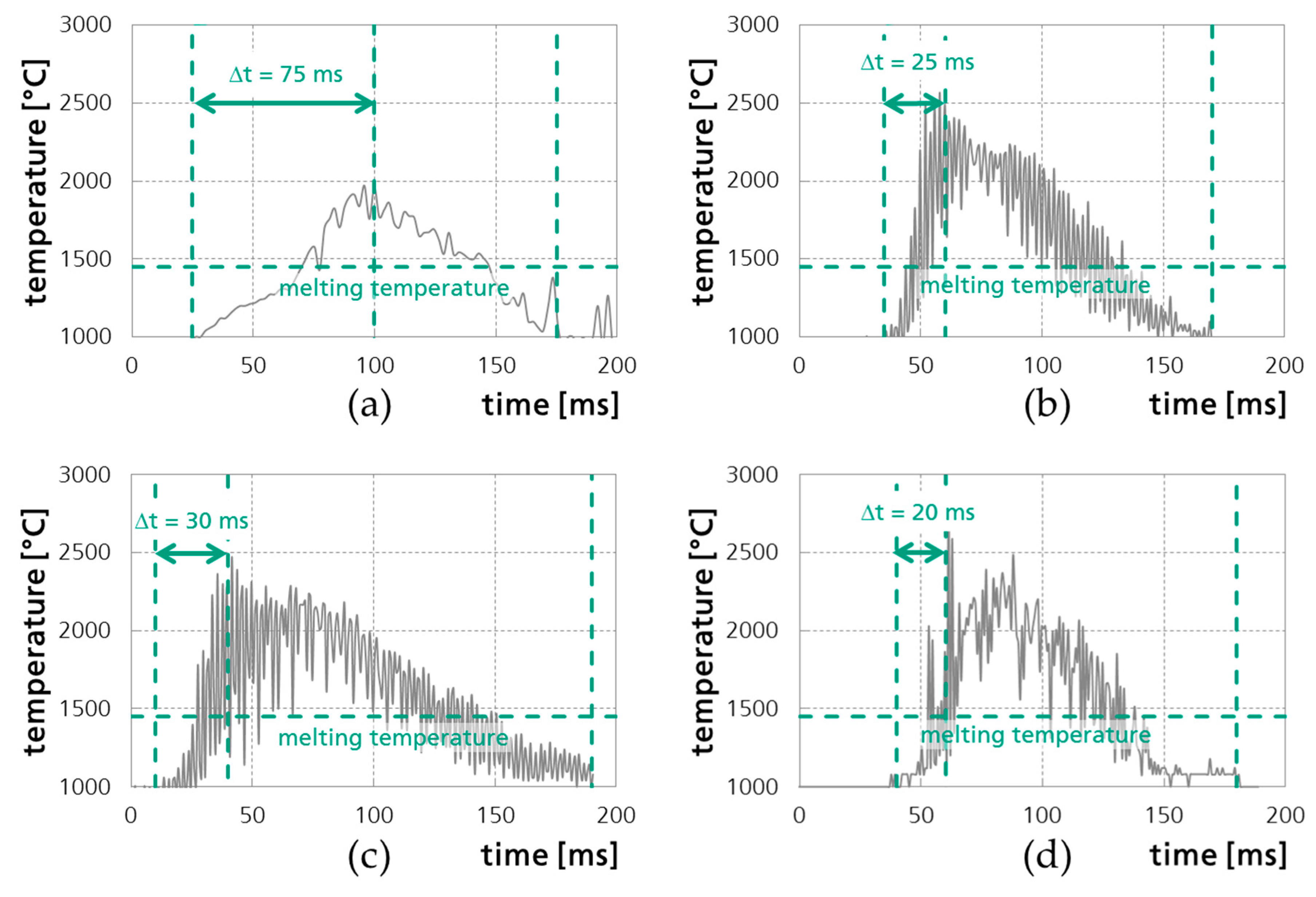
3.4.3. Temporal Temperature Sequence

So far, the spatial and global influence of beam oscillation on the temperature distribution was analyzed. However, the particularity of beam oscillation is its dynamics. For this reason, temporally resolved temperature sequences were created (Figure 18). The origin of the values corresponds to the location of the highest temperatures marked in Figure 16.

The static beam shaping reveals low temperature volatility in Figure 18a. The temperature ranges from 1610 to 2185 °C. So, the temperature difference is calculated with ΔT = 575 °C and an average value of 1890 °C. The temperature volatility significantly increases for beam oscillation (Figure 18b–d). That means that the material position alternately heats up and cools down. The temperatures of set #2 (Figure 18b) decreases to melting temperature and increase up to 2640 °C. The measured temperature difference is ΔT = 1230 °C. Set #3 (Figure 18c) has a slightly higher temperature difference ΔT = 1420 °C but drops partially below the melting temperature. The highest temperature range is in set #4 (Figure 18d), which reaches from below melting temperature up to a 2840 °C peak value. The measured temperature difference is ΔT = 1700 °C.

3.4.4. Melt Pool Size

The last evaluation method of the temperature distribution is the global histogram in order to quantify the melt pool size. Figure 19 confirms the impression of the previous analysis: that the melt pool at the cut front differs significantly for static beam shaping and beam oscillation. The increased hot parts of the melt pool are especially remarkable. The chart shows the cumulated regions of equal temperature, which are averaged for a period of 500 ms. The following example explains the reading method: for static beam shaping (set #1), a temperature of 2000 °C or above is reached within an area of 2000 µm². For beam oscillation, 2000 °C and higher temperatures are measured at an area of 58,000 µm² (set #2), 83,000 µm² (set #3), and 36,000 µm² (set #4). This clearly indicates that high temperatures are only present in a small area of the static beam shaping melt pool. In contrast, beam oscillation exhibits these high temperatures over a larger melt pool area.

In addition, the regions around the melting temperature were considered to acquire the whole melt pool size. This is especially important for static beam shaping, as the temperature distribution illustrates low values at a wide area of the cut front. To identify the borders of the melt pool, an appropriate threshold was defined. Corresponding to Section 2.1.3, the uncertainty analysis is mandatory for this part of the evaluation. Calculating with an emission coefficient of e = 0.25, the melt pool size corresponds very well with the geometric view of Figure 10. Considering Figure 4, this emission coefficient requires a temperature threshold of 1250 °C for the melt pool evaluation. Consequently, as a result, the melt pool size of static beam shaping set #1 is measured out of Figure 19 with 0.65 mm². Applying beam oscillation, the melt pool size is reduced. Set #3 achieves a melt pool size of 0.48 mm², which is a reduction of −26%. Comparable values for the melt pool size are measured for set #2 and set #4, due to the similar amplitude and comparable focal plane. Set #2 achieved 0.37 mm² and set #4 achieved 0.36 mm², which is a reduction of −43% respectively −45% to static beam shaping. Nevertheless, the temperature characteristic and the cutting result differ significant for set #2 and set #4.

4. Discussion

4.1. Estimated Energy Deposition Related to Temperature Evaluation

As stated in the previous publication [24], the energy deposition by applying beam oscillation is no longer uniform but gradual. Analyzing an infinitesimal small part of the workpiece shows this characteristic in Figure 20. For each setup (set #1…#4), the operative part of the laser beam intensity was calculated as a function of time. This was done considering the real laser beam geometry and cutting parameters, according to Table 4. The resulting energy deposition is the cumulative effect of the laser beam intensity. A sufficient energy deposition combined with an adequate interaction time is mandatory to obtain the melting process. Furthermore, a long interaction time is advantageous for an effective melt ejection. The interaction time of the laser beam at a fixed position corresponds to the time starting from the first impact of radiation until the intensity has dropped to zero. This value indicates the maximum interaction time to melt and eject the material. This consideration does not include a real melting process, as well as heat conduction. Therefore, the interaction time is only used as a comparative parameter. For this approach, it suits very well, as it combines the influence of the beam geometry, the beam quality, the focal position, the cutting speed, and the oscillation parameters.

For static beam shaping (Figure 20a), the laser beam intensity steadily increases until the evaluated material position is passed. Subsequently, the intensity decreases in the same manner. During the whole sequence, with an interaction time of about 132 ms, energy is continuously deposited onto the material. Applying beam oscillation, several effects influence the energy deposition. As the focal plane is adapted for set #2, the absolute value of effective intensity clearly increases in Figure 20b. In combination with the increased cutting speed and the oscillating beam, this leads to a shortened interaction time of about 70 ms. The highest intensity is not only valid for one moment, rather, for a long period. This is visible as a kind of intensity plateau in Figure 20b. The increased intensity also leads to a higher amount of deposited energy. The characteristic of energy deposition is obviously gradual due to the pulse-like intensity sequence. Changing the amplitude and focal plane as in set #3 (Figure 20c) results in a slightly decreased cutting speed compared to set #2 (see Table 4). The interaction time significantly increases to 132 ms and is comparable with static beam shaping. However, the intensity and the amount of deposited energy are still at a high level. Applying a high frequency as in set #4 (Figure 20d), the interaction time results in 84 ms due to the decreased cutting speed and the changed focal plane compared to set #2. The denser pulse characteristic and as a result the steadier energy deposition are both remarkable.

It is assumed that the described behavior of gradual energy deposition leads to a distinct volatile temperature profile at the cut front. This was already noticeable within the temperature sequences of $\overline{{\mathrm{T}}_{\mathrm{p},\mathrm{p}}}\left(\mathrm{t}\right)$ in Figure 18. As the position of $\overline{{\mathrm{T}}_{\mathrm{p},\mathrm{p}}}\left(\mathrm{t}\right)$ has a fixed relation to the cut front, only the volatility is evaluable. To consider the interaction time and the heat up phase, a fixed material position with a shifting pixel index needs to be evaluated. This was done with the temporally resolved submatrix $\overline{{\mathrm{T}\prime }_{\mathrm{p}\left(\mathrm{t}\right),\mathrm{p}}}\left(\mathrm{t}\right)$. The result is visualized in Figure 21.

Comparing Figure 20 and Figure 21 reveals similarities, which support the assumption of temperature volatility in dependence of energy deposition. The heat up for static beam shaping (Figure 21a) remains almost uniform until it reaches its maximum of 1975 °C after 75 ms. Set #2 (Figure 21b) reaches the maximum temperature of 2570 °C already after 25 ms. In contrast to static beam shaping, the heat up phase of beam oscillation includes several cooling periods. These cooling periods occur due to the oscillating laser beam, as demonstrated in Figure 20. The decreased laser beam intensity is linked to the moments when the laser beam is not positioned at the cut front. Consequently, the temperature decreases, too (see Figure 21).

The increased maximum temperature is also related to the higher laser beam intensity due to the changed focal position. The fact that a high temperature is reached much faster is based on the oscillation movement. As a result, the peak intensity is immediately applied and, due to its plateau-like characteristics (see Figure 20c,d), it is active for a longer period. Increasing the amplitude as in set #3 (Figure 21c), the heat up to 2470 °C takes around 30 ms. The denser pulses due to the high frequency in set #4 (Figure 21d) enables peak temperatures of 2835 °C even after 20 ms. The interaction times shown in Figure 20 may only qualitatively correspond with the periods shown in Figure 21. Meanwhile, the temperature measurement in Figure 21 represents the real melting process that is also influenced by heat conduction, melt ejection, plate thickness, etc. The estimated energy deposition in Figure 20 does not consider all those circumstances. The important fact is to prove that the interaction time is high for beam oscillation, despite the adjusted focal plane and increased cutting speed. As a general result, the cut front temperature exceeds that of static beam shaping. The following section discusses effects on the cut edge quality.

4.2. Coherence of Temperature Distribution, Energy Deposition, Cut Kerf Properties, and Cutting Result

This chapter analyzes the individual parameters and explains their potential influence on the cutting process. Geometrical as well as thermal and time-dependent parameters and influences have been considered. The aim is to evaluate the changed mechanisms of LBFC by applying beam oscillation.

A first observation is geometrically based: the reduced cut kerf width for beam oscillation (see Figure 10), related to the changed focal plane. In combination with the oscillation amplitude, this defines the melt pool size (see

Table 5. Overview of cutting speed, melt pool size, absorptivity, and interaction time for static beam shaping and longitudinal, linear beam oscillation.

Parameter	Set #1	Set #2	Set # 3	Set #4
beam shaping	static	longitudinal, linear
amplitude [µm]	0	300	550	300
frequency [Hz]	0	500	500	2000
focal plane [mm]	−10.5	−3.2	3.2	−2.8
cutting speed vc [m/min]	0.5	0.85	0.7	0.7
melt pool size [mm2] in Figure 19	0.65	0.37	0.48	0.36
averaged absorptivity [-] in Figure 12	0.27	0.39	0.43	0.39
interaction time [ms] in Figure 20	132	70	132	84

) and therefore the necessary amount of energy to enable a cutting process. The melt pool size decreases for beam oscillation, which allows higher cutting speeds (see Table 5), as less melting energy is needed.

Another geometric influence depends on the cut front topography. The cut front absorbs and converts the laser radiation to thermal energy. The amount of absorbed energy (that enables the melting and cutting process) is limited by the local absorptivity along the cut front. Beam oscillation increases the absorptivity over a wide range of the cut front (see Figure 12 and Table 5). This achieves a continuously flattened cut front. The angle of incidence approaches the theoretical maximum in case of beam oscillation. As a consequence, process efficiency enhances due to the increased energy conversion and reduced transmission losses of laser beam radiation. The cutting speed is additionally increased as a result. With regard to the cutting speed, the interaction time must also be taken into account. The previous section explained how beam oscillation achieves a sufficient interaction time (see Table 5) to ensure a cutting process despite a high cutting speed.

Considering another consequence of the narrow cut kerf width leads to temperature based influences. While for the energy balance, a narrow cut kerf and a small melt pool is favorable, for the melt ejection, it is not [1,3]. With static beam shaping, a focal plane between −3.2 and +3.2 mm is not practical for the evaluated sheet thickness. It would lead to aggravated melt ejection and increased burr formation due to the narrow cut kerf. In combination with a cutting speed higher than 0.7 m/min, this would result in a collapsed cutting process in the worst case. Beam oscillation extends these limitations. Regarding set #1 as reference point, several temperature-based observations have been made. Beam oscillation achieves higher maximum temperatures within the melt pool (see Figure 15, Figure 16, Figure 17, Figure 18, Figure 19 and Figure 20,

Table 6. Overview of burr height, maximum, and average temperatures and temperature volatility for static beam shaping and longitudinal, linear beam oscillation (calculated with e = 1).

Parameter	Set #1	Set #2	Set # 3	Set #4
beam shaping	static	longitudinal, linear
burr height Ø zburr [m/min]	1.1	0.65	0.78	1.37
surface roughness Ø Rz [µm]	79	75	116	125
highest temperature of $T_{i,j}^{max}$ [°C] in Figure 16	2250	2665	2600	2910
average temperature of $\overline{{\mathrm{T}}_{\mathrm{p},\mathrm{p}}}\left(\mathrm{t}\right)$ [°C] in Figure 18	1890	1970	1930	1670
volatility ΔT of $\overline{{\mathrm{T}}_{\mathrm{p},\mathrm{p}}}\left(\mathrm{t}\right)$ °C] in Figure 18	575	1230	1420	1700

). In addition, the average temperature is higher for set #2 and set #3. Overall, this results in low viscosity of the melt film, which improves the melt ejection and supports a reduced burr attachment compared to static beam shaping. Therefore, when applying beam oscillation, it is possible to achieve a good cut edge quality in terms of burr attachment, even in combination with a narrow cut kerf and high cutting speed (e.g., set #2 and set #3).

However, an explanation is still missing as to why not all oscillation parameters, especially set #4, achieve a process improvement. The temperature characteristic within the melt pool has further consequences. Beam oscillation changes the energy deposition compared to static beam shaping. In concrete terms, volatile temperature characteristics with high peak values (see Figure 18b–d and Figure 21b–d) were metrologically verified. Assuming optimal beam oscillation, which is set #2 in this investigation, obtains the following effects: The high peak temperature decreases the viscosity and enhances the temperature difference in the melt film. As stated before, the decreased viscosity improves the melt ejection, which in turn leads to a reduced melt film thickness. As already mentioned, periodic cooling is detectable with the measured temperature volatility. During these cooling periods, the existing melt volume continues to interact with the gas jet. As long as it remains in the molten phase, the cutting gas jet ejects this material. This further reduces the melt film thickness [24]. A high temperature difference within a small melt film thickness attains a high temperature gradient. In turn, the heat conduction rate toward the cutting direction increases. This is an important prerequisite to enhance the cutting speed [1,3,23]. A high temperature gradient is also advantageous for a high-quality cut edge [1,3,23]. These observations are not only valid for set #2, but also set #3. This set has larger amplitude compared to the optimal beam oscillation, which achieves the highest absorptivity (see Table 5). Overall, set #3 results in a good, but slightly lower cut quality compared to set #2 (see Table 4).

In contrast, set #4 does not meet optimal beam oscillation. Although the geometric properties in terms of melt pool size and absorptivity are comparable to set #2, the resulting temperature characteristic, cutting speed, and quality differ significantly. The highest temperatures are only achieved for a small portion of the melt pool (see Figure 19). In concrete terms, only for 800 µm² were the measured temperatures higher than those for set #2. This is equivalent to 0.22% of the melt pool size. Therefore, the largest part of the melt pool remains colder compared to set #2. This mirrors the reduced average temperature in Table 6. Such a low average temperature indicates a high viscosity and results in aggravated melt ejection. Part of the melt remains on the cut edge and leads to an increase in surface roughness. Another part adheres to the bottom side of the sheet and produces the distinct burr attachment. In addition to this explanation, there are additional reasons for the reduced cut edge quality of set #4. A temporally based influence, as the oscillation frequency, is the main difference between set #2 and set #4. It was the highest at set #4 within the investigation. As a consequence, a very high beam velocity is achieved. This results in a low amount of deposited energy per time. The temperature sequence for set #4 is characterized by significant temperature drops (see Figure 18d). It is distinguished by the highest volatility and the lowest average temperature at the cut front for all evaluated sets (see Table 6). The heat conduction losses into the basic material are locally high compared to the amount of deposited energy. In these areas, the temperature drops and the viscosity increases, which in turn leads to aggravated melt ejection. This sustains the inhomogeneous temperature distribution within the melt pool. The position of the highest temperature shifts toward the start of the cut front and is not congruent with the position of the highest average values (see Figure 17d). This indicates very high fluctuation in the viscosity of the melt pool, spatially as well as temporally. Altogether, this destabilizes the melt ejection. As a cutting result, set #4 (Table 4) still enables a feasible cutting speed, but the surface roughness and the burr attachment degraded due to the partly aggravated melt ejection.

A drawback in terms of surface roughness is also obtained for set #3. It represents the experimental setup with the highest amplitude. Compared to set #2, this also results in a higher beam velocity. As visible in Figure 18c, the temperature for the evaluated submatrix $\overline{{\mathrm{T}}_{\mathrm{p},\mathrm{p}}}\left(\mathrm{t}\right)$ drops temporarily below melting temperature compared to set #1 and set #2. In this case, the heat conduction losses temporarily exceed the dissipated laser energy, with the consequence of partial temperature loss. It results in a temporarily higher viscosity and, as stated before, an insufficient melt ejection. In turn, this causes the higher surface roughness.

4.3. Explanatory Model

The present paper aims to explain the changed mechanisms and process improvements due to beam oscillation. The thermographic analysis visualizes the temperature distribution and enables the interpretation of energy deposition and heat conduction. Thus, several aspects characterizing the process zone and the melting process during LBFC have been evaluated. As the main process improvements relate to an increased cutting speed and reduced burr height, this explanation focuses on these properties.

According to the state of the art, an increasing cutting speed requires increased laser beam energy. Static beam shaping realizes this by setting the focal plane near the workpiece surface, enforcing the minimum operative spot size with maximum laser beam intensity. This narrows the cut kerf, causes a small melt volume, and enhances the cutting speed. Simultaneously, the interaction time inevitably decreases, which in turn has a negative effect on the melt ejection. This leads to insufficient melt ejection, degraded cut edge quality, and may provoke a process collapse in the worst case.

By applying beam oscillation, the cumulative energy deposition does not change as long as focal position and cutting speed remain equal to static beam shaping. However, beam oscillation (with sufficient amplitude) extends the interaction time, which influences the melt ejection and cut edge quality. Optimized oscillation and cutting parameters increase the cumulative energy deposition, which enhances the cutting speed. Therefore, by applying beam oscillation, it is feasible to obtain the desired effects in combination: an increasing energy deposition with a simultaneous extended interaction time, which is impossible in the case of static beam shaping. Beam oscillation produces a steady and flat cut front compared to static beam shaping. The changed cut front angle due to beam oscillation enhances the absorptivity over a wide range of the cut front and increases the amount of dissipated energy. Additionally, this increases the peak temperature locally. The named effects are visualized in Figure 22.

The gradual energy deposition causes a volatile temperature distribution, which is characteristic for beam oscillation. The high temperature reduces the viscosity of the melt film, which improves the melt ejection and in turn reduces the burr attachment and surface roughness. The sequential cooling periods of the process zone keep the melt film thin, avoid heat accumulation, and enable efficient melt ejection. A slight melt film thickness in combination with high peak temperatures implies high temperature gradients within the melt film, which accelerates the heat transfer and thus the ongoing melting process. This is another reason for obtaining higher cutting speeds compared to static beam shaping. Thus, the above-described improved melting process in combination with improved melt ejection enables a clearly higher productivity together with high quality. So, all the named aspects—the energy balance, the volatility, the absorptivity and the interaction time—are essential to obtain the named process improvements due to beam oscillation.

References

1. Olsen, F.O. Fundamental mechanisms of cutting front formation in laser cutting. Proc. SPIE 1994, 2207, 402–413. [Google Scholar] [CrossRef]
2. Mahrle, A.; Bartels, F.; Beyer, R.E. Theoretical aspects of the process efficiency in laser beam cutting with fiber lasers. LIA Publ. 2008, 611, 703–712. [Google Scholar] [CrossRef]
3. Wandera, C.; Kujanpää, V. Characterization of the melt removal rate in laser cutting of thick-section stainless steel. J. Laser Appl. 2010, 22, 62–70. [Google Scholar] [CrossRef]
4. Hügel, H.; Graf, T. Laser in der Fertigung. Grundlagen der Strahlquellen, Systeme, Fertigungsverfahren, 3rd ed.; Springer: Berlin, Germany, 2014; pp. 218–259. [Google Scholar]
5. Hilton, P.A. Cutting stainless steel with disc and CO2 lasers. In Proceedings of the 5th LAMP, Kobe, Japan, 29 June–2 July 2009; pp. 1–6. [Google Scholar]
6. Wandera, C.; Salminen, A.; Kujanpää, V. Inert gas cutting of thick-section stainless steel and medium-section aluminum using a high power fiber laser. J. Laser Appl. 2009, 21, 154–161. [Google Scholar] [CrossRef]
7. Wandera, C.; Kujanpää, V. Optimization of parameters for fibre laser cutting of a 10 mm stainless steel plate. Proc. IMechE Part B J. Eng. Manuf. 2011, 225, 641–649. [Google Scholar] [CrossRef]
8. Orishich, A.M.; Malikov, A.G.; Shulyatyev, V.B.; Golyshev, A.A. Experimental comparison of laser cutting of steel with fiber and CO2 lasers on the basis of minimal roughness. Phys. Procedia 2014, 56, 875–884. [Google Scholar] [CrossRef] [Green Version]
9. Laskin, A.; Williams, G.; Demidovich, A. Applying refractive beam shapers in creating spots of uniform intensity and various shapes. Proc. SPIE 2010, 7579, 75790N-1-9. [Google Scholar] [CrossRef]
10. Doan, H.D.; Noaki, I.; Kazuyoshi, F. Laser processing by using fluidic laser beam shaper. Int. J. Heat Mass Transf. 2013, 64, 263–268. [Google Scholar] [CrossRef]
11. Fuse, K. Beam shaping for advanced laser materials processing. Laser Tech. J. 2015, 12, 19–22. [Google Scholar] [CrossRef] [Green Version]
12. Goppold, C.; Zenger, K.; Herwig, P.; Wetzig, A.; Mahrle, A.; Beyer, E.R. Experimental analysis for improvements of process efficiency and cut edge quality of fusion cutting with 1 µm laser radiation. Phys. Procedia 2014, 56, 892–900. [Google Scholar] [CrossRef]
13. Hilton, P.A.; Lloyd, D.; Tyrer, J.R. Use of a diffractive optic for high power laser cutting. J. Laser Appl. 2016, 28, 012014-1-7. [Google Scholar] [CrossRef] [Green Version]
14. Kaakkunen, J.J.J.; Laakso, P.; Kujanpää, V. Adaptive multibeam laser cutting of thin steel sheets with fiber laser using spatial light modulator. J. Laser Appl. 2014, 26, 032008-1-7. [Google Scholar] [CrossRef]
15. Scintilla, L.D.; Tricarico, L.; Wetzig, A.; Beyer, R.E. Investigation on disk and CO2 laser beam fusion cutting differences based on power balance equation. IJMTM 2013, 69, 30–37. [Google Scholar] [CrossRef]
16. Powell, J.; Tan, W.K.; Maclennan, P.; Rudd, D.; Wykes, C.; Engstrom, H. Laser cutting stainless steel with dual focus lenses. J. Laser Appl. 2000, 12, 224–231. [Google Scholar] [CrossRef]
17. Haas, G.J. Adaptive optics. Ind. Laser Solut. 2002, 17, 1–5. [Google Scholar]
18. Laskin, A.; Volp, J.; Laskin, V.; Ostrun, A. Refractive multi-focus optics for material processing. In Proceedings of the 35th ICALEO, San Diego, CA, USA, 16–20 October 2016; LIA: Orlando, FL, USA, 2016; Volume 1402, pp. 1–6. [Google Scholar] [CrossRef]
19. Goppold, C.; Pinder, T.; Herwig, P.; Mahrle, A.; Wetzig, A.; Beyer, E.R. Beam oscillation—Periodic modification of the geometrical beam properties. In Proceedings of the 8th Lasers in Manufacturing Conference, Munich, Germany, 22–25 June 2015; WLT: Munich, Germany, 2015; Volume 112, pp. 1–8. [Google Scholar]
20. Goppold, C.; Pinder, T.; Herwig, P. Transient beam oscillation with a highly dynamic scanner for laser beam fusion cutting. Adv. Opt. Technol. 2016, 5, 61–70. [Google Scholar] [CrossRef]
21. Yudin, P.V.; Kovalev, O.B. Visualization of events inside kerfs during laser cutting of fusible metal. J. Laser Appl. 2009, 21, 39–45. [Google Scholar] [CrossRef]
22. Pocorni, J.; Petring, D.; Powell, J.; Deichsel, E.; Kaplan, A. Measuring the melt flow on the laser cut front. Phys. Procedia 2015, 78, 99–109. [Google Scholar] [CrossRef]
23. Kheloufi, K.; Amara, E.H.; Benzaoui, A. Numerical simulation of transient three-dimensional temperature and kerf formation in laser fusion cutting. J. Heat Transf. 2015, 137, 112101-1-9. [Google Scholar] [CrossRef]
24. Goppold, C.; Pinder, T.; Schulze, S.; Herwig, P.; Lasagni, A.F. Improvement of Laser Beam Fusion Cutting of Mild and Stainless Steel Due to Longitudinal, Linear Beam Oscillation. Appl. Sci. 2020, 10, 3052. [Google Scholar] [CrossRef]
25. Tani, G.; Tomesani, L.; Campana, G.; Fortunato, A. Quality factors assessed by analytical modelling in laser cutting. Thin Solid Films 2004, 453–454, 486–491. [Google Scholar] [CrossRef]
26. Haferkamp, H.; Goede, M.; von Busse, A. Quality monitoring and assurance for laser beam cutting using thermographic process control. Proc. SPIE 1999, 3824, 383–391. [Google Scholar] [CrossRef]
27. Hirano, K.; Fabbro, R. Experimental investigation of hydrodynamics of melt layer during laser cutting of steel. J. Phys. D Appl. Phys. 2011, 44, 105502. [Google Scholar] [CrossRef] [Green Version]
28. Arntz, D.; Petring, D.; Schneider, F.; Poprawe, R. In situ high speed diagnosis—A quantitative analysis of melt flow dynamics inside cutting kerfs during laser fusion cutting with 1 µm wavelength. J. Laser Appl. 2019, 31, 022206-1-10. [Google Scholar] [CrossRef]
29. Stoyanov, S.; Petring, D.; Arntz, D.; Günder, M.; Gillner, A.; Poprawe, R. Investigation on the melt ejection and burr formation during laser fusion cutting of stainless steel. In Proceedings of the 38th ICALEO, Orlando, FL, USA, 7–10 October 2019; LIA: Orlando, FL, USA, 2019; Volume 1402, pp. 1–9. [Google Scholar]
30. Lind, J.; Fetzer, F.; Basquez-Sanchez, D.; Weidensdörfer, J.; Weber, R.; Graf, T. High-speed X-ray imaging of laser cutting process. In Proceedings of the 38th ICALEO, Orlando, FL, USA, 7–10 October 2019; LIA: Orlando, FL, USA, 2019; Volume 303, pp. 1–5. [Google Scholar]
31. Bocksrocker, O.; Berger, P.; Kessler, S.; Hesse, T.; Rominger, V.; Graf, T. Local Vaporization at the Cut Front at High Laser Cutting Speeds. Lasers Manuf. Mater. Process. 2020, 7, 190–206. [Google Scholar] [CrossRef] [Green Version]
32. Amara, E.; Kheloufi, H.; Tamsaout, K.; Fabbro, R.; Hirano, K. Numerical investigations on high-power laser cutting of metals. Appl. Phys. A 2015, 119, 1245–1260. [Google Scholar] [CrossRef]
33. Halm, U.; Niessen, M.; Arntz, D.; Gillner, A.; Schulz, W. Simulation of the temperature profile on the cut edge in laser fusion cutting. In Proceedings of the 10th LiM, Munich, Germany, 24–27 June 2019; WLT: Munich, Germany, 2019; Volume 244, pp. 1–8. [Google Scholar]
34. Grum, J.; Zuljan, D. Analysis of heat effects in laser cutting of steels. J. Mater. Eng. Perform. 1996, 5, 526–537. [Google Scholar] [CrossRef]
35. Dubrov, A.V.; Dubrov, V.D.; Zavalov, Y.N.; Panchenko, V.Y. Application of optical pyrometry for on-line monitoring in laser-cutting technologies. Appl. Phys. B 2010, 105, 537–543. [Google Scholar] [CrossRef]
36. Onuseit, V.; Jarwitz, M.; Weber, R.; Graf, T. Influence of cut front temperature profile on cutting process. In Proceedings of the 30th ICALEO, Orlando, FL, USA, 23–27 October 2011; LIA: Orlando, FL, USA, 2011; Volume 104, pp. 34–39. [Google Scholar]
37. Phi Long, N.; Matsunaga, Y.; Hanari, T.; Yamada, T.; Muramatsu, T. Experimental investigation of transient temperature characteristic in high power fiber laser cutting of a thick steel plate. Opt. Laser Technol. 2016, 84, 134–143. [Google Scholar] [CrossRef]
38. Devesse, W.; De Baere, D.; Guillaume, P. High resolution temperature measurement of liquid stainless steel using hyperspectral imaging. Sensors 2017, 17, 91. [Google Scholar] [CrossRef] [Green Version]
39. Hamie, A.; Ranc, N.; Schneider, M.; Coste, F. Short wavelength pyrometry by photon counting—Application for temperature measurement in laser oxygen cutting. In Proceedings of the 36th ICALEO, Atlanta, GA, USA, 22–26 October 2017; LIA: Orlando, FL, USA, 2017; Volume 606, pp. 1–7. [Google Scholar] [CrossRef]
40. Mahrle, A.; Beyer, R.E. Theoretical aspects of fibre laser cutting. J. Phys. D Appl. Phys. 2009, 42, 175507-1-9. [Google Scholar] [CrossRef]
41. Mahrle, A.; Beyer, R.E. Modeling and simulation of the energy deposition in laser beam welding with oscillatory beam deflection. In Proceedings of the 26th ICALEO, Orlando, FL, USA, 29 October–1 November 2007; Lu, Y., Ed.; LIA: Orlando, FL, USA, 2007; Volume 1805, pp. 1–10. [Google Scholar] [CrossRef]
42. Bonß, S.; Seifert, M.; Hannweber, J.; Karsunke, U.; Kühn, S.; Pögen, D.; Beyer, R.E. Precise contact-free temperature measurement is the formula for reliable laser driven manufacturing processes. In Proceedings of the 9th LANE, Fuerth, Germany, 12–16 September 2016; Volume 1283, pp. 1–9. [Google Scholar]
Figure 1. Schematic design of the experimental setup consisting of a standard cutting head with an integrated highly dynamic scanner to initiate beam oscillation and a camera unit for the high spatial and high frequency temporal resolution temperature measurement.
Applsci 11 00921 g001
Figure 2. Schematic beam movement of (a) Static beam shaping; (b) Longitudinal, linear beam oscillation.
Applsci 11 00921 g002
Figure 3. Temperature–gray value–calibration curves for different emission coefficients.
Applsci 11 00921 g003
Figure 4. Measurement uncertainty as a function of the real temperature and different emission coefficients to correct the measured temperatures.
Applsci 11 00921 g004
Figure 5. Cross-sectional view along the cutting direction verifies the cut edge quality: maximum burr height was detected in five sections, surface roughness Rz was measured along three lines.
Applsci 11 00921 g005
Figure 6. Principle of the camera field of view (FOV): (a) Perspective view of the process zone with cut kerf and front; (b) Top view of the cut front with camera FOVs.
Applsci 11 00921 g006
Figure 7. Derivation of absorptivity based on cut front topography: (a) Scheme of the angle of incidence φin; (b) Dependence between angle of incidence φin and absorptivity ACir for liquid iron and radiation wavelength λ = 1.07 µm [2].
Applsci 11 00921 g007
Figure 8. Correlation between thermographic and geometric information of the process: (a) Gray value of the process light during the cut; (b) Conversion of the gray value into corresponding temperature distribution super positioned with geometry of the cut kerf.
Applsci 11 00921 g008
Figure 9. Cut edges of 12 mm stainless steel cut with the following parameters: (a) Set #1: Static beam shaping; and different values of the longitudinal, linear beam oscillation parameters; (b) Set #2: 300 µm amplitude and 500 Hz frequency; (c) Set #3: 550 µm amplitude and 500 Hz frequency; (d) Set #4: 300 µm amplitude and 2000 Hz frequency.
Applsci 11 00921 g009
Figure 10. Position of the cut front und cut kerf regarding the camera image of 12 mm stainless steel cut with the following parameters: (a) Set #1: Static beam shaping and different values of the longitudinal, linear beam oscillation parameters: (b) Set #2: 300 µm amplitude and 500 Hz frequency; (c) Set #3: 550 µm amplitude and 500 Hz frequency; (d) Set #4: 300 µm amplitude and 2000 Hz frequency.
Applsci 11 00921 g010
Figure 11. Topography of the cut front of 12 mm stainless steel cut with the following parameters: Set #1: Static beam shaping; and different values of the longitudinal, linear beam oscillation parameters; Set #2: 300 µm amplitude and 500 Hz frequency; Set #3: 550 µm amplitude and 500 Hz frequency; Set #4: 300 µm amplitude and 2000 Hz frequency.
Applsci 11 00921 g011
Figure 12. Local absorptivity along the cut front of 12 mm stainless steel cut with the following parameters: (a) Set #1: Static beam shaping; and different values of the longitudinal, linear beam oscillation parameters; (b) Set #2: 300 µm amplitude and 500 Hz frequency; (c) Set #3: 550 µm amplitude and 500 Hz frequency; (d) Set #4: 300 µm amplitude and 2000 Hz frequency.
Applsci 11 00921 g012
Figure 13. Sequence of four measurement moments for temperature distribution Ti,j(t) calculated with e = 1 of 12 mm stainless steel cut with the following parameters: (a) Set #1: Static beam shaping with 488 fps; and different values of the longitudinal, linear beam oscillation parameters with 1360 fps; (b) Set #2: 300 µm amplitude and 500 Hz frequency; (c) Set #3: 550 µm amplitude and 500 Hz frequency; (d) Set #4: 300 µm amplitude and 2000 Hz frequency.
Applsci 11 00921 g013
Figure 14. Spatially resolved temperature profiles Ti(t) calculated with e = 1 along the symmetry axis of the cut front for four measurement moments of 12 mm stainless steel cut with the following parameters: (a) Set #1: Static beam shaping with 488 fps; and different values of the longitudinal, linear beam oscillation parameters with 1360 fps: (b) Set #2: 300 µm amplitude and 500 Hz frequency; (c) Set #3: 550 µm amplitude and 500 Hz frequency; (d) Set #4: 300 µm amplitude and 2000 Hz frequency.
Applsci 11 00921 g014
Figure 15. Distribution of average temperature T ¯ i , j calculated with e = 1 from all single images within the complete measurement period of 500 ms of 12 mm stainless steel cut with the following parameters: (a) Set #1: Static beam shaping; and different values of the longitudinal, linear beam oscillation parameters: (b) Set #2: 300 µm amplitude and 500 Hz frequency; (c) Set #3: 550 µm amplitude and 500 Hz frequency; (d) Set #4: 300 µm amplitude and 2000 Hz frequency; the square marks the submatrix T p , p ¯ ( t ) positioned at the highest average temperature.
Applsci 11 00921 g015
Figure 16. Distribution of maximum temperature T i , j m a x calculated with e = 1 from all single images within the complete measurement period of 500 ms of 12 mm stainless steel cut with the following parameters: (a) Set #1: Static beam shaping; and different values of the longitudinal, linear beam oscillation parameters: (b) Set #2: 300 µm amplitude and 500 Hz frequency; (c) Set #3: 550 µm amplitude and 500 Hz frequency; (d) Set #4: 300 µm amplitude and 2000 Hz frequency; the square marks the submatrix T p , p ¯ ( t ) positioned at the highest maximum temperature.
Applsci 11 00921 g016
Figure 17. Spatially resolved temperature profiles along the symmetry axes of the cut front for average temperature T ¯ i and maximum temperature T i m a x calculated with e = 1 from all single images within the complete measurement period of 500 ms of 12 mm stainless steel cut with the following parameters: (a) Set #1: Static beam shaping; and different values of the longitudinal, linear beam oscillation parameters: (b) Set #2: 300 µm amplitude and 500 Hz frequency; (c) Set #3: 550 µm amplitude and 500 Hz frequency; (d) Set #4: 300 µm amplitude and 2000 Hz frequency.
Applsci 11 00921 g017
Figure 18. Temporally resolved temperature sequences at the position of the submatrix T p , p ¯ ( t ) in Figure 16 of 12 mm stainless steel cut with: (a) Set #1: Static beam shaping; and different values of the longitudinal, linear beam oscillation parameters: (b) Set #2: 300 µm amplitude and 500 Hz frequency; (c) Set #3: 550 µm amplitude and 500 Hz frequency; (d) Set #4: 300 µm amplitude and 2000 Hz frequency.
Applsci 11 00921 g018
Figure 19. Global histogram of the temperature distribution, averaged for a period of 500 ms of 12 mm stainless steel cut with static beam shaping (set #1) and different values of the longitudinal, linear beam oscillation: 300 µm amplitude and 500 Hz frequency (set #2), 550 µm amplitude and 500 Hz frequency (set #3), 300 µm amplitude and 2000 Hz frequency (set #4).
Applsci 11 00921 g019
Figure 20. Comparison of the local intensity profile and energy deposition for one certain material position along the cut path as function of time for the following parameters: (a) Static beam shaping; and different values of the longitudinal, linear beam oscillation parameters: (b) 300 µm amplitude and 500 Hz frequency; (c) 550 µm amplitude and 500 Hz frequency; (d) 300 µm amplitude and 2000 Hz frequency; heat conduction as well as melt ejection have been disregard.
Applsci 11 00921 g020
Figure 21. Comparison of the local temperature for the submatrix T p ( t ) , p ¯ ( t ) calculated with e = 1 showing one certain material position of 12 mm stainless steel along the cut path as function of time for the following: (a) Static beam shaping; and different values of the longitudinal, linear beam oscillation parameters: (b) 300 µm amplitude and 500 Hz frequency; (c) 550 µm amplitude and 500 Hz frequency; (d) 300 µm amplitude and 2000 Hz frequency.
Applsci 11 00921 g021
Figure 22. Abstract representation of the explanatory model.
Applsci 11 00921 g022