A Fast Method for Calculation of Marine Gravity Anomaly

Abstract

Gravity data have been playing an important role in marine exploration and research. However, obtaining gravity data over an extensive marine area is expensive and inefficient. In reality, marine gravity anomalies are usually calculated from satellite altimetry data. Over the years, numerous methods have been presented for achieving this purpose, most of which are time-consuming due to the integral calculation over a global region and the singularity problem. This paper proposes a fast method for the calculation of marine gravity anomalies. The proposed method introduces a novel scheme to solve the singularity problem and implements the parallel technique based on a graphics processing unit (GPU) for fast calculation. The details for the implementation of the proposed method are described, and it is tested using the geoid height undulation from the Earth Gravitational Model 2008 (EGM2008). The accuracy of the presented method is evaluated by comparing it with marine shipboard gravity data. Its efficiency is demonstrated through comparison with the conventional sequential method. The tests demonstrate that the proposed method can be employed for accurately calculating marine gravity anomalies and provides an advantage on computational efficiency.

1. Introduction

With the gradual deepening of global exploration, the ocean, which covers about 70% of the Earth [1], has become a key study area for future resource detection [2]. When studying specific marine areas, large amounts of basic data are usually required due to their wide range. However, collecting gravity data over an extensive marine area is expensive and inefficient. After decades of development, resolving gravity anomalies from the satellite altimetry data has gradually become the mainstream approach for obtaining marine gravity anomalies [3,4,5,6]. For this method, the satellite altimetry data are processed to obtain the sea surface height [3,7,8]. The geoid height undulation can be calculated by subtracting the mean sea height from the obtained sea surface height. Then, the marine gravity anomalies can be inverted from the geoid height undulation. In the literature, the main methods for transforming the geoid height undulation to marine gravity anomalies are: the least squares collocation (LSC) method [9,10], the inverse Stokes formula method (ISF) [11,12], the inverse Hotine formula (IHF) method [13], and the inverse Vening Meinesz formula (IVMF) method [14,15]. The LSC method is a statistical method that involves the calculation of the matrix inversion of corresponding covariance functions and covariance matrices. The sizes of the covariance matrices are related to the numbers of the predicted marine gravity anomalies and the given geoid height undulation. For the calculation of large-scale marine gravity anomalies, the LSC generates large covariance matrices, which leads to the problem of large matrix inversion. Therefore, the LSC method is time-consuming when calculating large-scale marine gravity anomalies. The other three methods all belong to integral equation methods. For the implementation of these methods, both study areas and the integral areas should be divided into many smaller grids. All the divided grids should be involved in the calculation process, which is time-consuming. The singularity problem exists in these three methods. The judgment statements should be used to solve the singularity problem in the calculation, which further increases the computing time.

To accelerate the calculation of marine gravity anomalies, many scholars have employed the fast Fourier transform (FFT) technique into the calculation: Olgiati et al. [16] studied marine gravity anomalies from satellite altimetry using the ISF method in the spectral domain via the FFT technique; Zhang and Blais [13] used the IHF method with the FFT technique to determine marine gravity in the Labrador Sea region; Zhang and Sideris [17] computed marine gravity in the Labrador Sea area using the IHF method with the FFT technique; Andersen and Knudsen [4] applied the FFT technique into the LSC method to determine the global marine gravity field; Hwang [14] implemented the IVMF method using the FFT technique to compute the gravity anomalies over the South China Sea. The FFT technique is sensitive to noise, which would amplify high-frequency errors [4,18]. Therefore, it is necessary to filter the results of the FFT technique. However, the filtering process would remove useful information from the results calculated by the FFT technique. Besides, sometimes, the FFT technique would produce unstable gravity anomalies.

To address the time-consuming geosciences problems, the graphics processing unit (GPU) provides a feasible solution. For example, Chen et al. [19] used GPU parallel computing and the CUDA platform to present a parallel program, GICUDA, a rapid inversion of large-scale gravity and gravity gradiometry data; Zhang et al. [20] introduced a fast forward calculation method of gravity, which was further accelerated using GPU. Based on the platform of GPU, Chen et al. [21] proposed a fast inversion of gravity interface. Liu and Li [22] used a GPU in CUDA to implement prestack Kirchhoff time migration, and so on [23,24].

In this study, we focused on accelerating the calculation of marine gravity anomalies, and we constructed a faster method. In the fast method, we solve the singularity problem in the ISF method without using judgment statements and use GPU parallel computing technology in the implementation of the calculation process. The geoid height undulation data from the EGM2008 (Earth Gravitational Model 2008) model are used to show the accuracy and performance of the proposed fast method.

This paper is organized as follows: In Section 2, the theory of the basic ISF method is described briefly and the details for the fast method are presented. In Section 3, the performance of the proposed fast method is displayed through comparison with the conventional string calculation method. In Section 4, some conclusions and notes are summarized.

2. Method

The free-air gravity anomaly is important in studying specific marine areas. On the ground, the free-air gravity anomaly $\Delta g$ can be obtained by $\Delta g=g_{obs}-g_{fa}-g_0$, where $g_{obs}$ is the observed gravity, $g_{fa}$ is the free-air correction, and $g_0$ is the reference field. Generally, the marine gravity is measured on shipboard. Because the geoid corresponds to sea level, the shipboard gravity minus $g_0$ is the free-air gravity anomaly. The gravity anomaly calculated from the inverse Stokes formula is also the marine free-air gravity anomaly.

2.1. The Inverse Stokes Formula

According to Balmino et al. [11], the inverse Stokes formula, which uses geoid height undulation to calculate marine gravity anomaly, has the form of,

$$\Delta g_p({\phi }_p,{\lambda }_p)=-\frac{\overline{\gamma }}{R}{N}_p-\frac{\overline{\gamma }}{16\pi R}{\displaystyle \underset{\sigma }{\iint }\frac{N_q-N_p}{{\sin }^3\frac{\psi }{2}}}$$

(1)

where ${\phi }_p$ and ${\lambda }_p$ are latitude and longitude coordinates of the point P (the central point of any grid in the study area), respectively; $\Delta g_p$ is the gravity anomaly at point P; $\overline{\gamma }$ is the average gravity of the Earth; $R$ is the average radius of the Earth; $N_p$ is the geoid height undulation at the point P; and $N_q$ is the geoid height undulation at a point Q (the central point of any grid in the integral area) in an integral range. ${\sin }^3\left(\psi /2\right)$ can be computed by:

$${\sin }^3\frac{\psi }{2}={\left({\sin }^2\frac{{\phi }_p-{\phi }_q}{2}+{\sin }^2\frac{{\lambda }_p-{\lambda }_q}{2}\cos {\phi }_p\cos {\phi }_q\right)}^{\raisebox{1ex}{$3$}\!\left/ \!\raisebox{-1ex}{$2$}\right.}$$

(2)

where ${\phi }_q$ and ${\lambda }_q$ are the latitude and longitude coordinates of point Q, respectively. When using Equation (1) to compute the marine gravity anomaly, the integral calculation needs to be carried out in the global region. For ease of calculation, Equation (1) can be converted into a cumulative summation form as:

$$\Delta g_p({\phi }_p,{\lambda }_p)=-\frac{\overline{\gamma }}{R}{N}_P-\frac{\Delta \phi \Delta \lambda }{16\pi R}\overline{\gamma }{\displaystyle \sum _{{\phi }_q={\phi }_1}^{{\phi }_n}{\displaystyle \sum _{{\lambda }_q={\lambda }_1}^{{\lambda }_n}\frac{\left(N_q-N_p\right)\cos {\phi }_q}{{\sin }^3\raisebox{1ex}{$\psi $}\!\left/ \!\raisebox{-1ex}{$2$}\right.}}}$$

(3)

where $\Delta \phi$ and $\Delta \lambda$ are grid intervals along the latitude and longitude directions, respectively; and ${\phi }_n$ and ${\lambda }_n$ are the numbers of the grid along the latitude and longitude directions, respectively.

When point P and point Q coincide, they have the same latitude and longitude coordinates. The term ${\sin }^3(\psi /2)$ in Equation (3) is equal to 0, which leads to a singularity problem. However, the term $N_q-N_p$ in Equation (3) is also equal to 0, and it can be considered that the grid where point Q is located does not contribute to Equation (3). Therefore, when point P and point Q coincide, the corresponding component term $(N_q-N_p)\cos {\phi }_q/{\sin }^3(\psi /2)$ is set to 0, which can solve the singularity problem and does not affect the authenticity of the calculation of Equation (3). Judgment statements are generally used to determine whether point P and point Q coincide. However, the use of judgment statements in a program can increase the computing time. Moreover, the global geoid height undulation data are divided into lots of sufficiently small grids for obtaining a precise marine gravity anomaly. Therefore, the computing time of Equation (3) increases linearly with the number of the grids. To show the characteristics of the gravity anomaly of the study area in detail, the study area is divided into lots of sufficiently small grids to calculate the marine gravity anomalies, which leads to a further increase in the computing time.

2.2. The Proposed Fast Method

In the proposed fast method, the calculation process is improved to avoid judgment statements and GPU parallel computing technology is used to implement the calculation process.

Generally, Equation (3) uses gridded data of global geoid height undulation to compute the marine gravity anomaly of one point. Therefore, a calculation exists of a double loop along the latitude and longitude directions. The marine gravity anomalies of the study area are also computed into gridded data, which leads to another double loop. To reduce the number of loops and simplify the program, the gridded data are transformed into a row vector or a column vector, which is shown in Figure 1, and their latitude and longitude coordinates are transformed into row vectors or column vectors.

The classical method needs to judge whether the calculation point P and the integration point Q coincide. If the two points do not coincide, the integration point Q is incorporated into the calculation of Equation (3). However, the judgment nested within the loop increases the computing time. In the ISF method, the integral area includes the study area, and the integration point Q_p that coincides with calculation point P can be found easily. Therefore, in the proposed fast method, we generate an index vector that records the location (index) of each calculation point P in the integration points (or integral grids). In the calculation of $\Delta g_p({\phi }_p,{\lambda }_p)$, we first calculate each component term $(N_q-N_p)\cos {\phi }_q/{\sin }^3(\psi /2)$ of the cumulative summation part in Equation (3) directly, regardless of the current integration point Q being point Q_p or not. Then, we use the index vector to find the component term $(N_q-N_p)\cos {\phi }_q/{\sin }^3(\psi /2)$ that corresponds to the integration point Q_p and it is set as 0. Finally, we use all of the component terms $(N_q-N_p)\cos {\phi }_q/{\sin }^3(\psi /2)$ to calculate the final value of Equation (3). These operations can solve the singularity problem without judgment statements, which can accelerate the computing process.

Each component term $(N_q-N_p)\cos {\phi }_q/{\sin }^3(\psi /2)$ of the cumulative summation part in Equation (3) can be computed independently, and each marine gravity anomaly in the study area can be computed independently as well. Therefore, GPU parallel computing technology can be used in the proposed fast method.

GPUs were initially used for computer games. Up to now, GPUs have been developed to provide computational power for scientific applications [21]. Parallel computing based on GPUs has been widely applied in geoscience [19,20,21,22,23,24].

MATLAB language has the advantages of powerful data processing capability, easy programming, and numerous multifunctional integrated functions. It can allow the programmer to directly perform GPU computing without knowledge of OpenMP architecture and low-level GPU computing libraries [24]. Therefore, in this study, we used MATLAB language to implement the proposed fast method. The MATLAB code for the proposed fast method is shown in Figure 2. The code in Figure 2 uses the element-wise operation to compute each component term $(N_q-N_p)\cos {\phi }_q/{\sin }^3(\psi /2)$ of the cumulative summation part, which can avoid loops and facilitate parallelization. After setting the component term $(N_q-N_p)\cos {\phi }_q/{\sin }^3(\psi /2)$ corresponding to the integration point Q_p to 0, the sum built-in function of MATLAB is used to compute the cumulative summation part. In the loop, resizing the vector of gravity anomaly each time involves memory deallocation or allocation and value copies, which is time-consuming [25]. Therefore, we preallocated the maximum amount of space required for the vector of gravity anomaly before the loop, and the computing time was reduced further. Given the precision of the results, this code should be performed with double precision.

Here, implementing the fast method includes the following steps:

(1)

Initialize MATLAB.

(2)

Input the gridded data of global geoid height undulation and the corresponding parameters dla (the grid interval along the latitude direction) and dlo (the grid interval along the longitude direction). Transform the gridded data into the vector global_N, and set the corresponding vectors global_la (the latitude coordinate vector of global geoid height undulation) and global_lo (the longitude coordinate vector of global geoid height undulation).

(3)

Input the gridded data of geoid height undulation of the study area. Extract the data in the sea from the gridded data, transform the data in the sea into the vector study_N, and compute the number of elements in the vector study_N (study_number). Set the corresponding vectors study_la (the latitude coordinate vector of geoid height undulation of the study area) and study_lo (the longitude coordinate vector of geoid height undulation of the study area). Compute the index vector pos, which represents the location (index) of the elements of the vector study_N in the vector global_N.

(4)

Set the average_G (the average gravity of the Earth) and R (the average radius of the Earth). Then, use the code as shown in Figure 2 to compute the vector study_Grav (the marine gravity anomaly of the study area).

(5)

Transform the vector study_Grav into gridded data.

(6)

Output the results.

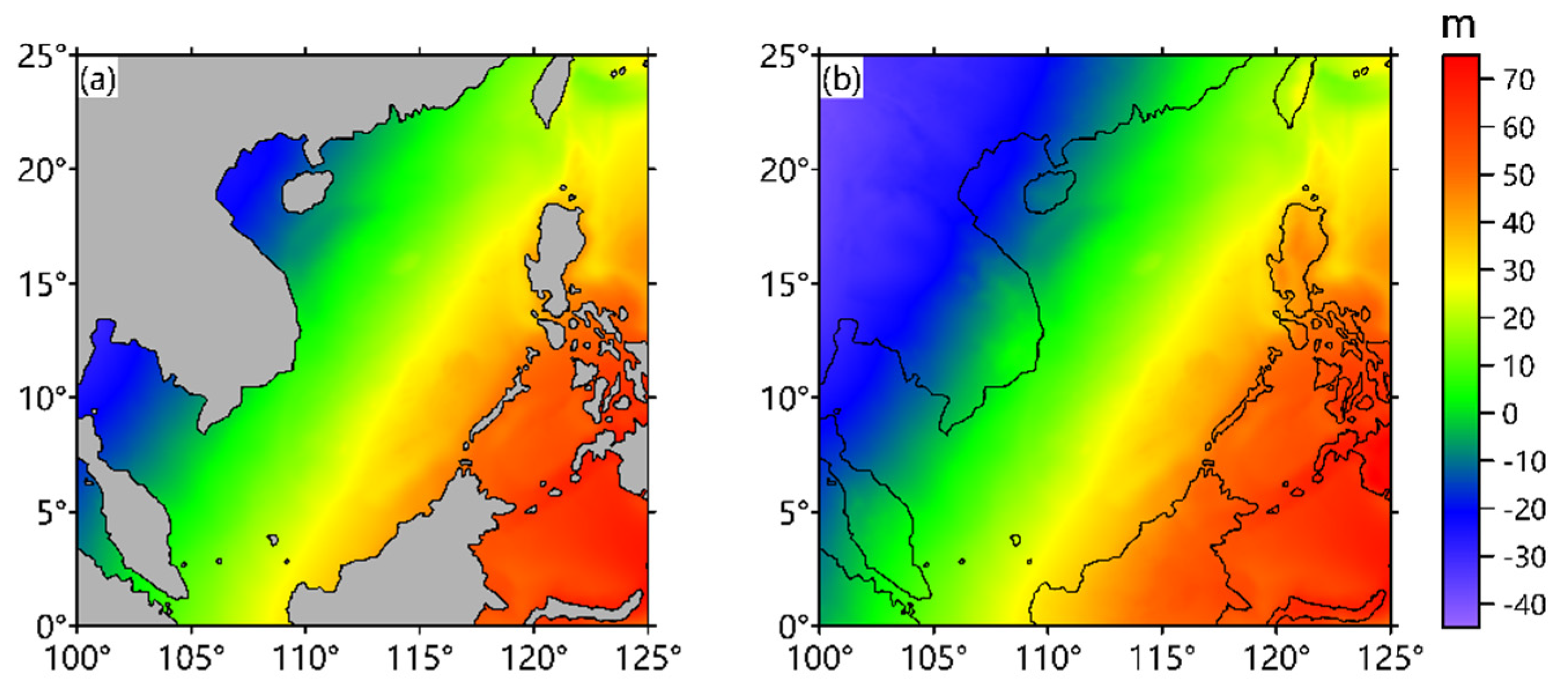
3. Results

We chose the South China Sea as the study area. In the study area, we carried out several tests to show the accuracy and efficiency of the proposed fast method. The geoid height undulation data, which were used in these tests, were all obtained from the EGM2008 model. The geoid height undulation data of the EGM2008 model can be calculated from the file geoidegm2008grid.mat, which can be found on the official website of MATLAB (Appendix A). The following tests were performed on a desktop computer consisting of an Intel^® Core™ i7-9700 CPU 3.00 GHz processor, 32 GB RAM, and an NVIDIA GeForce GTX 1050 Ti GPU card with 4 GB onboard memory. The operating system is Windows 10 64-bit and the platform was MATLAB R2019a.

3.1. Precision and Accuracy Test

Figure 3a shows the geoid height undulation of the South China Sea. The global geoid height undulation is depicted in Figure 4. To obtain accurate marine gravity anomalies with high resolution, we chose the gridded data with 2.5′ × 2.5′ intervals of global geoid height undulation and the geoid height undulation of the South China Sea. The geoid height undulation in the sea was extracted from the gridded data in the South China Sea and used in the calculation. A total of 228,368 points of gravity anomaly needed to be calculated.

The result from the proposed fast method is shown in Figure 5a. The values of the gravity anomalies increase from northwest to southeast as a whole. The gravity anomalies in the middle of the South China Sea extend along the NE or NEE direction, and those in the east and west strike along the NS direction. The gravity anomalies in the local area, whose values vary, show the characteristics of typical marine gravity anomalies, which are associated with continent–ocean transitional zones, spreading ocean ridges, etc.

In GPU parallel computing technology, single-precision produces a result with low precision [26]. Although the result in Figure 5a was calculated in double precision to improve its precision, we still compared it with the result from the classical CPU method to estimate its precision. The result from the classical CPU method is shown in Figure 5b. Figure 5b is similar to Figure 5a, and they have the same trends and characteristics of gravity anomalies. Figure 6 shows the difference between the results in Figure 5a,b. The differences range from −6.47 × 10⁻¹¹ to 7.83 × 10⁻¹¹ mGal, the mean value is −3.77 × 10⁻¹⁵ mGal, and the RMS (root mean square) is 2.78 × 10⁻¹² mGal. Therefore, the precision of the result in Figure 5a is high.

The comparison with the classical CPU method showed that the proposed fast method can calculate the gravity anomalies with high precision, similar to the classical CPU method, but cannot show the accuracy of the result in Figure 5a. A comparison with marine shipboard gravity data can show the accuracy of the result in Figure 5a. Therefore, we collected marine shipboard gravity data. The result in Figure 5a was compared with shipboard gravity data, and Figure 7 shows the spatial distribution of the difference between the result in Figure 5a and the collected marine shipboard gravity data. At the same time, we recorded the statistical parameters of their differences in

Table 1. The difference between the result in Figure 5a and the collected marine shipboard gravity data.

Minimum	Maximum	Mean	Standard Deviation
−15.422 mGal	25.376 mGal	3.990 mGal	9.753 mGal

, which were satisfying and demonstrated that the result in Figure 5a is highly accurate.

3.2. Efficiency Test

We compared the performance of the proposed fast method with the classical method through five tests to demonstrate the efficiency of the proposed fast method. In these tests, for convenience, we used the geoid height undulation of the South China Sea and adjacent land (Figure 3b) to implement tests and did not directly extract the geoid height undulation in the sea. The global geoid height undulation was divided into different grid intervals in each test. The geoid height undulation of the South China Sea and adjacent land was divided into the same grid intervals as the global geoid height undulation in each test. The grid parameters used in each test are displayed in

Table 2. The grid parameters used in each test.

Test No.	Grid Size of the Global Geoid Height Undulation	Grid Intervals of the Global Geoid Height Undulation	Grid Size of Geoid Height Undulation of the Study Area	Grid Intervals of Geoid Height Undulation of the Study Area
1	360 × 180	1° × 1°	25 × 25	1° × 1°
2	720 × 360	0.5° × 0.5°	50 × 50	0.5° × 0.5°
3	1440 × 720	0.25° × 0.25°	100 × 100	0.25° × 0.25°
4	2880 × 1440	0.125° × 0.125°	200 × 200	0.125° × 0.125°
5	5760 × 2880	0.0625° × 0.0625°	400 × 400	0.0625° × 0.0625°

. Three methods were used in every test: (1) the classical method with one CPU core, (2) the classical method with four CPU cores, and (3) the proposed fast method. In each test, each method was executed five times to obtain the corresponding average elapsed time.

Table 3. The elapsed time of the three methods.

Test No.	Classical Method with 1 CPU Core	Classical Method with 4 CPU Cores	Proposed Fast Method	Speedup Ratio 1	Speedup Ratio 2
1	9.237906 s	33.911662 s	1.109683 s	8.324815	30.559774
2	142.453723 s	71.577470 s	7.812566 s	18.233923	9.161839
3	2287.076139 s	666.717880 s	79.818624 s	28.653415	8.352911
4	37913.763020 s	10057.006520 s	1099.028247 s	34.497533	9.150817
5	682715.142000 s	185659.916600 s	16843.824590 s	40.532074	11.022432

Note: Speedup ratio 1 is defined as the ratio of the elapsed time of the classical method with 1 CPU core to the proposed fast method, and speedup ratio 2 is defined as the ratio of the elapsed time of the classical method with 4 CPU cores to the proposed fast method.

shows the elapsed time comparison of these methods. With the increase in the numbers of calculation points and integration points, the elapsed time of every method increases. The proposed method is faster than the other two methods in all tests. Table 3 also shows the speedup ratio of the proposed fast method. Speedup ratio 1 (defined as the ratio of the elapsed time of the classical method with one CPU core to the proposed fast method) increases with the increase in the numbers of calculation points and integration points and eventually reaches 40.532074 in test 5. However, speedup ratio 2 (defined as the ratio of the elapsed time of the classical method with four CPU cores to the proposed fast method) reaches the maximum value in test 1, whose grid size is the smallest in all tests. The reason for this finding is that in test 1, the process of data allocation costs more time than the calculation process. In other tests, the calculation process is the main part, and the time required for the process of data allocation can be neglected. Therefore, speedup ratio 2 decreases in test 2 and 3 and increases in test 4 and 5.

From these tests, we concluded that the proposed fast method could reduce the elapsed time to achieve the purpose of acceleration.

4. Conclusions

We proposed a fast method to accelerate the calculation of marine gravity anomalies. In the fast method, we improved the calculation process of the ISF method and used GPU parallel computing technology. We provided the MATLAB code for the fast method and outlined the steps of this code in detail. We demonstrated the accuracy and efficiency of the proposed fast method for the calculation of large-scale data through several tests.

This proposed fast method is limited by the performance of the GPU cards. If the GPU card has less onboard memory, the proposed method cannot be implemented. Moreover, the accuracy of the result from the proposed method depends largely on the quality and the grid interval of geoid height undulation. The quality of geoid height undulation depends on the qualities of satellite altimetry data and mean sea height, and the grid interval of the geoid height undulation depends on the distribution of satellite orbits. Therefore, before the calculation of the proposed fast method, we should collect satellite altimetry data from numerous satellites with different orbits and the mean sea height with high quality to calculate the geoid height undulation with high quality and a small grid interval.

Both the IHF method and the IVMF method belong to this kind of integral equation method, and they need to overcome the singularity problem. Therefore, after similar corresponding modification, the scheme used in the proposed fast method can also be applied to accelerate the calculation of these two methods.

References

- Li, Y.; Guo, Q.; Huang, M.; Ma, X.; Chen, Z.; Liu, H.; Sun, L. Study of an Electromagnetic Ocean Wave Energy Harvester Driven by an Efficient Swing Body Toward the Self-Powered Ocean Buoy Application. IEEE Access 2019, 7, 129758–129769. [Google Scholar] [CrossRef]
- Li, W.; Chen, G.; Kong, Q.; Wang, Z.; Qian, C. A VR-Ocean system for interactive geospatial analysis and 4D visualization of the marine environment around Antarctica. Comput. Geosci. 2011, 37, 1743–1751. [Google Scholar] [CrossRef]
- Mohanty, K.; Majumdar, T. Altimeter-plot: A C-language program for simultaneous plotting of satellite altimeter-derived geophysical parameters. Comput. Geosci. 1994, 20, 839–848. [Google Scholar] [CrossRef]
- Andersen, O.B.; Knudsen, P. Global marine gravity field from the ERS-1 and Geosat geodetic mission altimetry. J. Geophys. Res. Ocean. 1998, 103, 8129–8137. [Google Scholar] [CrossRef]
- Wan, X.; Ran, J. An alternative method to improve gravity field models by incorporating GOCE gradient data. Earth Sci. Res. J. 2018, 22, 187–193. [Google Scholar] [CrossRef]
- Wan, X.; Ran, J.; Jin, S. Sensitivity analysis of gravity anomalies and vertical gravity gradient data for bathymetry inversion. Mar. Geophys. Res. 2018, 40, 87–96. [Google Scholar] [CrossRef]
- Yang, Y.; Hwang, C.; Hsu, H.-J.; Dongchen, E.; Wang, H. A subwaveform threshold retracked for ERS-1 altimetry: A case study in the Antarctic Ocean. Comput. Geosci. 2012, 41, 88–98. [Google Scholar] [CrossRef]
- Niedzielski, T.; Miziński, B. Automated system for near-real time modelling and prediction of altimeter-derived sea level anomalies. Comput. Geosci. 2013, 58, 29–39. [Google Scholar] [CrossRef]
- Hofmann-Wellenhof, B.; Moritz, H. Physical Geodesy, 2nd ed.; Springer Vienna Publisher: Vienna, Austria, 2006. [Google Scholar]
- Zhu, C.; Guo, J.; Hwang, C.; Gao, J.; Yuan, J.; Liu, X. How HY-2A/GM altimeter performs in marine gravity derivation: Assessment in the South China Sea. Geophys. J. Int. 2019, 219, 1056–1064. [Google Scholar] [CrossRef]
- Balmino, G.; Moynot, B.; Sarrailh, M.; Valès, N. Free air gravity anomalies over the oceans from Seasat and GEOS 3 altimeter data. Eos Trans. Am. Geophys. Union 1987, 68, 17–19. [Google Scholar] [CrossRef]
- Wan, X.; Yu, J. Accuracy analysis of thee remove-restore process in inverse stokes formula. Wuhan Daxue Xuabao 2012, 37, 77–80. (In Chinese) [Google Scholar]
- Zhang, C.; Blais, J.A.R. Comparison of methods for marine gravity determination from satellite altimetry data in the Labrador Sea. Bull. Géodésique 1995, 69, 173–180. [Google Scholar] [CrossRef]
- Hwang, C. Inverse Vening Meinesz formula and deflection-geoid formula: Applications to the predictions of gravity and geoid over the South China Sea. J. Geod. 1998, 72, 304–312. [Google Scholar] [CrossRef]
- Wan, X.; Jin, S.; Liu, B.; Tian, S.; Kong, W.; Annan, R.F. Effects of Interferometric Radar Altimeter Errors on Marine Gravity Field Inversion. Sensors 2020, 20, 2465. [Google Scholar] [CrossRef]
- Olgiati, A.; Balmino, G.; Sarrailh, M.; Green, C.M. Gravity anomalies from satellite altimetry: Comparison between computation via geoid heights and via deflections of the vertical. Bull. Géodésique 1995, 69, 252–260. [Google Scholar] [CrossRef]
- Zhang, C.; Sideris, M.G. Oceanic gravity by analytical inversion of Hotine’s formula. Mar. Geod. 1996, 19, 115–136. [Google Scholar] [CrossRef]
- Andersen, O.B.; Knudsen, P.; Berry, P.A.M. The DNSC08GRA global marine gravity field from double retracked satellite altimetry. J. Geod. 2010, 84, 191–199. [Google Scholar] [CrossRef]
- Chen, Z.; Meng, X.; Guo, L.; Liu, G. GICUDA: A parallel program for 3D correlation imaging of large scale gravity and gravity gradiometry data on graphics processing units with CUDA. Comput. Geosci. 2012, 46, 119–128. [Google Scholar] [CrossRef]
- Zhang, S.; Meng, X.; Chen, Z.; Zhou, J. Rapid calculation of gravity anomalies based on residual node densities and its GPU implementation. Comput. Geosci. 2015, 83, 139–145. [Google Scholar]
- Chen, Z.; Meng, X.; Zhang, S. 3D gravity interface inversion constrained by a few points and its GPU acceleration. Comput. Geosci. 2015, 84, 20–28. [Google Scholar] [CrossRef]
- Liu, G.; Li, C. Practical Implementation of Prestack Kirchhoff Time Migration on a General Purpose Graphics Processing Unit. Acta Geophys. 2016, 64, 1051–1063. [Google Scholar] [CrossRef][Green Version]
- Wang, J.; Meng, X.; Li, F. A computationally efficient scheme for the inversion of large scale potential field data: Application to synthetic and real data. Comput. Geosci. 2015, 85, 102–111. [Google Scholar] [CrossRef]
- Chen, T.; Zhang, G. Forward modeling of gravity anomalies based on cell mergence and parallel computing. Comput. Geosci. 2018, 120, 1–9. [Google Scholar] [CrossRef]
- Suh, J.W.; Kim, Y. Accelerating MATLAB with GPU Computing: A Primer with Examples; Morgan Kaufmann Publisher Inc.: Burlington, MA, USA, 2014. [Google Scholar]
- Moorkamp, M.; Jegen, M.; Roberts, A.; Hobbs, R. Massively parallel forward modeling of scalar and tensor gravimetry data. Comput. Geosci. 2010, 36, 680–686. [Google Scholar] [CrossRef]