Article

Viewport Rendering Algorithm with a Curved Surface for a Wide FOV in 360° Images

Department of Electrical Engineering, Sejong University, Seoul 05006, Korea
*
Author to whom correspondence should be addressed.
Appl. Sci. 2021, 11(3), 1133; https://doi.org/10.3390/app11031133
Submission received: 23 December 2020 / Revised: 21 January 2021 / Accepted: 22 January 2021 / Published: 26 January 2021
(This article belongs to the Section Electrical, Electronics and Communications Engineering)

Abstract

:
Omnidirectional visual content has attracted the attention of customers in a variety of applications because it provides viewers with a realistic experience. Among the techniques that are used to construct omnidirectional media, a viewport rendering technique is one of the most important modules. That is because users can perceptually evaluate the quality of the omnidirectional service based on the quality of the viewport picture. To increase the perceptual quality of an omnidirectional service, we propose an efficient algorithm to render the viewport. In this study, we analyzed the distortions in the viewport picture to be the result of sampling. This is because the image data for the unit sphere in the omnidirectional visual system are non-uniformly sampled to provide the viewport picture in the conventional algorithms. We propose an advanced algorithm to construct the viewport picture, in which the viewport plane is constructed using a curved surface, whereas conventional methods use flat square surfaces. The curved surface makes the sampling interval more equally spaced than conventional techniques. The simulation results show that the proposed technique outperforms the conventional algorithms with respect to the objective quality based on the criteria of straightness, conformality, and subjective perceptual quality.

1. Introduction

Omnidirectional visual content has attracted more attention in the fields of gaming devices, remote lecturing systems, broadcasting, movies, and streaming services because it provides users with a more realistic experience than conventional techniques [1,2,3,4]. Many companies have developed a variety of devices that are related to omnidirectional visual technology. To meet the demands of the industry, the Joint Video Exploration Team (JVET) of ITU-T VCEG (Q6/16) and ISO/IEC MPEG (JTC 1/SC 29/WG 11) has been working on 360° video coding as part of the explorations that are being conducted for developing coding technologies for future video coding standards since 2015 [5,6,7].
An omnidirectional visual system consists of a variety of core technologies, including those for picture capturing, stitching [8,9,10,11], bundle adjustment [12,13], blending [14,15], 360° image formatting [16,17], 360° image encoding [18,19], streaming 360° data [20], and viewport rendering [7]. Recently, stereo omnidirectional visual systems have been introduced to increase the sense of immersion for users. The stereo omnidirectional visual content gives viewers more realistic images and videos [21,22]. Among these essential techniques, viewport rendering is one of the most important modules. Viewport rendering provides users with the final image frames and the users can evaluate the perceptual quality of the omnidirectional visual system based on the quality of the viewport picture (VP) [20,23,24].
During the last decade, many experts have discussed the distortions that have resulted from the various methods to render the VP. Some algorithms bend the straight lines into curved lines in the VP, whereas other methods differently stretch objects in the vertical and horizontal directions. This is because these methods cannot overcome the limitations that result from the geometrical properties of the 360° VR coordinate system.
To solve these problems, many researchers have developed advanced algorithms [25,26,27,28,29,30,31,32]. In a study by Sharpless et al. [25], they modified the cylindrical projection [26] to maintain the shape of the straight lines. An automatic content-aware projection method was proposed by Kim et al. [27]. Kim et al. developed a saliency map to classify the objects in the image according to their importance levels and they combined multiple images to minimize the distortion. In [28], Kopf et al. introduced the locally-adapted projections, where a simple and intuitive user interface allowed the specification of regions of interest to be mapped to the near-planar parts, thereby reducing the bending artifacts. In [29], Tehrani et al. presented the unified solution to correct the distortion in one or more non-occluded foreground objects by applying object-specific segmentation and affine transformation of the segmented camera image plane, where the algorithm was assisted by a simple and intuitive user interface. The algorithm proposed by Jabar et al. [30] moved the center of the projection to minimize the stretching error and bending degradation. Because the algorithms proposed in [27,30] created a saliency map [31] to determine the content of the 360° image, the additional process increased the complexities of these methods. Kopf et al. [32] defined the projected surface of the viewport as the surface of the cylinder, where the size of the cylinder is modified according to the field of view (FOV).
In this study, we consider the distortions in the VP to be the result of sampling because the image data on the unit sphere in the omnidirectional visual system are non-uniformly sampled to provide the VP for conventional algorithms. We propose an advanced algorithm to render the VP, where the viewport plane is constructed using a curved surface, whereas the conventional methods have used flat square surfaces. The curved surface makes the sampling interval more equally spaced than the conventional techniques.
This study is organized as follows. In Section 2, we explain the basic procedure to render the VP and two conventional algorithms: perspective projection [33] and stereographic projection [33]. Some processes are modeled, and we derive some equations to calculate the core parameters. In Section 3, we discuss the limitations of the conventional algorithms and the reasons why the pixels in the VP are distorted. We propose an advanced technique to render the VP in Section 4, where a curved surface is used for the projection plane. In Section 5, we demonstrate the performance of the proposed algorithm and compare it with the various conventional techniques. Finally, the conclusion is presented in Section 6.

2. Conventional Methods to Render the Viewport

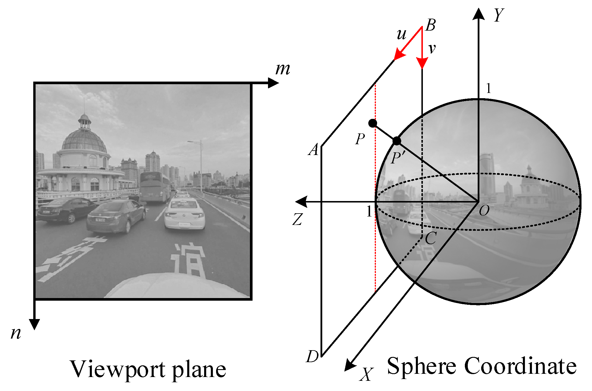
2.1. Basic Procedure to Render the Viewport Picture

Figure 1 shows the 3D XYZ coordinate system that is used to represent the 3D geometry of a 360° image, where the ( X , Y , Z ) coordinates are based on a right-hand coordinate system [7].
The sphere can be sampled with the longitude ( ϕ ) and latitude ( θ ) , where longitude ϕ is in the range of [−π, π], and latitude θ is in the range of [−π/2, π/2]. In Figure 1, the longitude ϕ and latitude θ are defined by the angle starting from the X-axis and they move in a counter-clockwise direction and by the angle from the equator toward the Y-axis, respectively. The relationships between the ( X , Y , Z ) coordinates and ( ϕ ,   θ ) are described as follows [7].
X = cos ( θ ) cos ( ϕ )
Y = sin ( θ )
Z = cos ( θ ) sin ( ϕ )
ϕ = tan 1 ( Z X )
θ = sin 1 ( Y X 2 + Y 2 + Z 2 )
Figure 2 shows the viewport rendering procedure for the given 360° image, where the coordinates of the pixels in the viewport picture (VP) and UV plane (a rectangular ABCD ) are denoted by ( m ,   n ) and ( u ,   v ) , respectively. The pixel values in the VP depend on several variables, including the FOV, the horizontal and vertical resolutions of the VP, and the projection technique. The procedure to calculate a pixel value of ( m ,   n ) in the VP is equivalent to getting the value of pixel P at the corresponding location ( X , Y , Z ) in the 3D sphere image. Therefore, this procedure consists of three steps: (step 1) the derivation of the coordinate ( u ,   v ) , which is mapped to ( m ,   n ) ; (step 2) calculation of the corresponding location ( X , Y , Z ) of P on the unit sphere for the ( u ,   v ) that was calculated in (step 1); (step 3) obtaining the pixel value at ( X , Y , Z ) . The first and second steps are represented by two functions f M ( m ,   n ) and f p ( u ,   v ) , respectively, as follows:
( u ,   v )   =   f M ( m ,   n )
( X , Y , Z )   =   f p ( u ,   v )
The detailed processes of f M ( m ,   n ) and f p ( u ,   v ) vary according to the projection method, which could be the perspective projection [33], stereographic projection [33], and so on. Note that the UV plane is an intermediate surface on which the sample data is projected. The viewers can watch the screen of the viewport plane, not the UV plane. In the following subsections, we explain two typical projections in detail.
In Figure 2, we assume that the viewing angle is along the Z-axis. If the VP selected by the user is not along the Z-axis, ( X , Y , Z ) is rotated to ( X , Y , Z ) by using a rotation equation. The pixel value at ( X , Y , Z ) is used to calculate the pixel value of ( m ,   n ) in the VP.
[ X Y Z ] = R [ X Y Z ]
The rotation matrix R is defined as follows:
R = R ϕ R θ ,
where
R ϕ = [ cos ( ϕ c + π / 2 ) 0 sin ( ϕ c + π / 2 ) 0 1 0 sin ( ϕ c + π / 2 ) 0 cos ( ϕ c + π / 2 ) ]
R θ = [ 1 0 0 0 cos ( θ c ) sin ( θ c ) 0 sin ( θ c ) cos ( θ c ) ]
In (10) and (11), we define ( ϕ c , θ c ) as the angles between the view axis and the Z-axis along the axes of longitude ϕ and latitude θ , respectively. Note that the method of conversion from spherical coordinates to Cartesian coordinates is unstable around the zenith axis.

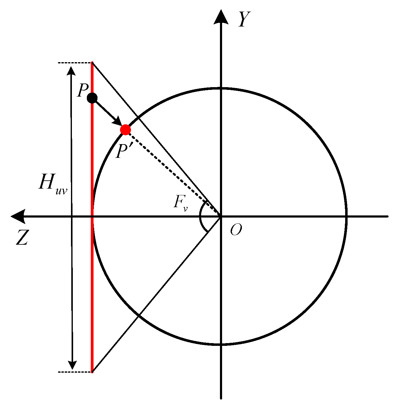
2.2. Perspective Projection

When perspective (i.e., rectilinear) projection [33] is used in the procedure to render a VP, the cross-section of the UV plane and the sphere can be represented as in Figure 3, where point P is projected onto P along the straight line between O and P . In this case, the width W u v and height H u v of the UV plane depend on the horizontal and vertical FOVs, respectively, as follows:
W u v = 2 tan ( F h 2 )
H u v = 2 tan ( F v 2 )
where F h and F v denote the FOVs in the horizontal and vertical directions, respectively. By applying (12) and (13), the function f M ( m ,   n ) of (6) is represented by the following equations for the perspective projection [33].
u = ( m + 0 . 5 ) W u v W V P ,   0   m   < W V P
v = ( n + 0.5 ) H u v H V P ,   0   n   < H V P
where W V P and H V P are the width and height of the VP, respectively. The position ( u,v ) of P in Figure 3 is represented with 3D coordinates ( x ,   y ,   z ) using the geometric structure as follows:
[ x y z ] = [ 1 0 0 1 0 0 ] [ u v ] + [ W u v / 2 H u v / 2 1 ]
Point P is projected onto point P on the unit sphere, where the coordinates ( X , Y , Z ) of P can be determined as follows:
X = x x 2 + y 2 + z 2
Y = y x 2 + y 2 + z 2
Z = z x 2 + y 2 + z 2
Equations (16)–(19) explain the detailed procedure of f p ( u ,   v ) in (7) when the perspective projection [33] is used.

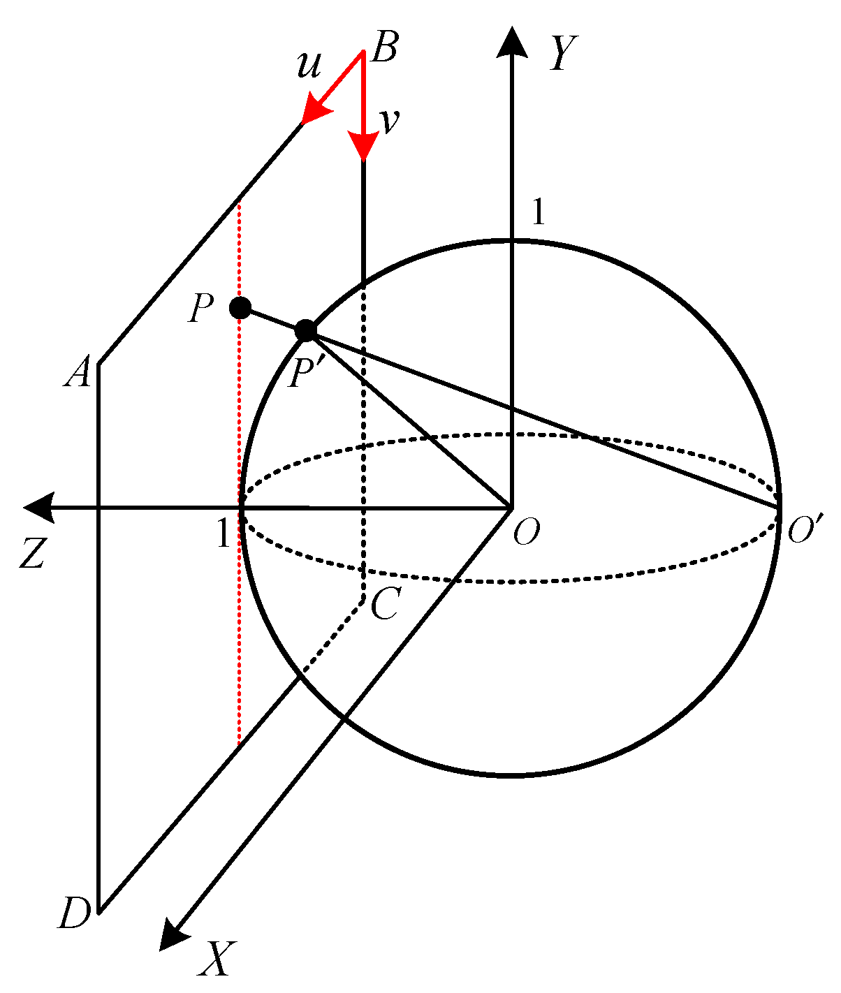
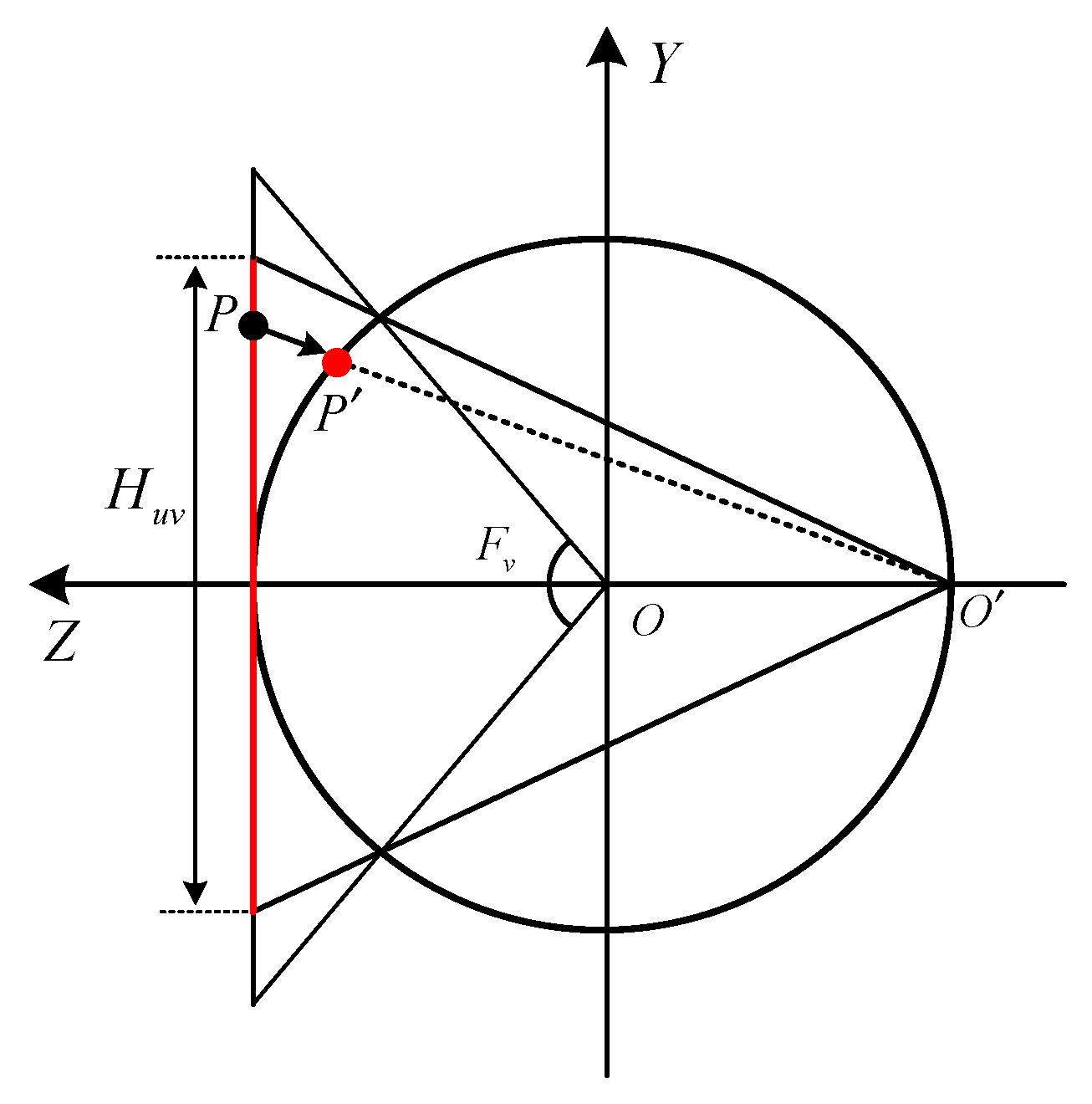
2.3. Stereographic Projection

Figure 4 shows the UV plane and sphere when the stereographic projection [33] is used, where point P is projected onto P along the straight line between O and P , whereas the line between O and P is used in the perspective projection [33].
The cross-section of Figure 4 is shown in Figure 5, where the width W u v and height H u v of the UV plane can be determined as follows:
W u v = 4 sin ( F h 2 ) 1 + cos ( F h 2 )
H u v = 4 sin ( F v 2 ) 1 + cos ( F v 2 )
In the stereographic projection, f M ( m ,   n ) from (6) is implemented by substituting (20) and (21) into (14) and (15). After ( u ,   v ) has been derived by using f M ( m ,   n ) , it can be represented with 3D coordinates ( x ,   y ,   z ) by applying (16). When the stereographic projection is used, the 3D coordinates of P are as follows:
X = 4 x x 2 + y 2 + 4
Y = 4 y x 2 + y 2 + 4
Z = 8 x 2 + y 2 + 4 + 1

3. Limitation of the Conventional Methods

According to Jabar et al. [24], the conventional algorithms that are used to render the viewport produce a variety of distortions when the FOV is wide, although these distortions may not be noticeable for narrow FOVs. In this section, we discuss the reasons why the conventional techniques have limitations for wide FOVs followed by the analysis of the degradation tendency according to the degree of the FOV.

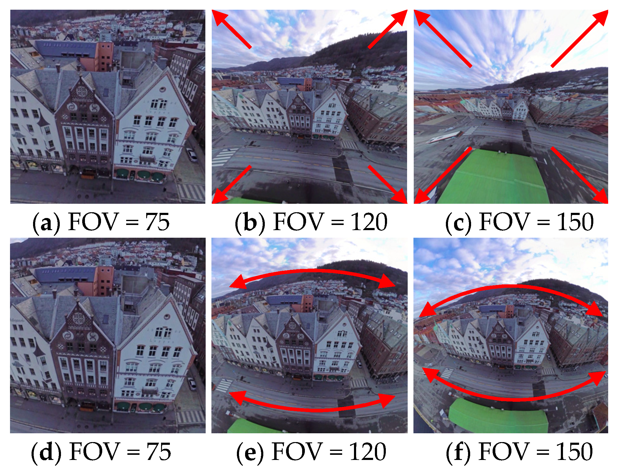
3.1. Distortions in Conventional Methods

The subjective qualities of the viewports that are generated with various FOVs are compared in Figure 6, where (a–c) and (d–f) show the perspective [33] and stereographic [33] projections, respectively. As observed in Figure 6, when the perspective projection is used, the viewport shows a distorted perspective for a wide FOV. On the other hand, when the stereographic projection is used, straight lines are severely bent as the FOV increases.

3.2. Analysis of the Distortion Resulting from Conventional Methods

As illustrated in Figure 2, the pixel values in the viewport are set to those with the corresponding P points on the unit sphere. When the pixel value at ( m ,   n ) in the VP is denoted by I ( m ,   n ) , the corresponding P point on the unit sphere is represented by P ( m , n ) , where the coordinate of P ( m , n ) is denoted with the form ( X ( m , n ) , Y ( m , n ) , Z ( m , n ) ) . To analyze the distance between the positions of the corresponding P ( m , n ) points, we calculated the vertical length of the arc between P ( m , n ) and P ( m , n + 1 ) and the horizontal length between P ( m , n ) and P ( m + 1 , n ) , as demonstrated in Figure 7. Note that the length is the sampling interval that is used to generate a VP from a 360° image.
In Figure 7, d h ( m ,   n ) = | P ( m , n ) P ( m + 1 , n ) ¯ | and l h ( m ,   n ) = | P ( m , n ) P ( m + 1 , n ) | are the shortest direct distance and the length of the arc between the horizontally nearest P ( m , n ) neighbors. Similarly,   d v ( m ,   n ) and l v ( m ,   n ) are the values for the vertically nearest neighbors, respectively, as follows:
d h ( m ,   n * ) = | P ( m , n * ) P ( m + 1 , n * ) ¯ | = ( X ( m , n * ) X ( m + 1 , n * ) ) 2 + ( Y ( m , n * ) Y ( m + 1 , n * ) ) 2 + ( Z ( m , n * ) Z ( m + 1 , n * ) ) 2
d v ( m * ,   n ) = | P ( m * , n ) P ( m * , n + 1 ) ¯ | = ( X ( m * , n ) X ( m * , n + 1 ) ) 2 + ( Y ( m * , n ) Y ( m * , n + 1 ) ) 2 + ( Z ( m * , n ) Z ( m * , n + 1 ) ) 2
l h ( m   , n * ) = | P ( m , n * ) P ( m + 1 , n * ) | = 2 sin 1 ( d h ( m , n * ) 2 )
l v ( m * , n ) = | P ( m * , n ) P ( m * , n + 1 ) | = 2 sin 1 ( d v ( m * , n ) 2 )
where 0   m   < W V P 1 , 0   n   < H V P 1 , n * and m * are the specific values that are used to calculate the lengths of the arcs between the horizontal and vertical positions. Figure 8 presents the normalized values of l h ( m ,   n * ) according to the horizontal FOV ( F h ) when the perspective and stereographic projections are used. In this figure, we can observe that the length between the locations of the consecutive sampling points on the sphere decreases as m moves away from the center ( m = ( W V P / 2 ) 1 ). This means that the pixels in the boundary region of a VP are made by sampling the P points with reduced sampling intervals on the sphere. This makes the pixels in the VP look like a stretched form of P points on the sphere. This tendency is more significant as F h increases. As observed in Figure 8a,b, the amount of stretching in the perspective projection is greater than that in the stereographic projection. Note that the analysis for l v ( m * , n ) is similar to those in Figure 8, although it is not presented in this paper.

4. Algorithm Proposed to Render the Viewport

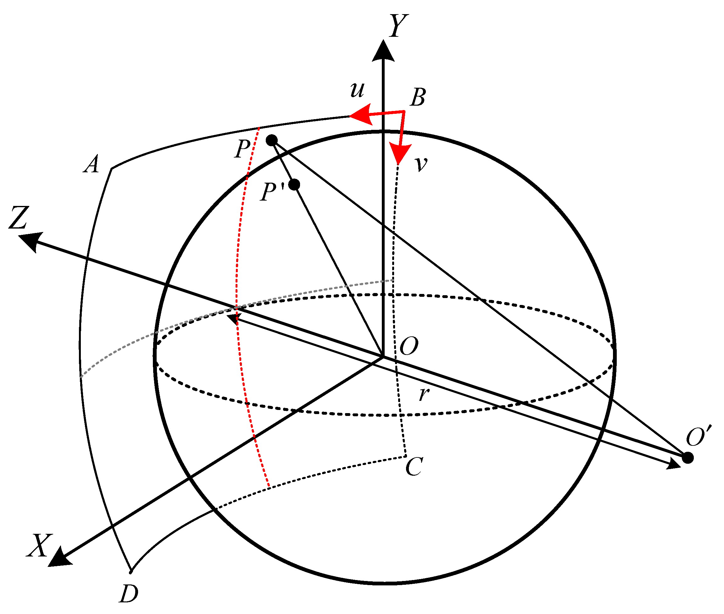
4.1. Curved UV Surface

By analyzing Figure 8 in the previous section, when the VP is rendered with the wide FOV, the degradation in the VP is due to the non-uniformed sampling space. In this section, we propose a model for the UV surface, which makes the sampling space uniform. Figure 9 depicts a model to represent the proposed UV surface, which is tangent to the unit sphere. The proposed UV surface is a part of the outer sphere whose center and radius are O and r , respectively. The outer sphere intersects with the unit sphere at the center of the UV surface. The outer sphere is represented by the following equation.
x 2 + y 2 + ( z + r 1 ) 2 = r 2
In Figure 10, the red curve represents the cross-section of the proposed UV surface, where F v is the vertical FOV and F v O U T is the corresponding vertical angle at the center O of the outer sphere to cover the surface that is generated by applying F v at the center O of the unit sphere. The relationship between F v and F v O U T is as follows:
tan ( F v 2 ) = r   sin ( F v O U T 2 ) r   cos ( F v O U T 2 ) ( r 1 )
Equation (30) can be rewritten as follows:
F v O U T = 4 tan 1 ( r 2 + ( 2 r 1 ) tan 2 ( F v 2 ) r ( 2 r 1 ) tan ( F v 2 ) )
u = m + 0 . 5 W V P , 0   m   < W V P
v = n + 0 . 5 H V P , 0   n   < H V P
Note that Equation (31) is numerically stable only for r > 0.5 . F v O U T   has a complex number for 0 < r < 0.5 . When r = 0.5 , F v O U T is not defined. However, because the curved UV surface is a part of the outer sphere as shown in Figure 10, r would be larger than 1. Thus, in the proposed algorithm, F v O U T   is always numerically stable.
Equations (32) and (33) explain the detailed process for f M ( m ,   n ) from (6) when the proposed UV surface is used. Based on the geometry that is related to the outer sphere, the coordinates ( x ,   y ,   z ) of P are derived as follows:
ϕ O U T = F h O U T × ( 0 . 5 u )
θ O U T = F v O U T × ( 0 . 5 v )
x = r   cos ( θ O U T ) sin ( ϕ O U T )
y = r   sin ( θ O U T )
z = r   cos ( θ O U T ) cos ( ϕ O U T ) ( r 1 )
Point P is projected onto point P on the unit sphere, where the coordinates of P are ( X , Y , Z ) , which are calculated by using (17)–(19). When the proposed UV surface is used, f p ( u ,   v ) from (7) is implemented by applying (34)–(38) and (17)–(19).
Figure 11 displays the VPs that occur from applying the curved UV surface for the FOV = {75, 120} and r = {2, 5, 20, 0.3}, where a larger outer sphere produces flatter straight lines. When r is set to 0.3, the generated viewports degrade significantly, because r = 0.3 is included in the range of instability in Equation (31).

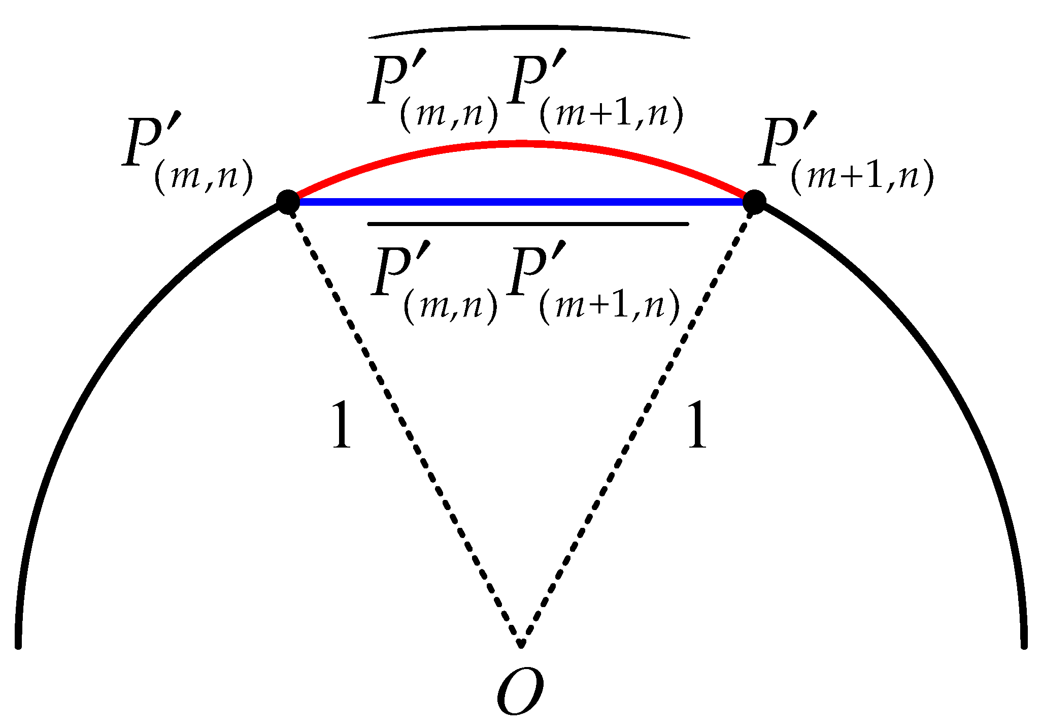
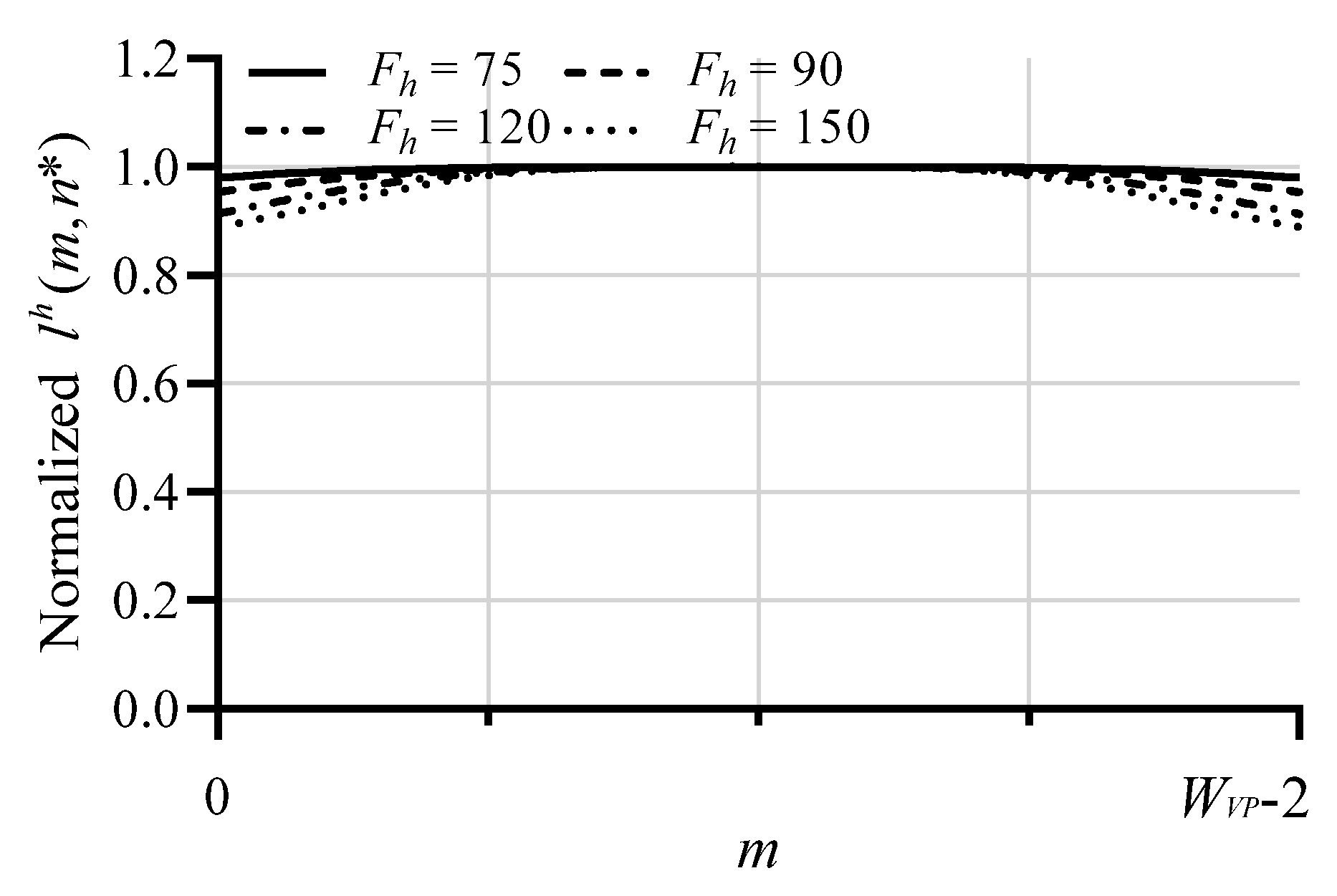
4.2. Adjusted Sampling Intervals

In this section, we adjust the sampling intervals that are made by using the curved UV surface so that the sampling positions are more evenly spaced. Figure 12 presents a mapping function between the original index u and the modified index u on the UV plane, where the function passes through {S(1), S(3), S(5)} on the diagonal line and {S(2), S(4)}, which are not on the diagonal line. {S(1), S(2), S(3), S(4), S(5)} are ancillary parameters that are used to explain the mapping function. The quantity of the deviation of {S(2), S(4)} from the diagonal line is set to w , which is defined as follows:
w = FOV thr FOV α ,   FOV     thr FOV
where thr FOV is a threshold for the FOV. When the FOV is larger than thr FOV , i.e., when the FOV is wide, the sampling intervals are modified. In (39), the parameter α is set based on the empirical data. Using this mapping function, the sampling points P on the unit sphere are more uniformly sampled horizontally. This reduces the degradation (e.g., stretching) in the boundary regions of the viewport.
The mapping function in Figure 12 can be modeled with the following equation:
u = g ( u ) = c 0 + c 1 u + c 2 u 2 + c 3 u 3
where the variables { c 0 , c 1 , c 2 , c 3 } are calculated by applying a polynomial regression algorithm [34] as follows:
[ u 1 u 2 u 3 u 4 u 5 ] = [ 1 u 1 u 1 2 u 1 3 1 u 2 u 2 2 u 2 3 1 u 3 u 3 2 u 3 3 1 u 4 u 4 2 u 4 3 1 u 5 u 5 2 u 5 3 ] [ c 0 c 1 c 2 c 3 ]
u = U c
c = ( U T U ) 1 U T u
Note that all of the techniques that are explained in this subsection can be applied for v .
In Figure 8a,b, if the sampling positions are ideal, then the normalized l h ( m , n * ) is equal to 1 for all m values. Thus, the degradations in these figures can be evaluated by using the following equation.
L n * h = 1 W V P 1 m = 0 W V P 2 { 1 ( l h ( m , n * ) Max ( l h ( m , n * ) ) ) } 2
In order to analyze the effect of the parameter r of equation (29) in the proposed algorithm, the values of L n * h of (44) for various   r are shown in Figure 13. In the figure, as the value of L n * h decreases, the quality of the viewport increases because it means that the data on the sphere are sampled uniformly. As shown in Figure 13, the optimal values of r differ based on F h , where the optimal values of r for F h = {75, 90, 120, 150} are {3.2061, 3.4041, 3.1588, 2.9040}, respectively. The optimal values for r were obtained by Quasi-Newton Method [35].
To demonstrate the effect of the proposed UV surface, Figure 14 displays the normalized l h ( m , n * ) when ( u ,   v ) of the UV plane is modified by applying the mapping technique of Figure 12 for u and v independently after the proposed UV surface is employed with the optimized values of r .
Based on (44), the degradations of the various methods in Figure 8 and Figure 14 are summarized in Table 1. As observed in Table 1, the degradation of the proposed algorithm is much smaller than those for conventional algorithms. The degradation values in the r = 0.3 column are larger than those in other columns because r = 0.3 is one instance of invalid data. The analysis for l v ( m , n * ) is similar to those in Figure 8 and Figure 14, although it is not provided in this manuscript.

5. Simulation Results

To demonstrate the performance of the proposed algorithm, we compared it with a variety of conventional techniques, including the perspective projection [33], stereographic projection [33], Pannini projection [25], automatic content-aware (ACA) projection [27], and adaptive cylindrical (AC) projection [32].

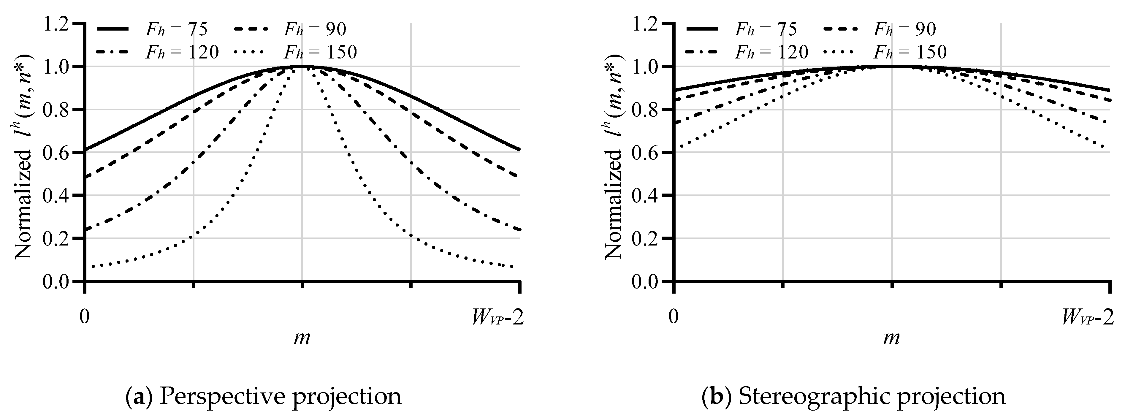
5.1. Quantitative Evaluation

In this section, an objective evaluation is performed for the various conventional techniques and the proposed algorithm, where straightness and conformality are used as criteria, as demonstrated by Kim et al. [27]. Figure 15 explains how to calculate the straightness and conformality as criteria in the objective evaluation. The evaluation equations for these are as follows:
Straightness = α 2 α 1 + α 2 .
Conformality = min ( β 1 , β 2 , β 3 , β 4 ) max ( β 1 , β 2 , β 3 , β 4 )
The maximum values of straightness and conformality are 1. As these values get closer to 1, the degradation in the straightness and conformality decreases.
Figure 16 displays the patterns that occur using the various algorithms when nested squares are used as a test pattern to evaluate the straightness and conformality. It can be observed that some lines are curved and some red circles have been deformed. The bent lines imply that the applied methods result in poor performance with respect to the straightness. In a case where the circle is badly deformed, we know that the conformality of the algorithm is not good.
Based on (45) and (46), the evaluation results for the straightness and conformality are summarized in Table 2, where the best results and the second-best results are represented with red and blue numbers, respectively.
As observed in Figure 16 and Table 2, the perspective method shows the best performance in the straightness, whereas it provides one of the worse results for the conformality. In contrast, the stereographic method shows the smallest value for the straightness and the largest value for the conformality. This implies that the stereographic algorithm outperforms the other techniques in maintaining the shape of the circles in the viewport, but it bends the lines more than the other schemes. Although the proposed algorithm does not provide the best performance for the straightness and conformality, the overall performance of the proposed algorithm is in the upper ranks. In particular, Figure 16 shows that the overall subjective deformation is much less than the other techniques.

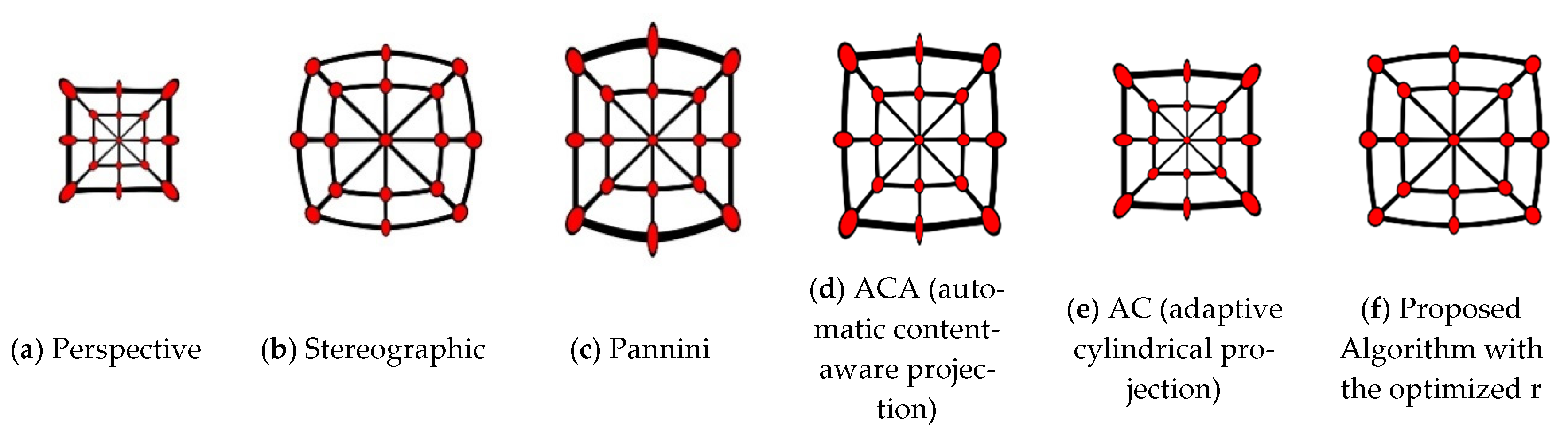
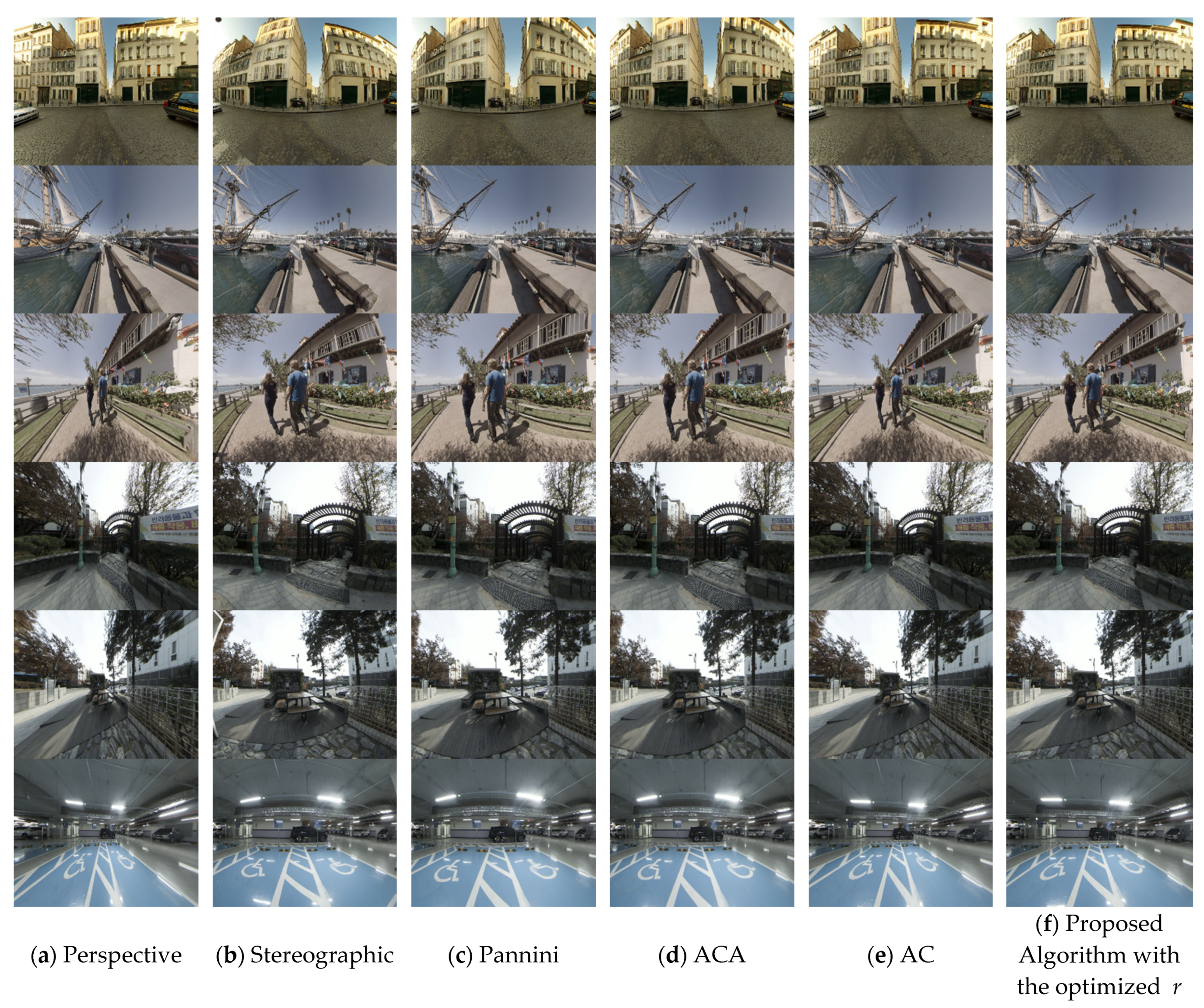
5.2. Qualitative Evaluation

In this section, we evaluate the subjective performances of the various algorithms that are used to render a viewport picture. Figure 17 presents the six test images that are used for the subjective evaluation, which show the equirectangular images whose horizontal and vertical FOVs are 360° × 180°, respectively.
Figure 18 displays the viewport images that are rendered by the various projection methods. The viewport images rendered by the equirectangular pictures are shown in Figure 18 in which the horizontal and vertical FOVs of the viewport are set to 150° and 120°, respectively. As demonstrated in Figure 18, the subjective qualities of the proposed method are much higher than those of the others. This is because the objects are deformed and the lines are bent in the pictures that are produced by the perspective [33], stereographic [33], Pannini [25], ACA [27] and, AC [32] methods.

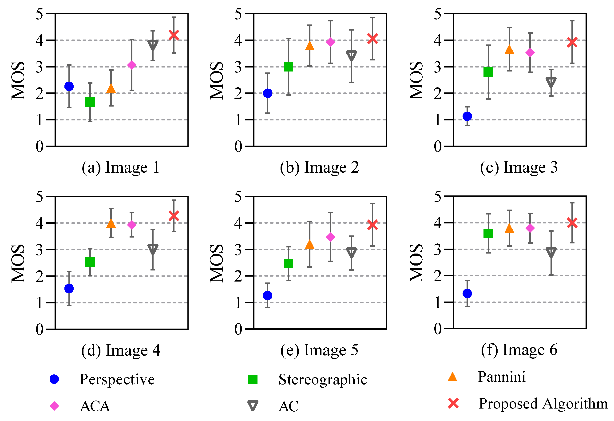
5.3. Perceptual Evaluation

To provide simulation results for the perceptual evaluation, the single stimulus method of BT.500 [36] is used for the images in Figure 19. The mean opinion score (MOS) is a simple measurement to obtain the viewers’ opinions. The MOS provides a numerical indication of the quality that is perceived by the viewers. The MOS is expressed as a single number in the range of 1–5, where 1 means bad and 5 means excellent. In this test, the viewport images with a wide FOV were evaluated and they were scored by 20 viewers who were graduate students. Figure 19 shows the MOS values. The MOS values of the proposed method are always much higher than those of the conventional methods [25,27,31,33].

5.4. Complexity Comparision

To compare the computational complexities of the algorithms, we evaluated the central processing unit (CPU) times that were required by the various algorithms, where a personal computer incorporating an AMD Ryzen 5 2600 six-core Processor @3.40 GHz and DDR4 32 GB was used. The CPU times are summarized in Table 3, where the proposed algorithm is much simpler than ACA [27]. This is because ACA [27] required additional processes to detect the line component and to optimize the related parameter, whereas the proposed algorithm does not need these. The complexities of the other conventional algorithms, such as the perspective [33], stereographic [33], Pannini [25], and AC [32] algorithms are approximately equal to that of the proposed method.

6. Conclusions

We discussed the limitations of the conventional algorithms that are used to render the VP and we have proposed an algorithm to overcome these problems. A curved surface was used to efficiently project the pixel data on the unit sphere of an omnidirectional visual system onto the VP. Even though conventional techniques use a flat square plane to project the pixel data with non-uniform sampling intervals, the proposed curved surface reduced the non-uniformity and this resulted in a perceptually enhanced VP.
Using rendering engines can be considered to implement the proposed algorithm in real-time applications. First, the rasterization-based pipeline in the GPU is a unit designed to increase the speed of filling the pixel values in the triangle meshes on the screen. However, the proposed algorithm projects a value on the sphere to the pixel in the viewport. Consequently, the proposed algorithm is not suitable for implementation using the rasterization-based pipeline in the GPU. Second, the ray tracing-based pipeline in the GPU can be considered to enhance the algorithm’s performance. In this scenario, we need to access the data pixel-by-pixel in the module of the ray-tracing pipeline. However, most commercial GPU products do not provide the accessibility. Third, we can consider Intel Embree, which is a collection of high-performance ray tracing kernels. Since the Embree does not have the limitations of GPU-based systems, it best matches the proposed algorithm.

Author Contributions

Conceptualization, G.-W.L. and J.-K.H.; Data curation, G.-W.L.; Formal analysis, G.-W.L.; Funding acquisition, J.-K.H.; Investigation, G.-W.L.; Methodology, G.-W.L. and J.-K.H.; Software, G.-W.L.; Supervision J.-K.H.; Visualization, G.-W.L. and J.-K.H.; Writing—review & editing, J.-K.H. All authors have read and agreed to the published version of the manuscript.

Funding

This work was partially supported by the National Research Foundation of Korea (NRF) under Grant NRF-2018R1A2A2A05023117 and partially supported by the Institute for Information & Communications Technology Promotion (IITP) under Grant 2017-0-00486 funded by the Korea government (MSIT).

Institutional Review Board Statement

Not applicable.

Informed Consent Statement

Not applicable.

Data Availability Statement

The data presented in this study are available on request from the corresponding author.

Conflicts of Interest

The authors declare no conflict of interest. The funders had no role in the design of the study; in the collection, analyses, or interpretation of data; in the writing of the manuscript, or in the decision to publish the results.

References

  1. Bauermann, I.; Mielke, M.; Steinbach, E.H. 264 based coding of omnidirectional video. In Proceedings of the International Conference on Computer Vision and Graphics, Warsaw, Poland, 22–24 September 2004; Volume 32. [Google Scholar]
  2. Kuzyakov, E.; Pio, D. Next-Generation Video Encoding Techniques for 360 Video and vr. Blogpost, January 2016. Available online: https://code.facebook.com/posts/1126354007399553 (accessed on 18 December 2020).
  3. Hosseini, M.; Swaminathan, V. Adaptive 360 VR video streaming: Divide and conquer. In Proceedings of the 2016 IEEE International Symposium on Multimedia (ISM), San Jose, CA, USA, 11–13 December 2016; pp. 107–110. [Google Scholar]
  4. Smus, B. Three Approaches to VR Lens Distortion. 2016. Available online: http://smus.com/vr-lens-distortion/ (accessed on 18 December 2020).
  5. Champel, M.-L.; Koenen, R.; Lafruit, G.; Budagavi, M. Draft 1.0 of ISO/IEC 23090-1: Technical Report on Architectures for Immersive Media, Document N17741, ISO/IEC JTC1/SC29/WG11. In Proceedings of the 123rd Meeting, Ljubljana, Slovenia, 16–20 July 2018. [Google Scholar]
  6. Bross, B.; Chen, J.; Liu, S. Versatile Video Coding (Draft 6). In Proceedings of the 15th Meeting Joint Video Exploration Team (JVET), Document JVET-O2001, Gothenburg, Sweden, 12 July 2019. [Google Scholar]
  7. Ye, Y.; Boyce, J. Algorithm descriptions of projection format conversion and video quality metrics in 360Lib Version 8. In Proceedings of the 12th Meeting Joint Video Exploration Team (JVET), Document JVET-L1004, Macau, China, 3–12 October 2018. [Google Scholar]
  8. Szeliski, R. Image Alignment and Stitching: A Tutorial; Foundations and Trends® in Computer Graphics and Vision, Vol.2: No.1; Now Publishers Inc.: Hanover, MA, USA, 2007; pp. 1–104. [Google Scholar] [CrossRef]
  9. Zaragoza, J.; Chin, T.; Tran, Q.; Brown, M.S.; Suter, D. As-Projective-As-Possible Image Stitching with Moving DLT. In Proceedings of the IEEE Transactions on Pattern Analysis and Machine Intelligence, Portland, OR, USA, 23–28 June 2013; Volume 36, no. 7. pp. 1285–1298. [Google Scholar]
  10. Li, J.; Wang, Z.; Lai, S.; Zhai, Y.; Zhang, M. Parallax-Tolerant Image Stitching Based on Robust Elastic Warping. IEEE Trans. Multimed. 2018, 20, 1672–1687. [Google Scholar] [CrossRef]
  11. Zheng, J.; Wang, Y.; Wang, H.; Li, B.; Hu, H. A Novel Projective-Consistent Plane Based Image Stitching Method. IEEE Trans. Multimed. 2019, 21, 2561–2575. [Google Scholar] [CrossRef]
  12. Triggs, B.; McLauchlan, P.F.; Hartley, R.I.; Fitzgibbon, A.W. Bundle adjustment a modern synthesis. In Vision Algorithms: Theory and Practice; Springer: New York, NY, USA, 2000; pp. 298–372. [Google Scholar]
  13. Lourakis, M.I.; Argyros, A.A. SBA: A software package for generic sparse bundle adjustment. ACM Trans. Math. Softw. 2009, 36, 1–30. [Google Scholar] [CrossRef]
  14. Burt, P.; Adelson, E.H. A Multiresolution Spline with Application to Image Mosaics. ACM Trans. Graph. 1983, 2, 217–236. [Google Scholar] [CrossRef]
  15. Agarwala, A. Efficient gradient-domain compositing using quadtrees. ACM Trans. Graph. 2007, 26, 94. [Google Scholar] [CrossRef]
  16. Greene, N. Environment Mapping and Other Applications of World Projections. IEEE Comput. Graph. Appl. 1986, 6, 21–29. [Google Scholar] [CrossRef]
  17. Snyder, J.P. Flattening the Earth: Two Thousand Years of Map Projections; Univ. Chicago Press: Chicago, IL, USA, 1993; pp. 5–8. [Google Scholar]
  18. Hanhart, P.; Xiu, X.; He, Y.; Ye, Y. 360° Video Coding Based on Projection Format Adaptation and Spherical Neighboring Relationship. IEEE J. Emerg. Sel. Top. Circuits Syst. 2019, 9, 71–83. [Google Scholar] [CrossRef]
  19. Lin, J.L.; Lee, Y.H.; Shih, C.H.; Lin, S.Y.; Lin, H.C.; Chang, S.K.; Wang, P.; Liu, L.; Ju, C.C. Efficient Projection and Coding Tools for 360° Video. IEEE J. Emerg. Sel. Top. Circuits Syst. 2019, 9, 84–97. [Google Scholar] [CrossRef]
  20. Song, J.; Yang, F.; Zhang, W.; Zou, W.; Fan, Y.; Di, P. A Fast FoV-Switching DASH System Based on Tiling Mechanism for Practical Omnidirectional Video Services. IEEE Trans. Multimed. 2020, 22, 2366–2381. [Google Scholar] [CrossRef]
  21. Tang, M.; Wen, J.; Zhang, Y.; Gu, J.; Junker, P.; Guo, B.; Jhao, G.; Zhu, Z.; Han, Y. A Universal Optical Flow Based Real-Time Low-Latency Omnidirectional Stereo Video System. IEEE Trans. Multimed. 2019, 21, 957–972. [Google Scholar] [CrossRef]
  22. Fan, X.; Lei, J.; Fang, Y.; Huang, Q.; Ling, N.; Hou, C. Stereoscopic Image Stitching via Disparity-Constrained Warping and Blending. IEEE Trans. Multimed. 2020, 22, 655–665. [Google Scholar] [CrossRef]
  23. Yu, M.; Lakshman, H.; Girod, B. A framework to evaluate omnidirectional video coding schemes. In Proceedings of the 2015 IEEE International Symposium on Mixed and Augmented Reality, Fukuoka, Japan, 29 September–3 October 2015; pp. 31–36. [Google Scholar]
  24. Jabar, F.; Ascenso, J.; Queluz, M.P. Perceptual analysis of perspective projection for viewport rendering in 360° images. In Proceedings of the 2017 IEEE International Symposium on Multimedia (ISM), Taichung, Taiwan, 11–13 December 2017; pp. 53–60. [Google Scholar]
  25. Sharpless, T.K.; Postle, B.; German, D.M. Pannini: A new projection for rendering wide angle perspective images. In Proceedings of the Sixth International Conference on Computational Aesthetics in Graphics, London, UK, 14–15 June 2010; pp. 9–16. [Google Scholar]
  26. Weisstein, E.W. Cylindrical Projection. From MathWorld—Wolfram Web Resource. Available online: http://mathworld.wolfram.com/CylindricalProjection.html (accessed on 18 December 2020).
  27. Kim, Y.W.; Lee, C.R.; Cho, D.Y.; Kwon, Y.H.; Choi, H.J.; Yoon, K.J. Automatic content-aware projection for 360 videos. In Proceedings of the 2017 IEEE International Conference on Computer Vision (ICCV), Venice, Italy, 22–29 October 2017; pp. 4753–4761. [Google Scholar]
  28. Kopf, J.; Lischinski, D.; Deussen, O.; Cohen-Or, D.; Cohen, M. Locally Adapted Projections to Reduce Panorama Distortions. In Computer Graphics Forum; Blackwell Publishing Ltd.: Oxford, UK, 2009; Volume 28, pp. 1083–1089. [Google Scholar]
  29. Tehrani, M.A.; Majumder, A.; Gopi, M. Correcting perceived perspective distortions using object specific planar transformations. In Proceedings of the 2016 IEEE International Conference on Computational Photography (ICCP), Evanston, IL, USA, 13–15 May 2016; pp. 1–10. [Google Scholar]
  30. Jabar, F.; Ascenso, J.; Queluz, M.P. Content-aware perspective projection optimization for viewport rendering of 360° images. In Proceedings of the 2019 IEEE International Conference on Multimedia and Expo (ICME), Shanghai, China, 8–12 July 2019; pp. 296–301. [Google Scholar]
  31. Hou, X.; Zhang, L. Saliency detection: A spectral residual approach. In Proceedings of the 2007 IEEE Conference on Computer Vision and Pattern Recognition, Minneapolis, MN, USA, 17–22 June 2007; pp. 1–8. [Google Scholar]
  32. Kopf, J.; Uyttendaele, M.; Deussen, O.; Cohen, M.F. Capturing and viewing gigapixel images. ACM Trans. Graph. 2017, 26, 93-es. [Google Scholar] [CrossRef]
  33. Snyder, J.P. Map Projections—A Working Manual; US Government Printing Office: Washington, DC, USA, 1987.
  34. Weisstein, E.W. Least Squares Fitting-Polynomial. From MathWorld—A Wolfram Web Resource. Available online: http://mathworld.wolfram.com/LeastSquaresFittingPolynomial.html (accessed on 18 December 2020).
  35. Shanno, D.F. Conditioning of quasi-Newton methods for function minimization. Math. Comput. 1970, 24, 647–656. [Google Scholar] [CrossRef]
  36. Int. Telecommun. Union Methodology for the Subjective Assessment of the Quality of Television Pictures ITU-R Recommendation BT.500-14; International Telecommunication Union: Geneva, Switzerland, 2019. [Google Scholar]
Figure 1. 3D XYZ coordinates used to describe the pixel location in the 360° image.
Applsci 11 01133 g001
Figure 2. Procedure to render the viewport from the 360° image.
Applsci 11 01133 g002
Figure 3. Cross-section of the UV plane and sphere when the perspective projection is used.
Applsci 11 01133 g003
Figure 4. UV plane and sphere when the stereographic projection is used.
Applsci 11 01133 g004
Figure 5. Cross-section of the UV plane and sphere when the stereographic projection is used.
Applsci 11 01133 g005
Figure 6. Distortions resulting from the perspective projection [33] (ac) and stereographic projection [33] (df).
Applsci 11 01133 g006
Figure 7. Cross-section of the sphere to explain the shorter direct distance and the distance following the curved surface between P ( m , n ) and P ( m + 1 , n ) .
Applsci 11 01133 g007
Figure 8. Normalized l h ( m   , n * ) when n * = H V P / 2 .
Applsci 11 01133 g008
Figure 9. Curved UV surface, which is the tangent surface for the unit sphere.
Applsci 11 01133 g009
Figure 10. Cross-section of the proposed UV surface and the unit sphere.
Applsci 11 01133 g010
Figure 11. Viewport pictures (VPs) resulting from applying the curved UV surface.
Applsci 11 01133 g011
Figure 12. Adjustment function to modify the sampling position on the UV plane.
Applsci 11 01133 g012
Figure 13. L n * h of (44) for various r and F h in the proposed algorithm.
Applsci 11 01133 g013
Figure 14. Normalized l h ( m , n * = H V P / 2 ) when the proposed UV surface is used with the optimized values of r and u is modified by the mapping function g ( u ) .
Applsci 11 01133 g014
Figure 15. Straightness and conformality as the criteria in the quantitative evaluation.
Applsci 11 01133 g015
Figure 16. Test patterns produced by the various algorithms.
Applsci 11 01133 g016
Figure 17. Test images: six equirectangular images where the horizontal and vertical FOVs are 360° × 180°, respectively.
Applsci 11 01133 g017
Figure 18. Viewport images produced by various projection techniques for the equirectangular test images of Figure 17.
Applsci 11 01133 g018
Figure 19. Mean opinion score (MOS) values of the viewport images shown in Figure 18.
Applsci 11 01133 g019
Table 1. Degradation evaluated with (44) for the various techniques.
F h . Perspective
Projection
Stereographic
Projection
Curved UV
Surface   with   the   Optimized   r
Curved UV
Surface with r = 0.3
750.0396040.0026970.0000100.173255
900.0787990.0055040.0000510.335975
1200.2294150.0167790.0002890.559911
1500.5176750.0395230.0007010. 597737
Table 2. Quantitative evaluation of the projection results.
Projection MethodStraightnessConformality
Perspective [33]0.9999990.719107
Stereographic [33]0.9735220.878603
Pannini [25]0.977370.788848
ACA [27]0.9780320.753724
AC [32]0.9786400.616209
Proposed Algorithm
with the optimized r
0.9805970.826667
Table 3. Central processing unit (CPU) time consumed by the various algorithms.
Projection MethodConsumed CPU Time (Second)
Perspective [33]0.201
Stereographic [33]0.241
Pannini [25]0.270
ACA [27]1.066
AC [32]0.253
Proposed Algorithm
with the optimized r
0.340
Publisher’s Note: MDPI stays neutral with regard to jurisdictional claims in published maps and institutional affiliations.

