Article

Towards TBM Automation: On-The-Fly Characterization and Classification of Ground Conditions Ahead of a TBM Using Data-Driven Approach

by
Sylvanus Sebbeh-Newton
1,*,
Prosper E.A. Ayawah
2,
Jessica W.A. Azure
3,
Azupuri G.A. Kaba
4,
Fauziah Ahmad
5,
Zurinahni Zainol
6 and
Hareyani Zabidi
1,*
1
School of Materials and Mineral Resources Engineering, Universiti Sains Malaysia, Penang 14300, Malaysia
2
Geological Engineering Department, Missouri University of Science and Technology, Rolla, MO 65409, USA
3
Mining Engineering Department, Missouri University of Science and Technology, Rolla, MO 65409, USA
4
John Wood Group, Geotechnical Department, Albuquerque, NM 87113, USA
5
School of Civil Engineering, Universiti Sains Malaysia, Penang 14300, Malaysia
6
School of Computer Sciences, Universiti Sains Malaysia, Penang 11800, Malaysia
*
Authors to whom correspondence should be addressed.
Appl. Sci. 2021, 11(3), 1060; https://doi.org/10.3390/app11031060
Submission received: 1 December 2020 / Revised: 28 December 2020 / Accepted: 30 December 2020 / Published: 25 January 2021

Abstract

:
Pre-tunneling exploration for rock mass classification is a common practice in tunneling projects. This study proposes a data-driven approach that allows for rock mass classification. Two machine learning (ML) classification models, namely random forest (RF) and extremely randomized tree (ERT), are employed to classify the rock mass conditions encountered in the Pahang-Selangor Raw Water Tunnel in Malaysia using tunnel boring machine (TBM) operating parameters. Due to imbalance of rock classes distribution, an oversampling technique was used to obtain a balanced training dataset for unbiased learning of the ML models. A five-fold cross-validation approach was used to tune the model hyperparameters and validation-set approach was used for the model evaluation. ERT achieved an overall accuracy of 95%, while RF achieved 94% accuracy, in rightly classifying rock mass conditions. The result shows that the proposed approach has the potential to identify and correctly classify ground conditions of a TBM, which allows for early problem detection and on-the-fly support system selection based on the identified ground condition. This study, which is part of an ongoing effort towards developing reliable models that could be incorporated into TBMs, shows the potential of data-driven approaches for on-the-fly classification of ground conditions ahead of a TBM and could allow for the early detection of potential construction problems.

1. Introduction

Tunnel boring machines (TBMs) are currently the most utilized equipment for deep and long tunnels in both civil and mining industries. One important consideration prior to the actual excavation is evaluating ground conditions along the proposed tunnel alignment. This initial evaluation provides critical information for selecting the excavation type and developing preliminary ground support systems. Ground conditions are obtained by the characterization and subsequent classification of the rock mass based on a pre-defined system known as a rock mass classification system. Since the introduction of rock mass classification by Terzaghi, it has become a useful tool for rock engineering and is widely considered the most practical method for evaluating the quality of the rock mass in underground engineering practices. The common and widely used classification systems are the Q-system [1], Rock Mass Rating (RMR) [2], Rock Mass Index (RMi) [3], and Geological Strength Index (GSI) [4]. Aside from these classification systems, the Japanese Highway Classification System (JH system) and the Hydropower Classification System (HC system) are also popular in Asia.
One of the serious concerns in the use of rock mass classifications schemes is that they are subjective. Field engineers with different experience levels classifying the same rock mass using for example, RMR, can produce significantly different rock mass behavior [5]. This is because most of these classification systems use both quantitative and qualitative methodologies. To reduce, if not to eliminate, the subjectivity or experience factor in rock mass classification, a data-driven system is necessary. Some of the early attempts on data-driven approaches focused on the use of non-destructive forward geological prospecting techniques including tunnel seismic prediction (TSP), and ground penetration radar (GPR) to assess the rock mass quality ahead of TBMs [6,7]. Although these geophysical techniques provide reliable and accurate results, they are expensive and cause undue project delays. Zhang et al. [8] indicated that these forward geophysical prospecting techniques are not directly related to the rock tunneling/excavation process since they can only be implemented when the TBM is not in operation. Besides the subjective nature of rock mass classification systems, limited space between the TBM cutterhead and the tunnel face makes geologic mapping for classifying in-situ ground conditions difficult, if not impossible [9].
Another data-driven approach for classification of rock mass conditions in tunnels excavated by TBMs is the application of artificial intelligence (AI) and machine learning (ML) techniques to TBM operating parameters. Several researchers [10,11,12,13,14,15,16,17] have applied ML algorithms, capable of handling complex non-linear problems, to establish the relationship between TBM operational data and rock mass conditions. Liu et al. [18] used cutterhead thrust, cutterhead torque, revolution per minute (RPM), and penetration rate to develop a simulated annealing-back propagation neural network (SA-BPNN) model to predict rock mass properties (UCS, brittleness index (Bi), and the distance between plane of weakness (DPW). Current research in rock excavation and tunneling is focused on developing reliable AI and ML models based exclusively on TBM operational data.
The overall objective of these efforts is to develop some kind of on-board rock mass classification system on TBMs that will allow automated rock mass classification and possibly ground support system selection. Liu et al. [19] used TBM operational data to train a support vector classifier coupled with genetic algorithm to classify rock masses based on the improved basic quality (BQ) classification system. Jung et al. [20] applied ANN to shield TBM operational data (penetration rate, cutterhead torque and thrust force) to predict ground conditions ahead of the TBM. Zhang et al. [8] used RF, K-NN, and support vector classification (SVC) to predict ground conditions in tunnels using four TBM parameters namely; cutterhead torque, cutterhead thrust, cutterhead speed, and advance rate, and concluded that SVC outperformed the other techniques with an accuracy of 98%. They also indicated that out of the four TBM parameters analyzed, the cutterhead torque and thrust were found to better reflect the changes in rock types. Based on the Hydropower classification (HC) system, [9] used TBM operational data to train five predictive models: AdaBoost-CART, CART, SVC, ANN, and KNN, and concluded that AdaBoost-CART was the best model for predicting rock mass conditions. Zhang et al. [21] used ANN, SVM, KNN, and CART to develop geologic type recognition classifiers based on advance rate, cylinder thrust, cutterhead torque, and cutterhead rotational speed. Erharter and Marcher [22] proposed the multivariate sequence segmentation, abstraction, and classification (MSAC), a data-driven rock mass classification model, using the advance force, cutterhead torque, penetration rate, cutterhead rotations, advance speed, specific penetration, specific energy, and torque ratio.
This study explores the suitability of two supervised machine learning algorithms, random forest (RF), and extremely randomized trees (ERT) in predicting the ground conditions on the tunnel face ahead of a TBM based on the Japanese Highway Classification System. RF and ERT harness the predictive capabilities of multiple decision trees. Different sets of predictors are used at each node; hence, the variance of the resulting model is significantly reduced compared to the individual regression trees. RF was selected for this analysis because it has been applied successfully in a wide variety of projects and has seen tremendous acceptance in many disciplines due to its tendency to decrease the models’ variance [23]. ERT, on the other hand, is relatively unknown especially in the area of rock excavation but it was selected due to its high performance with less noisy data. In this study, TBM operating parameters namely; rate of penetration, cutterhead torque, cutterhead thrust force, cutterhead revolution per minute, hydraulic cylinder stroke speed, boring pressure, pitching, and motor amps were analyzed using the two ML algorithms to develop models for classifying the rock mass conditions in TBM tunnels. This research contributes to the ongoing research efforts towards developing reliable models that could be incorporated into TBMs to allow for on-the-fly characterization and classification of ground conditions in tunnel excavation as well as eventual automation of ground support systems selection.

1.1. The Japanese Highway Classification System (JH System)

The Japanese Highway Classification System was first developed in Japan in the 1960s for large dam foundation and later extended to tunnel rock mass characterization [24]. This classification system commonly referred to as JH System, like many rock mass classification systems, has undergone several revisions since its introduction. The JH System relies primarily on seven rock mass parameters namely: intact rock strength (compressive strength), weathering, spacing of discontinuities, condition of discontinuities, effect of discontinuities orientation, groundwater condition, and degradation by water. Each of these parameters is further subdivided into subgrades and assigned a grade point corresponding to the level of the rock mass feature being characterized. For example, the intact rock property (UCS), is divided into six subgroups: less than 3 MPa, 3–10 MPa, 10–25 MPa, 25–50 MPa, 50–100 MPa, and greater than 100 MPa. Each of these subgroups is assigned a grade point reflecting the strength of the intact rock material.
Once each rock mass parameter is graded/rated, the grade point for the intact rock property, weathering, joints spacing, condition of joints are added up and the grade points for groundwater conditions, deterioration due to water, and effect of discontinuities orientation are subtracted from the sum to obtain total grade points of the rock mass at that location. The total grade point ranges from 0 to 100 representing very poor rock to very good fresh rock respectively. The total grade point is then used to categorize the rock mass into classes. The system has six rock mass classes; A, B, CI, CII, D, and E. In terms of rock mass competence, it decreases from class A through class E, with class E been the least competent rock mass. In tunnel excavation, these rock mass groups are used to determine the ground support system required to stabilize the tunnel walls. Table 1 shows typical JH System data collection sheet used in the Pahang-Selangor Raw Water Tunnel (PSRWT) while Table 2 shows typical ground support systems for the different rock mass classes.

2. Project Description and Geology

2.1. Project Background

The Pahang Selangor Raw Water Tunnel (PSRWT) is a property of the Malaysian Government that was constructed to convey raw water from the Semantan River, located in the southwestern part of Pahang, to Selangor State to address perennial water challenges. The tunnel is gravity driven and conveys approximately 1.89 billion liters of water per day to the Hulu Langat treatment plant. The tunnel, which is 44.6 km long, the 11th longest tunnel in the world, was constructed using two tunneling methods, i.e., the new Austrian tunneling method (NATM) and TBM method. The TBM was used to drill 33 km of the tunnel length utilizing three (3) different Robbins Main Beam Tunnel Boring Machines, labeled TBM 1, TBM 2, and TBM 3. Figure 1 shows TBM 1, a Robbins 5.2 m Diameter Main Beam Tunnel Boring Machine, which was used to collect the data analyzed in this paper.

2.2. Geologic Setting

Geologically, Peninsular Malaysia is made up of four major tectonic zones namely, the Western Stable Shelf, the Main Range Belt, the Central Graben and the Eastern Belt [25]. Figure 2 is a geologic map depicting the geologic units within the project area. The tunnel cuts through two major formations; the Karak Formation and Main Range Granite. The Karak formation, which is a Silurian-Devonian age, extends from the inlet portal to chainage 3.82 km. The Main Range Granite extends from chainage 3.82 km to the outlet in Langat, Selangor, at chainage 44.4 km. The Main Range Granite is subdivided into the Bukit Tinggi Granite, Genting Sempah Micro-granite and Kuala Lumpur Granite. The Kuala Lumpur Granite and the Genting Sempah Micro-granite are separated by the Kongkoi Fault and the Bukit Tinngi Fault also separates the Genting Sempah Micro-granite and the Bukit Tinggi Granite. While the Kuala Lumpur Granite is megacrystic, the Genting Sempah Micro-granite consists of micro-granodiorite. The Bukit Tinggi Granite consists of very coarse-grained biotite granite. The Main Range Granite is strongly deformed due to the intrusion of other granitic rocks. In general, the study area is underlain by coarse grained, porphyritic biotite granite cut by minor porphyritic differentiates. Micro-granite, granodiortite, diorite, monzonite, granite porphyry, quartz porphyry, megacrystic biotite granite, megacrystic muscovite-biotite granite and equigranular tourmaline-muscovite granite are the other rocks within the study area. Figure 3 is a geologic cross- section showing the tunnel alignment.

3. Database and Data Collection

The Pahang-Selangor Raw Water Tunnel was constructed by a Japanese firm. Consequently, the JH system was employed in the tunnel rock mass characterization. To do this, the tunnel was divided in three zones: right, left and center sides as shown in Figure 4. Each of these zones were characterized using the JH system described in Section 1.1. For the intact rock strength, Schmidt hammer measurements were made and converted to UCS values. The tunnel face was mapped by geologist to provide the needed information to calculate the grade points for each zone. The final grade point was a weighted average of the grade points of the three zones. The tunnel was mapped every four (4) to ten (10) meters along the length of the tunnel. The database used for this paper consists of 180 rock mass data and 79,813 TBM operating data points. This dataset represents 11.6 km of the tunnel from chainage 6.85 km to chainage 18.59 km.

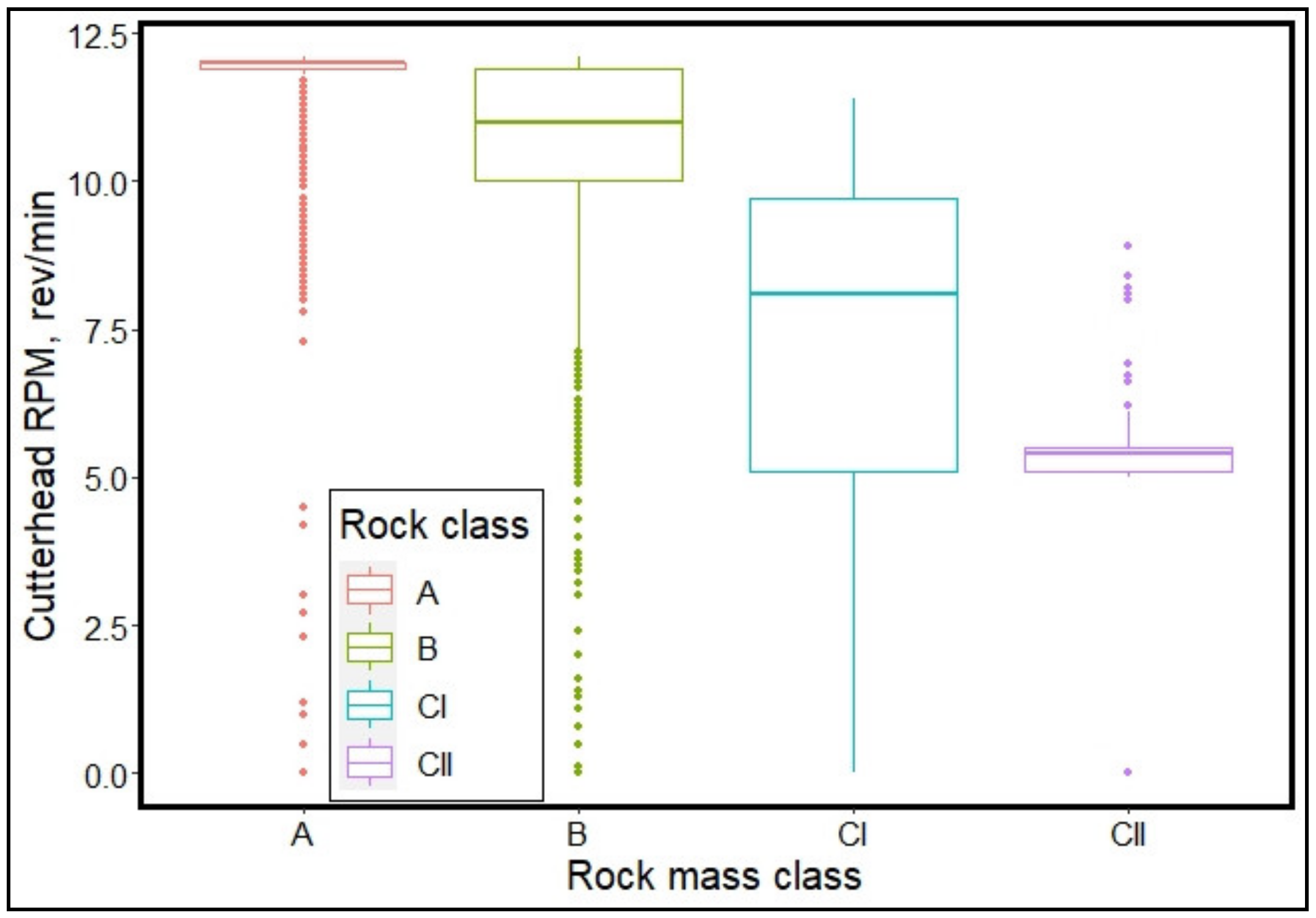
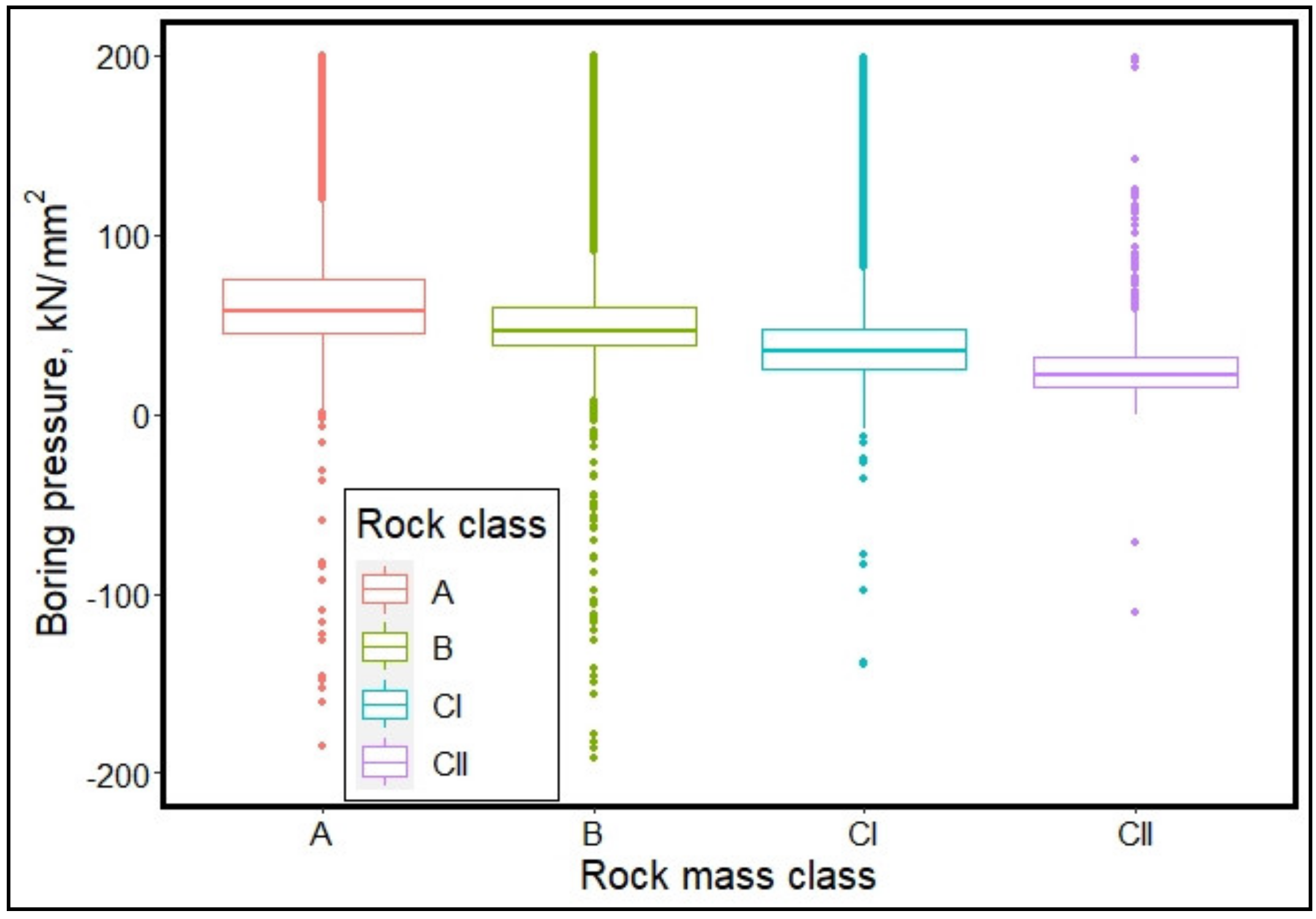
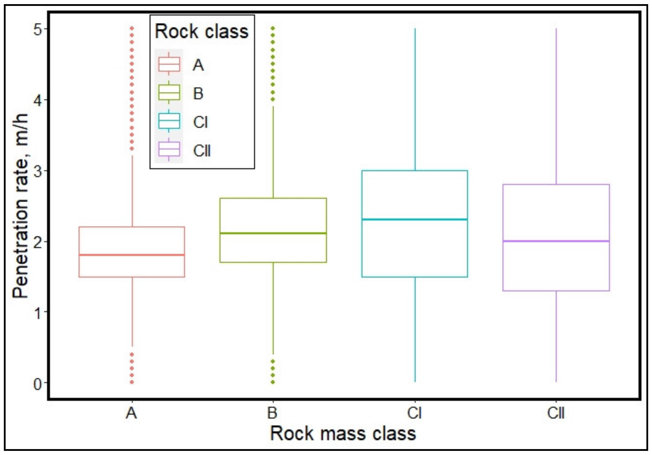
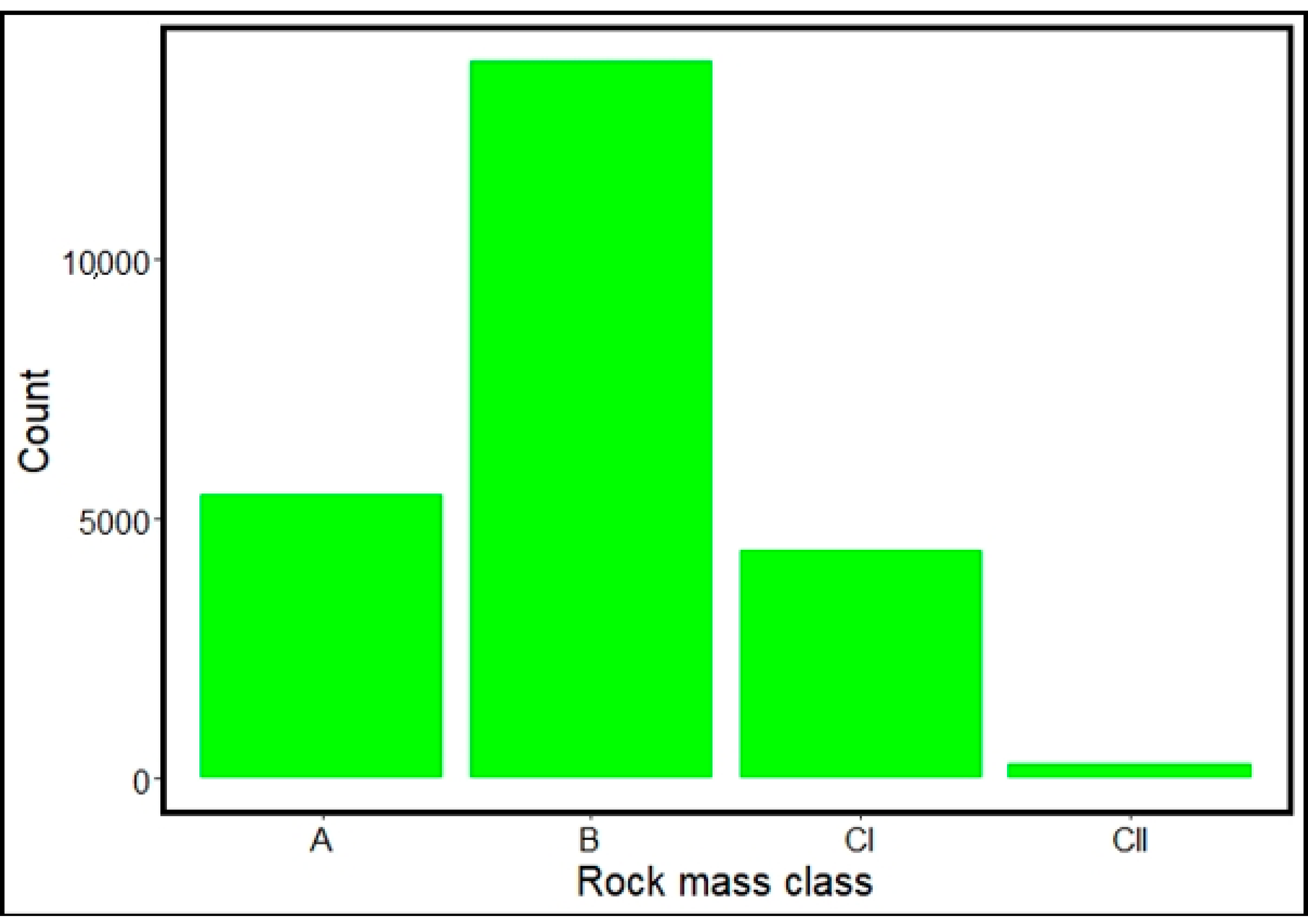
3.1. Data Exploration

The dataset used in this study contained 23,947 records after cleaning to remove missing values, and duplicates. A summary of the input variables is presented in Table 3 with the cutterhead torque having the largest range followed by the boring pressure. A pairwise correlation of the input variables presented in Table 4.
Table 4 shows that, apart from stroke speed and penetration rate, that have a strong positive correlation, the rest of the variables have very weak correlations. This shows that there are no concerns of multicollinearity.
From Figure 5, the median cutterhead RPM decreases with decreasing rock mass competence. In a more competent rock mass, the penetration of the cutting tools into the rock mass is limited by the rock mass strength, therefore, the RPM of the cutterhead is higher than when rock mass is less competent (e.g., CII), where the cutting tool penetrates deeper. This is a possible explanation for the behavior of the cutterhead RPM observed in Figure 5.
A close observation of Figure 6 shows a consistent decline in the median boring pressure from rock class A through rock class CII. This general decline in the applied pressure can be attributed to the decrease in the integrity of the rock mass from class A to CII. Massive competent rock, like rocks in class A, will require high excavation pressure for fragmentation than fractured rock such as those in class CII. In each rock type, the boring pressure is widely variable with a lot of outliers (Figure 6). This variability stems from instantaneous heterogeneities that are encountered within one rock mass class. The variability is more pronounced in the first three classes and not as much in class CII.
In terms of the rate of penetration or advancement rate, the median penetration rate increased from class A to class CI. This is intuitive since it is expected to be more difficult to advance in competent rock. CII however, shows an unexpected low penetration rate as shown in Figure 7. This may be attributed to other operation factors that accompany excavation in relatively weak rocks like class CII.
The dataset had an obvious imbalance in the number of data points in each rock mass class (Figure 8, Table 5). This imbalance tends to affect the performance of classification models. Majority of the rock mass in the dataset were in class B. The number of rock mass data points in classes A and CI are comparable with only a small fraction of the dataset falling in class CII. Due to this imbalance, an oversampling technique was employed to obtain a balanced training dataset for unbiased learning of the ML models. The upSample() function in the caret package in the R software was used to conduct the oversampling of the minority classes, A, CI, and CII to equal the majority class, B. It must be stated that the oversampling was only conducted in the training set and not the test set since an imbalance in the test set does not affect the performance of the already trained models.
As stated in Section 1.1, the Japanese highway classification system has six rock classes, but the dataset used in this study only contained four rock classes, A through CII. These classes fall in the general category of hard rock. Therefore, this study is applicable to hard rock tunnel excavations.

3.2. Variable Importance

A sensitivity analysis was conducted to ascertain the level of influence each input variable has on the models’ classification capabilities. Permutation of each input variable was done while keeping the rest of the input variables constant and the mean decrease in Gini index, a measure of total variance across the rock mass classes, was recorded. The higher the mean decrease in Gini index, the higher the sensitivity to that variable.
Based on this analysis, cutterhead RPM is the most sensitive variable to the rock mass class followed by the cutterhead thrust (Figure 9). Zhang et al. [8] observed a similar relationship between cutterhead torque, cutterhead thrust, and rock mass classes, and concluded that torque and thrust were good indicators of rock mass behavior. The least sensitive variables are the stroke speed and rate of penetration, respectively. The high sensitivity to the cutterhead RPM is somewhat intuitive since it is directly related to the integrity of the rock mass being excavated. With the same level of cutterhead torque, RPM will decrease significantly in less competent rock masses (e.g., class CII) as compared to more competent rock (e.g., class A) as seen in Figure 5. A similar analogy can be given for the cutterhead thrust. In general, it is expected that the rate of excavation/penetration would increase significantly when cutting class CII as compare to operating in class A. This was observed from class A through CI but the rate of penetration decreased in CII. The rate of penetration can be affected by several factors such as intentional maneuvers by the operator due to the unstable nature of the weak rocks (e.g., class CII). This response can be seen in Figure 7.

4. Development of Machine Learning (ML) Models

Two machine learning techniques, random forest, and extremely randomized trees, were applied to develop models for classifying the rock mass dataset into categories based on JH rock classification system. This section discusses the data preprocessing, machine learning models that were applied, and their learning process.

4.1. Data Preprocessing

The TBM operation parameters were recorded at a much higher resolution, about a fraction of a meter, as compared to the rock mass data, which were collected every 4 to10 m. The rock mass data was taken at a coarse resolution because the rock properties in this section of the tunnel were not changing much within a short interval. Where a change in rock mass characteristics was observed, a finer rock mass data collection resolution was used in order to capture all the variations in the rock mass. Another possible reason for coarser resolution in the rock mass data is that taking the rock mass data involves shutting down the operations to allow for geologist to be able to access the tunnel walls. On the other hand, the machine operating parameters are easier to collect and does not require any downtime. For this study, the resolution of the machine data and the rock mass data had to be matched to enable usage of the machine data to predict the rock mass conditions. The chainage interval in the two datasets was used as a key to match the two datasets. That is, the rock mass record for a particular chainage interval is adjoined to all the TBM records in that chainage interval. This was done for all the data points in the rock mass dataset, creating the aggregate dataset used for this study.
The variables in the dataset consist of a wide range of scales, tens to thousand. Consequently, the data was normalized so that the input variables are in the same scale. According to Jayalakshmi and Santhakumaran [26], normalization helps minimize bias caused by different scales of the input variables. Computational speed is also improved by data normalization since the features are put on the same scale. As a result, that dataset in this study was normalized using the min-max normalization which preserves the relationship between the input and output variables. The input variables were scaled to a range between a minimum of zero and a maximum of one. The preProcess() function in R software was used to normalize the data in this study. The normalization is achieved using Equation (1) [26].
x = x m a x x m i n × x i x m i n x m a x x m i n   +   x m i n
where x is the rescaled feature x, x m a x is the maximum value of feature x, x m i n is the minimum value of feature x, and x i is the ith value of feature x.

4.2. ML Models Description

4.2.1. Random Forest (RF)

According to Zhang and Ma [23], random forest (RF) has been applied successfully in a wide variety of projects and has seen tremendous acceptance in many disciplines, thus, its inclusion in this study. RF also has the capability of ranking the importance of all the input variables contributing to the prediction of the target variable.
The predictive abilities of multiple decision trees are harnessed by Random Forest, an ensemble method. To practice each decision tree, bootstrapped samples are used and the predictive capabilities of all the trained trees are aggregated to form the final model. A number of predictors, mtry, was randomly chosen in constructing the trees to be considered at each node during the recursive binary splitting instead of using all the predictors [27]. This gives the technique its name, random forest. At each node, a different set of predictors are used for node splitting; therefore, the variance of the resulting model is significantly reduced compared to the individual regression tree. In training the decision trees, each split is done to obtain two regions R1 and R2 as in Equation (2).
R 1 j ,   s   =   { X | X J   <   s }   a n d   R 2 j ,   s   =   { X | X J     s }
where j is the index in the predictor space with an upper limit of mtry and s is the cut point for the split.
The objective is to obtain j and s values that minimize the function (Equation (3)).
i : x i ϵ R 1 j , s y i y ^ R 1 2 + i : x i ϵ R 2 j , s y i y ^ R 2 2
with y ^ R 1 is the mean response for the training observations in R1(j, s); and y ^ R 2 is the mean response for the training observations in R2(j, s).
This process is repeated until there is no decrease in residual sum of squares by further splitting, at which point the terminal node is reached. The number of predictors to be considered in the splitting at the nodes, mtry, is a hyperparameter that has been calibrated using 5-fold cross-validation (CV) to achieve an optimum value for the best prediction output in training the random forest model [27]. The optimal mtry was then used to fit the final model.

4.2.2. Extremely Randomized Tree (ERT)

ERT is also an ensemble method similar to RF. The difference between RF and ERT is in the mode of tree nodes splitting. While the splitting is deterministic in RF, it is randomized in ERT. The randomized splitting in ERT has the tendency to further reduce the prediction variance when the dataset has a low level of noise. This implies that when the dataset is less noisy, ERT tends to perform significantly better than RF. However, when the data is noisy ERT does not necessarily have an improved performance over RF. Due to the randomized nature of node splitting, ERT is more computationally expensive than RF. Therefore, if the performance of ERT is not significantly better than that of RF, it is recommendable to adopt RF. A detailed description of ERT can be found in [28]. ERT is considered in this study because of its semblance to the RF model which has proven to be effective in predicting mechanical excavator’s performance [29] and its tendency to have improved performance over RF.

4.3. Machine Learning Process

Since the response variable—rock mass class—has four levels, multi-class classification was conducted using Random Forest and Extremely Randomized Trees. The models were trained on 70% of the dataset and the remaining 30% was used to evaluate their classification performance. These fractions were chosen because the dataset is large and oversampling of the minority classes in the training set further increased the size of the training set, hence, 70% of the data was used for the model training instead of the usual 80% that is generally used.
During the model training, 5-fold CV was used to tune the hyperparameters of the models. In RF, the hyperparameter, mtry, is the number of predictors that are considered in deciding the best split at each decision node [27]. The mtry for this dataset was 5. The hyperparameters for the ERT are mtry and numRandomCuts. numRandomCuts is the number of randomly selected splits for each mtry. The mtry and numRandomCuts in this study were both 6. After obtaining the optimal hyperparameters the cross-validation run, the final models were then fitted using these hyperparameters.

4.4. ML Model Performance Metrics

4.4.1. Accuracy and Balanced Accuracy

Accuracy is the measure of correct classifications. It is the ratio of the number of observations that are correctly classified to the total number of observations. This metric is only meaningful when evaluating balanced datasets. It loses its relevance when evaluating an unbalanced dataset [30]. In studies involving unbalance datasets, balanced accuracy is a more meaningful performance metric. It is calculated as the average of the proportion corrects of each class individually, that is, the arithmetic mean of the precision and recall (Equation (4)).
b = p + r e 2
where b is the balance accuracy, p is the precision, and re is the recall

4.4.2. F1 Score

Precision measures the proportion of positive classifications that are correct in binary classification. It is the ratio of the number of correct positive classifications to the total number of positive observations [30]. Recall is a measure of the proportion of actual positives that are identified correctly. This is also known as the sensitivity of the model [30]. There is usually a trade-off between precision and recall depending on the purpose of the classification and the risk associated with the false-positive classification. The F1 score is the harmonic mean of precision and recall (Equation (5)).
F 1 = 2 × p × r e p + r e

4.4.3. Cohen’s Kappa Coefficient (k)

Kappa is a statistical measure of the agreement between different raters [31]. In this case, it is the measure of the agreement between the predicted and observed rock mass classes. Unlike accuracy, kappa takes into account classifications made by chance. It is given by Equation (6). The following descriptions are given to various ranges of kappa: 0 = agreement equivalent to chance; 0.1–0.20 = slight agreement; 0.21–0.40 = fair agreement; 0.41–0.60 = moderate agreement; 0.61–0.80 = substantial agreement; 0.81–0.99 = near perfect agreement; 1 = perfect agreement [31]. In formula,
k = p 0 p e 1 p e
where p 0 is the relative observed agreement among raters; and p e is the hypothetical probability of chance agreement.

5. Results and Discussion

5.1. Classification Performance the ML Models

The overall performance of the ML models was measured by the accuracy and Cohen’s kappa. These were calculated by considering all the correct predictions and all the wrong predictions. The performance of the models in predicting each rock class was measured by the F1-score and balanced accuracy. Since the study involved a multi-class classification, the performance metrics were computed by considering one class, e.g., class A, as positive, while the other three classes, e.g., classes B, CI, and CII, were considered negative. This was done until each rock mass class was considered positive to obtain the metrics presented in Table 6.
Based on the F1-score and the balanced accuracy, both RF and ERT accurately predicted rock class CII with at least 96% in terms of the F1-score and 99% in terms of the balanced accuracy. The worse model performance was recorded when predicting class A with F1-score of at least 92% and balanced accuracies of 95%. The variation in performance level in predicting the different rock mass classes could be related to the TBM operation and excavation process. Rock mass class A consists of slightly weathered with few or no fractures, to fresh massive granites, which causes excessive cutter wear resulting in frequent replacement of consumable components, e.g., cutters. This wear and tear, and subsequent replacement of cutters can cause fluctuations in the TBM operating parameters and could have resulted in the low prediction performance of class A as can be seen Table 6. As the rock mass gets highly weathered and intensively fractured, like rock mass classified as CII, less cutter wear will be observed, resulting in a fairly consistent set of operating parameters, all other factors held constant. This can also be seen in Figure 6, where the boring pressure showed less variability in class CII as compared to the rest of the rock mass categories. In general, more consistent set of operating parameters should lead to models with high prediction performance. In terms of classifying the overall rock mass in the various rock mass classes, both models performed very well with the overall accuracy greater than 0.94 and Cohen’s kappa greater than 0.90, as shown in Table 7.
Visual presentation of the classification by the two models in the form of confusion matrix heatmaps are shown in Figure 10 and Figure 11. The counter-diagonal boxes (top right to the bottom left corner) represent correct prediction of the rock mass class while the rest of the boxes represent misclassification. The intensity of the fill color of the boxes represents the proportion of the data points that have been categorized into that class by the model (misclassification and correct classification). It is interesting to note that in both models, class A was only misclassified as class B but was not CI or CII (Figure 10 and Figure 11). Class B was misclassified as A and CI on a few occasions and only misclassified as CII once. The misclassifications of CI were mostly as B with only one being labeled as class A by RF and three labeled as CII. Both models only misclassified CII as CI once. This shows that the models do not predict rock classes that are far off from the actual class, especially in the case of A and CII. This means that on a very worst-case scenario of misclassification, there is still confidence that the prediction is within the immediate neighborhood of the actual rock mass class. Since the predicted rock mass classes will be used to determine the required support type, it would be detrimental to classify CII as A and assume that it needs no support. On the other hand, classifying A as CII will result in an unnecessary escalation of the project cost in terms of the needed ground support for class CII.

5.2. Comparison of the ML Models

The overall classification performance of the two models was compared using bootstrap sampling. 1000 bootstrap samples were taken from the test dataset with replacement and the performance of both models was tested on each sample set. This gave normal distributions of accuracy and kappa (Figure 12). The mean performance of ERT is higher than that of RF, however, the 95% confidence interval for the two models overlap in terms of both accuracy and kappa as shown in Table 8.
This indicates that statistically, ERT does not significantly outperform RF.

6. Conclusions

In this study, two machine learning (ML) classification algorithms; random forest and extremely randomized trees, were employed to characterize and classify ground conditions along the Pahang-Selangor Raw Water Transfer (PSRWT) tunnel alignment in Malaysia based on TBM operating parameters and rock mass data obtained based on JH rock mass classification system. The TBM operating parameters included in this approach are rate of penetration, cutterhead torque, cutterhead thrust, cutterhead revolution per minute, hydraulic cylinder stroke speed, boring pressure, and motor amps. Due to imbalance in the rock mass data, an oversampling technique was used to obtain a balanced training dataset for unbiased learning of the machine learning (ML) models. Multi-class classification was done, categorizing the rock mass condition into A, B, CI, and CII classes per the JH system. The JH classification system categorizes rock mass into six classes but the tunnel section from which the dataset was obtained consisted primarily of hard rocks. Consequently, only rock classes consistent with hard rock were encountered and analyzed in this paper. An extension of this study is needed with a dataset that includes all the soft rock mass classes to make the developed models compressive in all ground conditions that the TBM may encounter along the tunnel tract.
The main conclusions of this study can be summarized as follows:
  • The proposed approach was applied to a dataset from the Pahang-Selangor Raw Water tunnel (PSRWT) project in Malaysia. A comparison between the ML model classification results and the measured rock mass classes shows that the proposed approach is effective. The identification and classification accuracies were 95% and 94% for ERT and RF, respectively with kappa values of at least 0.90.
  • A bootstrap comparison of the performance of the two ML models, RF and ERT, indicated no model outperformed the other. Due to the randomized nature of node splitting, ERT is more computationally expensive than RF. Therefore, if the performance of ERT is not significantly better than that of RF, it is recommendable to adopt RF.
  • The most influential TBM operating parameter in classifying the rock mass is the cutterhead RPM followed by cutterhead thrust. The two least influential parameters are stroke speed and rate of penetration. Therefore, TBM thrust and RPM can be adjusted in real-time by determining the rock mass class being excavated using the ML models developed in this paper.
  • From a practical standpoint, the overall results obtained in this study show that the data-oriented approach is a useful tool for on-the-fly rock mass conditions identification, characterization and classification of ground conditions along tunnel alignment. It can be a tool for on-site decision making such as selecting support systems or refining preliminary support systems based on ground condition encountered.
  • Extension of this research should also focus on exploring other ML techniques including deep learning methods as well as developing a framework for operationalizing this approach in TBMs.

Author Contributions

Conceptualization, S.S.-N., P.E.A.A. and A.G.A.K.; data curation, S.S.-N. and P.E.A.A.; formal analysis, A.G.A.K., S.S.-N. and P.E.A.A.; methodology, S.S.-N., P.E.A.A. and J.W.A.A.; software, P.E.A.A. and J.W.A.A.; supervision, H.Z. and Z.Z.; writing—original draft, S.S.-N., P.E.A.A. and A.G.A.K.; writing—review & editing, A.G.A.K., F.A. and Z.Z. All authors have read and agreed to the published version of the manuscript.

Funding

This research was funded by the Ministry of Higher Education (MOHE), Malaysia grant number 6071221 And The APC was funded by MOHE.

Acknowledgments

This research was supported by the Ministry of Higher Education (MOHE), Malaysia under the Fundamental Research Grant Scheme (FRGS) of 6071221.

Conflicts of Interest

The authors declare that they have no conflict of interest.

References

  1. Barton, N.; Lien, R.; Lunde, J. Engineering classification of rock masses for the design of tunnel support. Rock Mech. Rock Eng. 1974, 6, 189–236. [Google Scholar] [CrossRef]
  2. Bieniawski, Z.T. Geomechanics classification of rock masses and its application in tunneling. In Proceedings of the 3rd International Congress on Rock Mechanics, Denver, CO, USA, 1 September 1974; p. II-A. [Google Scholar]
  3. Palmstrøm, A. Characterizing rock masses by the RMi for use in practical rock engineering. Tunn. Undergr. Space Technol. 1996, 11, 175–188. [Google Scholar] [CrossRef]
  4. Hoek, E.; Brown, E.T. Practical estimates of rock mass strength. Int. J. Rock Mech. Min. Sci. 1997, 34, 1165–1186. [Google Scholar] [CrossRef]
  5. Jalalifar, H.; Mojedifar, S.; Sahebi, A. Prediction of rock mass rating using fuzzy logic and multi-variable RMR regression model. Int. J. Min. Sci. Technol. 2014, 24, 237–244. [Google Scholar] [CrossRef]
  6. Shi, S.-S.; Li, S.-C.; Li, L.-P.; Zhou, Z.-Q.; Wang, J. Advance optimized classification and application of surrounding rock based on fuzzy analytic hierarchy process and Tunnel Seismic Prediction. Autom. Constr. 2014, 37, 217–222. [Google Scholar] [CrossRef]
  7. Lee, K.H.; Park, J.H.; Park, J.; Lee, I.M.; Lee, S.W. Electrical resistivity tomography survey for prediction of anomaly inmechanized tunneling. Geomech. Eng. 2019, 19, 93–104. [Google Scholar]
  8. Zhang, Q.; Liu, Z.; Tan, J. Prediction of geological conditions for a tunnel boring machine using big operational data. Autom. Constr. 2019, 100, 73–83. [Google Scholar] [CrossRef]
  9. Liu, Q.; Wang, X.; Huang, X.; Yin, X. Prediction model of rock mass class using classification and regression tree integrated AdaBoost algorithm based on TBM driving data. Tunn. Undergr. Space Technol. 2020, 106, 103595. [Google Scholar] [CrossRef]
  10. Shahriar, K.; Sargheini, J.; Hedayatzadeh, M.; Hamidi, J.K. Performance Prediction of Hard Rock TBM Using Rock Mass Classification. In Rock Mechanics in Civil and Environmental Engineering—Proceedings of the European Rock Mechanics Symposium EUROCK; Taylor & Francis Group: London, UK, 2010; ISBN 978-0-415-58654-2. [Google Scholar]
  11. Mahdevari, S.; Torabi, S.R. Prediction of tunnel convergence using Artificial Neural Networks. Tunn. Undergr. Space Technol. 2012, 28, 218–228. [Google Scholar] [CrossRef]
  12. Mahdevari, S.; Torabi, S.R.; Monjezi, M. Application of artificial intelligence algorithms in predicting tunnel convergence to avoid TBM jamming phenomenon. Int. J. Rock Mech. Min. Sci. 2012, 55, 33–44. [Google Scholar] [CrossRef]
  13. Mahdevari, S.; Shahriar, K.; Yagiz, S.; Shirazi, M.A. A support vector regression model for predicting tunnel boring machine penetration rates. Int. J. Rock Mech. Min. Sci. 2014, 72, 214–229. [Google Scholar] [CrossRef]
  14. Ren, Q.; Wang, G.; Li, M.; Han, S. Prediction of Rock Compressive Strength Using Machine Learning Algorithms Based on Spectrum Analysis of Geological Hammer. Geotech. Geol. Eng. 2018, 37, 475–489. [Google Scholar] [CrossRef]
  15. Xu, H.; Zhou, J.; Asteris, P.G.; Armaghani, D.J.; Tahir, M.M. Supervised Machine Learning Techniques to the Prediction of Tunnel Boring Machine Penetration Rate. Appl. Sci. 2019, 9, 3715. [Google Scholar] [CrossRef] [Green Version]
  16. Zhang, Q.; Hu, W.; Liu, Z.; Tan, J. TBM performance prediction with Bayesian optimization and automated machine learning. Tunn. Undergr. Space Technol. 2020, 103, 103493. [Google Scholar] [CrossRef]
  17. Salimi, A.; Rostami, J.; Moormann, C. Application of rock mass classification systems for performance estimation of rock TBMs using regression tree and artificial intelligence algorithms. Tunn. Undergr. Space Technol. 2019, 92, 103046. [Google Scholar] [CrossRef]
  18. Liu, B.; Wang, R.; Zhao, G.; Guo, X.; Wang, Y.; Li, J.; Wang, S. Prediction of rock mass parameters in the TBM tunnel based on BP neural network integrated simulated annealing algorithm. Tunn. Undergr. Space Technol. 2020, 95, 103103. [Google Scholar] [CrossRef]
  19. Liu, K.; Liu, B.; Fang, Y. An intelligent model based on statistical learning theory for engineering rock mass classification. Bull. Int. Assoc. Eng. Geol. 2018, 78, 4533–4548. [Google Scholar] [CrossRef]
  20. Jung, J.-H.; Chung, H.; Kwon, Y.-S.; Lee, I.-M. An ANN to Predict Ground Condition ahead of Tunnel Face using TBM Operational Data. KSCE J. Civ. Eng. 2019, 23, 3200–3206. [Google Scholar] [CrossRef]
  21. Zhang, Q.; Yang, K.; Wang, L.; Zhou, S. Geological Type Recognition by Machine Learning on In-Situ Data of EPB Tunnel Boring Machines. Math. Probl. Eng. 2020, 2020, 1–10. [Google Scholar] [CrossRef]
  22. Erharter, G.H.; Marcher, T. MSAC: Towards data driven system behavior classification for TBM tunneling. Tunn. Undergr. Space Technol. 2020, 103, 103466. [Google Scholar] [CrossRef]
  23. Zhang, C.; Ma, Y. Ensemble Machine Learning: Methods and Applications; Springer: Berlin, Germany, 2012. [Google Scholar]
  24. Shinji, M.; Akagi, W.; Shiroma, H.; Yamada, A.; Nakagawa, K. JH Method of Rock Mass Classification for Tunnelling. In ISRM International Symposium - EUROCK 2002, 25-27 November, Madeira, Portugal; International Society for Rock Mechanics and Rock Engineering: Lisbon, Portugal, 2002; pp. 375–383. [Google Scholar]
  25. Abad, S.A.N.K.; Mohamad, E.; Komoo, I. Dominant weathering profiles of granite in southern Peninsular Malaysia. Eng. Geol. 2014, 183, 208–215. [Google Scholar] [CrossRef]
  26. Jayalakshmi, T.; Santhakumaran, A. Statistical Normalization and Back Propagationfor Classification. Int. J. Comput. Theory Eng. 2011, 89–93. [Google Scholar] [CrossRef]
  27. James, G.; Witten, D.; Hastie, T.; Tibishirani, R. An Introduction to Statistical Learning with Applications in R (Older Version); Springer US: New York, NY, USA, 2013. [Google Scholar]
  28. Geurts, P.; Ernst, D.; Wehenkel, L. Extremely randomized trees. Mach. Learn. 2006, 63, 3–42. [Google Scholar] [CrossRef] [Green Version]
  29. Seker, S.E.; Ocak, I. Performance prediction of roadheaders using ensemble machine learning techniques. Neural Comput. Appl. 2019, 31, 1103–1116. [Google Scholar] [CrossRef]
  30. Fürnkranz, J.; Chan, P.K.; Craw, S.; Sammut, C.; Uther, W.; Ratnaparkhi, A.; Jin, X.; Han, J.; Yang, Y.; Morik, K.; et al. Mean Absolute Error. In Encyclopedia of Machine Learning; Springer Science and Business Media LLC: Berlin, Germany, 2011; p. 652. [Google Scholar]
  31. Glen, S. Cohen’s Kappa Statistic. Statistics How To. 2014. Available online: https://www.statisticshowto.com/cohens-kappa-statistic/ (accessed on 4 November 2020).
Figure 1. Robbins 5.2 m diameter main beam Tunnel Boring Machine (TBM).
Applsci 11 01060 g001
Figure 2. Geologic map of the study area.
Applsci 11 01060 g002
Figure 3. Schematic cross section of the tunnel alignment.
Applsci 11 01060 g003
Figure 4. Tunnel zones during characterizations.
Applsci 11 01060 g004
Figure 5. Distribution of cutterhead RPM in different rock mass classes.
Applsci 11 01060 g005
Figure 6. Distribution of boring pressure in different rock mass classes.
Applsci 11 01060 g006
Figure 7. Distribution of TBM penetration rate in different rock mass classes.
Applsci 11 01060 g007
Figure 8. Amount of data from each rock class showing an imbalanced dataset.
Applsci 11 01060 g008
Figure 9. Sensitivity level of rock mass class to input variables based on mean decrease in Gini index expressed a percentage of the maximum Gini index.
Applsci 11 01060 g009
Figure 10. Confusion matrix of the classification performance of the RF model.
Applsci 11 01060 g010
Figure 11. Confusion matrix of the classification performance of the ERT model.
Applsci 11 01060 g011
Figure 12. Distribution of kappa and overall accuracy of the ML models obtained from a bootstrap sampling of the test.
Applsci 11 01060 g012
Table 1. Example of the JH System Data Collection Sheet Used in the PSRWT project.
Geological ObservationRating
1. Strength of the intact rock materialUniaxial Comp. strength.>100 MPa100–50 MPa50–25 MPa25–10 MPa10–3 MPa<3 MPa
Point-load Strength.>3 MPa4–2 MPa2–1 MPa1–0.4 MPa<0.4 MPa--
Strength judged by blow of hammerNot broken by strong blow of hammerBroken by strong blow of hammerBroken by normal blow of hammerBroken by striking rocks against each otherBroken easily by handDeformed by finger
Grade Point3629221470
2. Weathering/AlterationDegree of weatheringFreshWeathered along discontinuitiesWeathered to the rock mass coreSedimentary Unconsolidated
Hydrothermal alterationNo AlterationPartially altered and infilled with clayAltered and weakened to the rock coreheavily altered and become clayey or sedimentary
Grade Point191260
3. Spacing of discontinuities, mmSpacing of Discontinuity.D = 1 m1 m > d = 50 cm50 > d = 20 cm20 > d = 5 cm5 cm > d
R.Q.D>8080–5060–3040–10<20
Grade Point1914950
4. Condition of discontinuitiesDegree of openingFracture Totally-attachedFracture Partly openedFracture mostly openedFracture opened
–5 mm width
Fracture opened
>5 mm
Infilled widthNilNilNilClay(<5mm)Clay (>5mm)
Degree of RoughnessCoarseFlat and SmoothPartly SlickensideWell-sharpened slickenside
Grade Point26201370
5. Effect of discontinuity strike and dip orientation declinationStrike perpendicular to Tunnel Axis1. Drive with dip-Dip 45–902. Drive with dip-Dip 20–453. Drive with/against dip-Dip 0–204. Drive against dip-Dip 20–454. Drive against dip-Dip 45–90
EvaluationVery favorableFavorableNormalUnfavorableFair
Strike parallel to Tunnel Axis----1. Dip 0–202. Dip 20–453. Dip 45–90
Evaluation----NormalUnfavorableFair
Evaluation on Ground water and Degradation (including the possibility in the future) at the length of 10 m from face
6. GroundwaterAmount of inflow per 10m tunnel length<1 L/min1–20 L/min20–100 L/min>100 L/min
General conditionsDry/MoistWetDripping waterFlowing water
Classification1234
7. Degradation by waterDegradation by waterNilPartially weakenedLoosenedWashed out
Classification1234
Table 2. Rock Mass Classes and Support Requirement of JH System (modified after Shinji et al. [24]).
Rock ClassRange of Total Grade Points (%)DescriptionSupport Requirement
A100–90Very good rock, hard and freshNo support
B89–70Good rock, hard and fresh but affected by weatheringSpot bolting, shotcrete to crown/wall
CI69–51Fair rock, rock is weathered, some clay in jointsPattern bolting to crown, shotcrete to crown/wall
CII50–40Fair to poor rock weathered, loosed rock massPattern bolting to crown/wall, shotcrete to crown/wall
D39–20Very poor to extremely poor rocks: considerably weathered rock mass, soft zones, partially soil propertiesPattern bolting to crown/wall, shotcrete to crown/wall, steel rib
E<20Faults and crushed rock zone, squeezing zonesPattern bolting to crown/wall, shotcrete to crown/wall, steel rib, steel lagging
Table 3. Summary statistics of the TBM data.
TBM ParameterMeanMedianMinimumMaximum
Boring pressure (N/mm2)56.3547.10−5448.201155.80
Cutterhead torque (kN-m)562.57622.00−31,96222,523.00
Cutterhead thrust force (kN)9910.1510,619.000.0011,424.00
Cutterhead RPM (rev/min)10.2911.000.0012.10
Rate of penetration (m/h)2.302.100.00107.80
Stroke speed (mm/min)38.1835.000.001797.00
Gripper cylinder pressure (bar)301.67306.000.00691.00
Pitching (°)−0.06−0.09−0.521.26
Average motor amps (A)138.79138.000.00427.00
Table 4. Pairwise correlation of some input variables.
TBM ParameterBoring PressureCutterhead TorqueCutterhead Thrust ForceCutterhead RPMRate of PenetrationStroke SpeedGripper Cylinder PressurePitchingAverage Motor Amps
Boring Pressure1.00
Cutterhead torque0.211.00
Cutterhead thrust force0.260.281.00
Cutterhead RPM0.14−0.030.451.00
Rate of Penetration−0.100.050.07−0.021.00
Stroke speed−0.100.050.07−0.010.981.00
Gripper Cylinder pressure0.070.080.380.400.090.071.00
Pitching0.04−0.04−0.060.140.00−0.01−0.091.00
Average motor amps0.110.230.41−0.070.210.220.24−0.021.00
Table 5. Amount of data from each rock class before and after oversampling the minority classes.
Rock ClassCount
UnbalancedBalanced
A546013,817
B13,81713,817
CI438213,817
CII28813,817
Table 6. Performance metrics of the ML models in predicting each rock class.
Random ForestExtremely Randomized Trees
Rock ClassF1 ScoreBalanced AccuracyF1 ScoreBalanced Accuracy
Class: A0.920.950.930.95
Class: B0.950.940.960.95
Class: CI0.950.970.960.97
Class: CII0.960.990.970.99
Table 7. Overall performance metrics of the ML models.
ModelAccuracyKappa
Random forest0.9420.901
Extremely randomized trees0.9500.914
Table 8. 95% confidence intervals of the overall performance metrics of the ML models.
ModelMetricLower (2.5%)50.0%Upper (97.5%)
Random forestKappa0.8890.9010.912
Extremely randomized trees0.9020.9130.924
Random forestAccuracy0.9350.9420.949
Extremely randomized trees0.9440.9500.956
Publisher’s Note: MDPI stays neutral with regard to jurisdictional claims in published maps and institutional affiliations.

