Ambulance Locations in a Tiered Emergency Medical System in a City

Abstract

This paper deals with optimizing the location of ambulance stations in a two-tiered emergency medical system in an urban environment. Several variants of station distribution are calculated by different mathematical programming models and are evaluated by a detailed computer simulation model. A new modification of the modular capacitated location model is proposed. Two ways of demand modelling are applied; namely, the aggregation of the ambient population and the aggregation of permanent residents at the street level. A case study of the city of Prešov, Slovakia is used to assess the models. The performance of the current and proposed sets of locations is evaluated using real historical data on ambulance trips. Computer simulation demonstrates that the modular capacitated location model, with the ambient population demand, significantly reduces the average response time to high-priority patients (by 79 s in the city and 62 s in the district) and increases the percentage of high-priority calls responded to within 8 min (by almost 4% in the city and 5% in the district). Our findings show that a significant improvement in the availability of the service can be achieved when ambulances are not accumulated at a few stations but rather spread over the city territory.

1. Introduction

Emergency medical services (EMS) play the main role in pre-hospital medical care. Their goal is to provide timely and appropriate treatment to patients with emergency medical conditions and transport them to the nearest appropriate healthcare facility. Patients’ survivability and morbidity are affected by the efficiency of the interventions that, in turn, depend on the ambulance base location, the ambulance allocation to the stations, and ambulance dispatching decisions. Planning EMS at all levels (strategic, tactical, and operational) represents a challenging problem that is still topical in the constantly changing socioeconomic environment.

The ambulance location is an optimization problem that deals with the location of the base stations where the vehicles providing emergency medical services are housed. The problem has attracted researchers’ attention for more than 40 years. Several excellent review papers trace the evolution of modelling approaches [1,2,3]. The importance of sitting emergency facilities has not diminished over the years because population ageing leads to a growing demand for healthcare, including urgent pre-hospital care [4,5]. In addition, the increasing availability of demographic, geographical, and transportation data allows for designing better optimization location models [6]. Incorporating more detail makes the models more exact and enables them to better reflect the real operation of the system. Simultaneously, mathematical programming solvers such as CPLEX and Gurobi are constantly being improved, and they are becoming more able to solve more complicated models, e.g., [7].

This paper deals with tactical decisions about locating EMS stations in an urban area. We are trying to improve the existing EMS system. We respect the current number of stations but look to locate them in a better way, with the view to increase the availability of the service, especially for patients in critical conditions. We concentrate on the main goal of EMS—to provide a rapid response to medical emergencies. The costs associated with the opening of stations, or the costs of relocating them from their current positions, are not considered because it is beyond the scope of our research to look for potential locations where the stations can be sited and thus to estimate investment costs related to the candidate locations. Instead of considering the costs associated with every closed or open station, one can limit the number of stations that can be relocated under a given budget constraint. Currently, we suppose that no stations can be added, but there are no limitations regarding the number of relocated stations. In general, the costs of constructing EMS stations are hard to predict, so most studies omit them and focus on performance criteria. If the costs are taken into account (e.g., [7,8]), then they are determined empirically without serious justification.

The growing availability of demographic data and data on road networks enables us to better predict where people demanding EMS are located. Two principal approaches have been applied so far to model demand zones in a city. Either the city needs to be covered by a rectangular grid [9,10,11,12,13], with a grid element that corresponds to a demand zone; or, the demand zones need to be identified with urban administrative units, such as census areas [14], city zones [15], postal codes [6], and suburbs [16]. The modelling approach depends on the data availability. The studies using a grid structure usually identify the demand for EMS with historical calls archived by an information system. On the other hand, when demand zones correspond to census areas or other territorial units, then the demand usually corresponds to the population of the unit. This latter method allows for the incorporation of demographic characteristics, such as gender or age, into the demand prediction [14]. However, we are not aware of a comparative study that would recommend one or the other method. That is why we decided to use both methods in our research and assess them by means of computer simulation. For the grid model, we have used the LandScan data model that contains the average number of people over 24 h in cells of approximately 1 km². Instead of large census units, we investigate a more detailed demand model. We draw inspiration from the local administration of the city of Prešov (https://egov.presov.sk/, accessed on 18 December 2021) that publishes and updates, weekly, the number of citizens in every street in the town. A benefit of having such data is that every street may be regarded as a separate demand zone and the center of the street as an aggregated demand point. Such a microscopic approach enables the EMS system to reflect the urban development and to relocate resources closer to residents.

The number of articles related to EMS planning has grown rapidly during the last two decades. This growth may be attributed to increases in the availability of data and in the power of decision-supporting software tools. Several survey articles have been published during this period. A recent survey of location models applied to healthcare facilities was presented by Ahmadi-Javid et al. [2]. The authors focused on the two most frequent types of problems, namely, the covering and median problems. The former class of problems uses the concept of coverage as an analogy to a typical performance measure of an EMS system, such as the proportion of patients responded to within a certain time standard [17,18]. If a patient is reached by an ambulance within the time limit, they are said to be covered by the service. The goal is either to cover the whole region with a minimum number of facilities, or to maximize the number of customers covered by a fixed number of facilities. In the latter group of problems, the so-called median problems, the quality of service is identified with the travel time that patients take to get to the closest facility, or the response time that ambulances need to reach the patients. Both types of problems admit several variations to allow for additional criteria and constraints from real-world applications.

Optimization problems related to the emergency medical services are surveyed in [19]. Aringhieri et al. draws readers’ attention to the shortcomings of various models for location of emergency centers. They point out that coverage or time-based performance measures are only a proxy for health outcomes. The drawback of the coverage concept is that it distinguishes only two states of a patient, covered or not covered. The response time does not play a role if it is below the time limit. Therefore, the same level of service is said to be provided if an ambulance comes in 1 min or in 15 min (in the event of a 15-min standard). In addition, patients who are not covered do not contribute to the objective function value at all, so their response times may be arbitrarily long.

Another shortcoming of the former coverage models, such as the location set covering problem or the maximal covering location problem, is that they are based on a simplifying assumption that ambulances are always available when they are needed. The result is that the solution overestimates the real coverage. The maximum expected covering location problem (MEXCLP) offers a more realistic way of modelling the ambulance availability. It aims to locate a given number of ambulance stations in order to maximize the expected coverage, which depends on the busy fraction, defined as the probability that an ambulance is unavailable to immediately respond to an emergency call. The MEXCLP has been widely reported in the context of the EMS design. It is recommended by Erkut et al. [20] to be applied instead of the maximum availability/reliability models that also deal with the uncertain availability of ambulances but lead to a design that is too expensive. A modified MEXCLP model was used to optimize the distribution of ambulances in Edmonton, Canada [21]. Ingolfsson et al. considered the variation in pre-trip preparation and travel times, and included correction factors that accounted for the dependence in the busy fractions between ambulances. Stochastic response times were also used in [22]. The uncertainty is expressed as a probability that the demand point, j, will be reached by an ambulance from the base, i, within the time threshold. Van den Berg et al. demonstrated their approach in the region of Amsterdam, Netherlands. The study [9] enhanced the MEXCLP by considering multiple customer types, as well as two different types of emergency vehicles. The objective was to maximize the total number of expected Priority 1 calls covered within a specified amount of time. Dispatching rules were included in the model. The experiments were conducted using real-world data collected from Hanover County, Virginia. Sorensen and Church [23] proposed a hybrid model that combined the maximum expected coverage goal of the MEXCLP with the reliability of the service at every demand node. Although the authors reported the superiority of their model compared to the original MEXCLP model, the benefit of the model in practice has not been proved sufficiently, since the results were based on a rather small case study (55 demand nodes) and a simple simulation model. Van den Berg and van Essen [6] assessed several ambulance location models in the view of the performance indicators frequently used in practice. Simulation experiments with real-world case studies showed that the MEXCLP and the expected response time model (ERTM) performed the best. However, the ERTM model is rather complicated, and it takes a long computing time. That is why the average response time model is recommended as a good alternative.

The average response time model is an application-related name for the model of the well-known p-median problem (pMP) that seeks the location of p facilities, so that the average travel time between customers and their closest facility is as short as possible. Several other studies proved the practical applicability of the pMP. For example, Sasaki et al. [14] proposed optimal locations for ambulances in the city of Niigata, Japan. Dzator and Dzator [16] achieved a significant improvement in the average response time by using the pMP for two sub-regions of the Perth Metropolitan area. The pMP was also used in a study by Garner and van den Berg [24] to locate the helicopter emergency medical service bases in the state of New South Wales, Australia.

The weak point of the cited models is the way of modelling ambulance availability. The models either ignore the fact that the closest ambulance may not be idle when it is needed, or they assume that all ambulances are unavailable for the same amount of time. Both these assumptions lead to an oversimplified model.

Hammami and Jebali [7] increased the accuracy of the location model by explicitly considering the ambulance trip time that included not only the response time, but also the on-scene time, the time of transportation to the hospital, the drop-off time, and the travel time from the hospital to the station. Their modular capacitated location model decides on the locations of the stations, the number of ambulances to be assigned to each of them, and the demand allocation to the stations. The objective function is the total system costs, including the station-opening costs, the costs of allocating ambulances to the existing stations, and the transportation costs. This model inspired us, but we had to adapt it to the Franco-German style of EMS delivery that is common in European countries. Hammami and Jebali’s model reflects the Anglo-American system, where all patients are rapidly transported to the hospital with fewer pre-hospital interventions. On the other hand, emergency teams in the Franco-German model are qualified to treat patients in their homes or at the scene. This results in many EMS users being treated at the site of an incident and being transported to hospitals less frequently.

Only few of the mentioned publications compared several location models mutually. If they did, they provided only analytical results that suffered from the same simplifying assumptions that were used in the modelling phase. The only exception is the study by van den Berg and van Essen [6] who use computer simulation to assess the models in realistic situations.

In regard to the solution methods, most ambulance location problems are modelled as mathematical programming problems and are solved by a general-purpose optimization solver [2]. Only a few studies propose such complicated models that cannot be solved to optimality, and require using a metaheuristic method, such as the tabu search [11], variable neighborhood search [10], or ant colony optimization [25].

In this study we propose a modification of the modular capacitated location model [26] and compare it to the most successful models reported in [6,14,16,20,24]; namely, the p-median model, the maximum expected coverage model, and the expected response time model. Firstly, we will evaluate the solutions of the models using the criteria that correspond to their objective functions, namely, the average response time, the expected response time, and the expected coverage within two time thresholds. However, this evaluation is not significant because every model beats the others on its objective function. To assess the models in more realistic settings, we will conduct a simulation study that captures the stochastic character of the system. Computer simulation allows for the estimation of a lot of performance indicators. The most important indicators from the emergency management viewpoint are the average response time, the coverage of high-priority patients, and the coverage of all patients regardless of their priority.

The evaluation of the location models will be done for two different demand models, where the aim will be to reveal whether the demand model has an impact on ambulance location. The first demand model represents the ambient population (an average over 24 h) distribution, and the second one is based only on demographic data on permanent residents aggregated at the street level.

The goal of our study is to answer the following questions:

• Which location model results in the best expected performance in practice?
• Which demand model gives better ambulance deployment?

2. Materials and Methods

We will start this section by the description of the pMP, MEXCLP, and ERTM models. All of them are discrete location models [27]. This means that facilities can be located at the selected potential locations only. In practice, an analyst is supposed to select appropriate candidate locations prior to the optimization.

We introduced a unified notation. The following sets, indices, and parameters are common to all models.

Sets and indices

• I    set of candidate locations
• J    set of demand points
• i ∈ I    candidate location
• i ∈ J    demand point
• $N_j= \left\{i\in I:t_{ij}\le T^{max}\right\}$    set of candidate locations in the neighbourhood of demand point j

Parameters

• p    number of ambulances to be sited
• q    probability of an ambulance being unavailable
• $T^{max}$    the desired service standard (min)
• b_j    weight of demand point j (number of potential patients)
• t_ij    shortest travel time of an ambulance driving at all possible speeds from location i to demand point j (min)

Decision variables

• x_i    the number of ambulances to be located at site i

Except for the location variables, x_i, each of the following models needed additional variables to define its specific objective function.

2.1. The p-Median Problem

To calculate the average travel time between stations and demand zones, the pMP uses the allocation variables z_ij. Variable z_ij is one if the open station at site i is the closest station to demand point j. The mathematical programming model is as follows:

$$minimize {{\displaystyle \sum }}_{i\in I}{{\displaystyle \sum }}_{j\in J}{t}_{ij}{b}_j{z}_{ij}$$

(1)

$$subject to {{\displaystyle \sum }}_{i\in I}{z}_{ij}=1 for j \in J$$

(2)

$$z_{ij}\le x_i for i \in I, j \in J$$

(3)

$${\displaystyle \sum }_{i\in I}{x}_i=p$$

(4)

$$x_i\in \left\{0,1\right\} for i \in I$$

(5)

$$z_{ij}\in \left\{0,1\right\} for i \in I, j \in J$$

(6)

The objective function (1) minimizes the travel time between stations and demand points weighted by demand volume b_j. This criterion reflects the main objective of the EMS system: to provide pre-hospital care as soon as possible. The total travel time can be divided by the total volume of demand to give an average travel time. Constraints (2) ensure that every demand point j lies in the service area of exactly one station. Constraints (3) say that if no station is open at candidate location i, then no demand point j can be served from the location i. Constraint (4) defines the total number of stations in the town. Since placing multiple stations at the same location i would not improve the objective function value, variables x_i are defined as binary by constraints (5). Constraints (6) are the integrality constraints for allocation variables.

2.2. The Maximum Expected Covering Location Problem

The MEXCLP maximizes the number of patients that are likely to have received the service within a given time threshold. We need to know the number of ambulances located in the neighborhood at a demand point. This can be modelled by binary variables, y_jk, that take the value 1 if demand point j is covered by at least k stations. First, we present the formulation of the MEXCLP by Church and Murray [28] that allows a single facility to be placed at a candidate location:

$$minimize {{\displaystyle \sum }}_{j\in J}{{\displaystyle \sum }}_{k=1}^p{b}_j\left(1-q\right)q^{k-1}{y}_{jk}$$

(7)

$$subject to {{\displaystyle \sum }}_{i\in N_j}{x}_i\ge {{\displaystyle \sum }}_{k=1}^p{y}_{jk} for j \in J$$

(8)

$${\displaystyle \sum }_{i\in I}{x}_i=p$$

(9)

$$x_i\in \left\{0,1\right\} for i \in I$$

(10)

$$y_{jk}\in \left\{0,1\right\} for j \in J, k=1, \dots , p$$

(11)

The objective function (7) maximizes the expected coverage of all the demand points, taking into account the possible unavailability of ambulances. For demand point j, the term $b_j\left(1-q\right)q^{k-1}$ represents the increase in the expected coverage brought about by the kth ambulance. According to constraints (8), sitting multiple stations in the neighborhood of demand point j enables multiple variables y_jk to take the value 1 and account for the increase in coverage in the objective function. Constraint (9) limits the number of the located stations. Constraints (10) and (11) impose binary integer restrictions on the decision variables.

In a different version of the model by Marianov and Serra [27], location variables x_i can take non-negative integer values, meaning that multiple ambulances can be allocated to an open station i.

2.3. The Expected Response Time Model

The ERTM minimizes the demand-weighted expected response time [6]. This can be calculated using decision variables, w_ijk, that specify the nearest ambulance, the second nearest ambulance, etc. at every demand point. Variable w_ijk is one if an ambulance located at station i is the kth nearest ambulance to demand point j. The model is as follows:

$$minimize {{\displaystyle \sum }}_{i\in I}{{\displaystyle \sum }}_{j\in J}{{\displaystyle \sum }}_{k=1}^{p-1}{b}_j{t}_{ij}\left(1-q\right)q^{k-1}{w}_{ijk}+{{\displaystyle \sum }}_{i\in I}{{\displaystyle \sum }}_{j\in J}{b}_j{t}_{ij}{q}^{p-1}{w}_{ijp}$$

(12)

$$subject to {{\displaystyle \sum }}_{i\in I}{w}_{ijk}=1 for j \in J, k=1, \dots , p$$

(13)

$$x_i\ge {{\displaystyle \sum }}_{k=1}^p{w}_{ijk} for i \in I, j\in J$$

(14)

$${\displaystyle \sum }_{i\in I}{x}_i=p$$

(15)

$$x_i\in Z^{+} for i \in I$$

(16)

$$w_{ijk}\in \left\{0,1\right\} for i \in I, j \in J, k=1, \dots , p$$

(17)

The first term in the objective function (12) is similar to the expected coverage (7). The second term is the probability that demand points will be served by the farthest (i.e., pth nearest) ambulance. According to constraints (13), every demand point must be served by exactly one ambulance, so the probabilities of being served by the first, second, etc. to pth nearest ambulance must sum up to one. That is why the probability of using the farthest ambulance is $1-{{\displaystyle \sum }}_{k=1}^{p-1}\left(1-q\right)q^{k-1}=q^{p-1}$. Ambulances from a candidate location i may be dispatched to serve demand point j only if at least one ambulance is located at i (14). The remaining constraints were already explained above.

2.4. The Modular Capacitated Location Problem

In this section we propose a modification of the modular capacitated location problem (MCLP). This location problem arose in healthcare strategic planning [26]. Many healthcare facilities may be built from modules of a certain size. The number of patients a facility can serve, as well as the capital and operating costs, depend on the facility size. The size of a facility must be chosen only from a finite and discrete set of possible capacities. Each aggregated customer (a zone or community) can be partially served by more than one facility. A variant of the MCLP for ambulance locations was presented in [7]. Both formulations [7,26] minimize the total costs, consisting of the capital and operating costs of the facilities, as well as the costs induced by serving customers. In this paper we present an adjusted model of the MCLP, where the objective is the average response time to patients. Instead of the costs of opening and operating the facilities, the number of ambulances is limited directly by a given amount. In contrast to the models presented above, this model allows for differentiating patients’ priorities and the service levels provided by the different rescue units. The capacity of an ambulance is expressed as the amount of time when the ambulance is ready for rescue trips. Every trip consumes a portion of this capacity. To model the trip time more precisely, we take into account not only the travel time to the site of the incident, but also the transport to a hospital, the drop-off time at the hospital, and the return to the base station. That is why additional sets and parameters must be introduced.

According to practices in Slovakia and in many other countries, we will distinguish two patient priorities and two levels of EMS. The highest priority is assigned to patients who are in a life-threatening condition. The most severe patient diagnoses include cardiac arrest, stroke, severe respiratory difficulties, chest pain, severe trauma, and unconsciousness. These diagnoses are denoted as the First Hour Quintet (FHQ) because the first hour after a medical incident decides whether the patient survives. An advanced life support (ALS) ambulance is always dispatched when a call-taker at dispatch center assesses the emergency as critical. Non-critical calls may be responded to by a basic life support (BLS) ambulance.

Our model also takes into account a reduced availability of ambulances caused by technical breaks and secondary transports. The secondary transport is a planned activity where an ambulance does not respond to an emergency call but transports patients or medical materials between two healthcare facilities.

In addition to the symbols introduced at the beginning of this section, the following notations will be used in the MCLP model:

Indices

• h    hospital
• k    ambulance type (k = 1—ALS, k = 2—BLS)
• l    patient priority (l = 1—FHQ, l = 2—others)

Parameters

• α_k    the proportion of the interventions of the type k ambulances, which include the transportation of patients to a hospital
• β_k    a correction factor that reduces the availability of the type k ambulances by the time they are occupied with secondary trips and technical breaks
• γ_kl    coefficient; γ_kl = 1 if a type k ambulance can serve the priority l patients and γ_kl = 0 otherwise
• p_k    the maximum number of the type k ambulances
• b_jl    the yearly demand of the priority l patients in demand zone j (the number of patients)
• td    the average drop-off time at the hospital (min)
• ts_kl    the average on-scene time of a type k ambulance serving a priority l patient (min)
• ${\overline{t}}_{ij}$    the travel time of an ambulance driving at a normal speed from location i to its base station j (min)

Since this model distinguishes ambulance types and patient priorities, the definitions of the location and allocation variables become slightly different in comparison to the pMP. Variables x_ik define how many type k ambulances will be located at the candidate location i. Variables z_ijkl are continuous, and they represent the share of the priority l patients in zone j that will be served by the type k ambulances housed at station i. The mathematical model is as follows:

$$minimize {{\displaystyle \sum }}_{i\in I}{{\displaystyle \sum }}_{j\in J}{{\displaystyle \sum }}_{k=1}^2{{\displaystyle \sum }}_{l=1}^2{b}_{jl}{t}_{ij}{z}_{ijkl}$$

(18)

$$subject to {{\displaystyle \sum }}_{i\in I}{{\displaystyle \sum }}_{k=1}^2{z}_{ijkl}=1 for j \in J, l=1, 2$$

(19)

$$z_{ijkl}\le {\gamma }_{kl}{x}_{ik} for i \in I, j \in J, l=1, 2, k=1, 2$$

(20)

$${{\displaystyle \sum }}_{i\in I}{z}_{ik}\le p_k for k=1, 2$$

(21)

$$\begin{array}{c}{{\displaystyle \sum }}_{j\in J}{{\displaystyle \sum }}_{l=1}^2{b}_{jl}{z}_{ijkl}\left(t_{ij}+t{s}_{kl}+{\alpha }_k\left(t_{jh}+td+{\overline{t}}_{hi}\right)+\left(1-{\alpha }_k\right){\overline{t}}_{ji}\right)\le 365\ast 24\ast 60 \ast \\ \left(1-{\beta }_k\right)x_{ik} for i \in I, k=1, 2\end{array}$$

(22)

$$x_{ik}\in Z^{+} for i \in I, k=1, 2$$

(23)

$$z_{ijkl}\ge 0 for i \in I, j \in J, l=1, 2, k=1, 2$$

(24)

The objective function (18) minimizes the total response time to all patients. Constraints (19) ensure that all patients are served. Constraints (20) show that a type k ambulance can be dispatched from site i to rescue a priority l patient in zone j only if there is at least one type k ambulance located at i, and its team is qualified to provide the level l medical care. Constraints (21) ensure that no more than a pre-defined number of ambulances are distributed across a given region. Constraints (22) are capacity constraints; they limit the availability time of ambulances. Constraints (23) are the integrality constraints for the number of ambulances. Constraints (24) enable the demand zones to be served from multiple stations.

2.5. Study Area

As a case study, we chose the city of Prešov. With a population of 84,481 (July 2021), Prešov is the third largest town in Slovakia. It is the seat of the Prešov Region’s Office, and it is situated in the north-eastern part of the country (Figure 1).

In Slovakia, there were 273 stations distributed all over the country in 2019. The term “station” has an organizational, rather than a physical, meaning. The government determines the number of stations and their distribution across the country, assuming that every station houses one ambulance. The government regulations specify which municipality (a town, city district, or village) has one or multiple stations, but it does not specify the particular addresses of the stations. After a provider of urgent healthcare gets a license to operate a station, they choose a suitable building with a garage for the ambulance and a room where the crew waits in-between rescue trips. If one company operates in multiple stations in a town, it may decide to locate multiple stations under the same address, so the stations share the same building. For example, in the city of Prešov, Záchranná služba Košice operates five stations located at two addresses. We chose this town as a case study because it is the only town with multiple stations whose local administration publicly shares information on the number of citizens in every street.

2.6. Modelling Demand

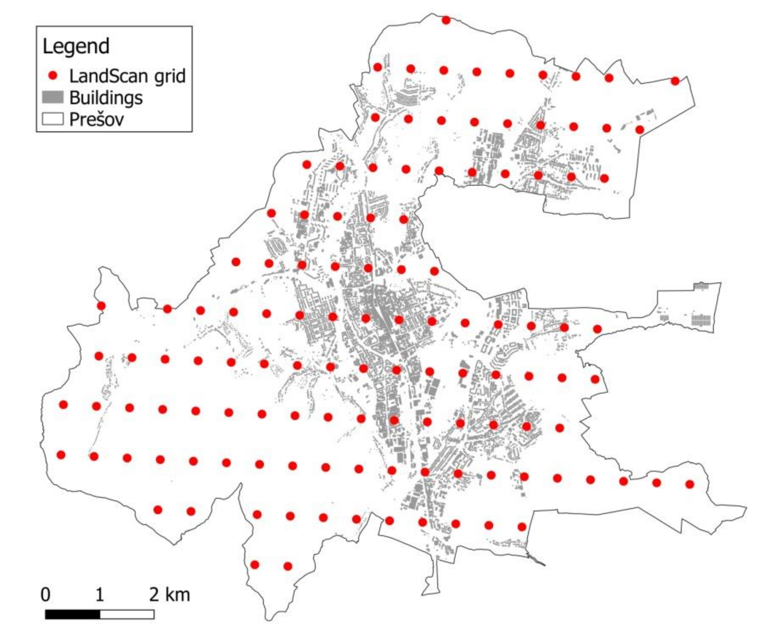
If the historical data on the locations of emergency incidents are not available, the spatial distribution of the demand for EMS must be predicted by a demand model. We investigated two different demand models. The first one is a grid model which takes data from the LandScan database (https://landscan.ornl.gov, accessed on 18 December 2021). LandScan data represents an ambient population distribution, meaning the average presence of people over 24 h. A grid cell corresponds to an area of 30″ × 30″ (arc-seconds) in the WGS84 geographical coordinate system. The population distribution is derived from demographic and geographic data, including land cover, roads, slopes, urban areas, village locations, and high-resolution imagery analyses. Based upon the spatial data and the socioeconomic and cultural understanding of an area, cells are weighted for the possible occurrence of a population during a day. Therefore, the advantage of the ambient spatial model is that it accounts not only for permanent residents, but also for commuters who are not city inhabitants but may need emergency services while they are at work or at school.

The territory of Prešov is covered by 121 grid elements with the population count ranging from 1 to 7827 people, with a median of 79. The centroids of these grid cells are displayed in Figure 2. The nodes of the road networks that are the nearest to the centroids are regarded as demand points.

We assume that the number of patients is proportional to the ambient population. To verify this assumption, we did a correlation analysis between the LandScan population distribution and the real EMS trips performed in 2019 in the city of Prešov. The Spearman correlation is ρ = 0.847, suggesting a strong correlation.

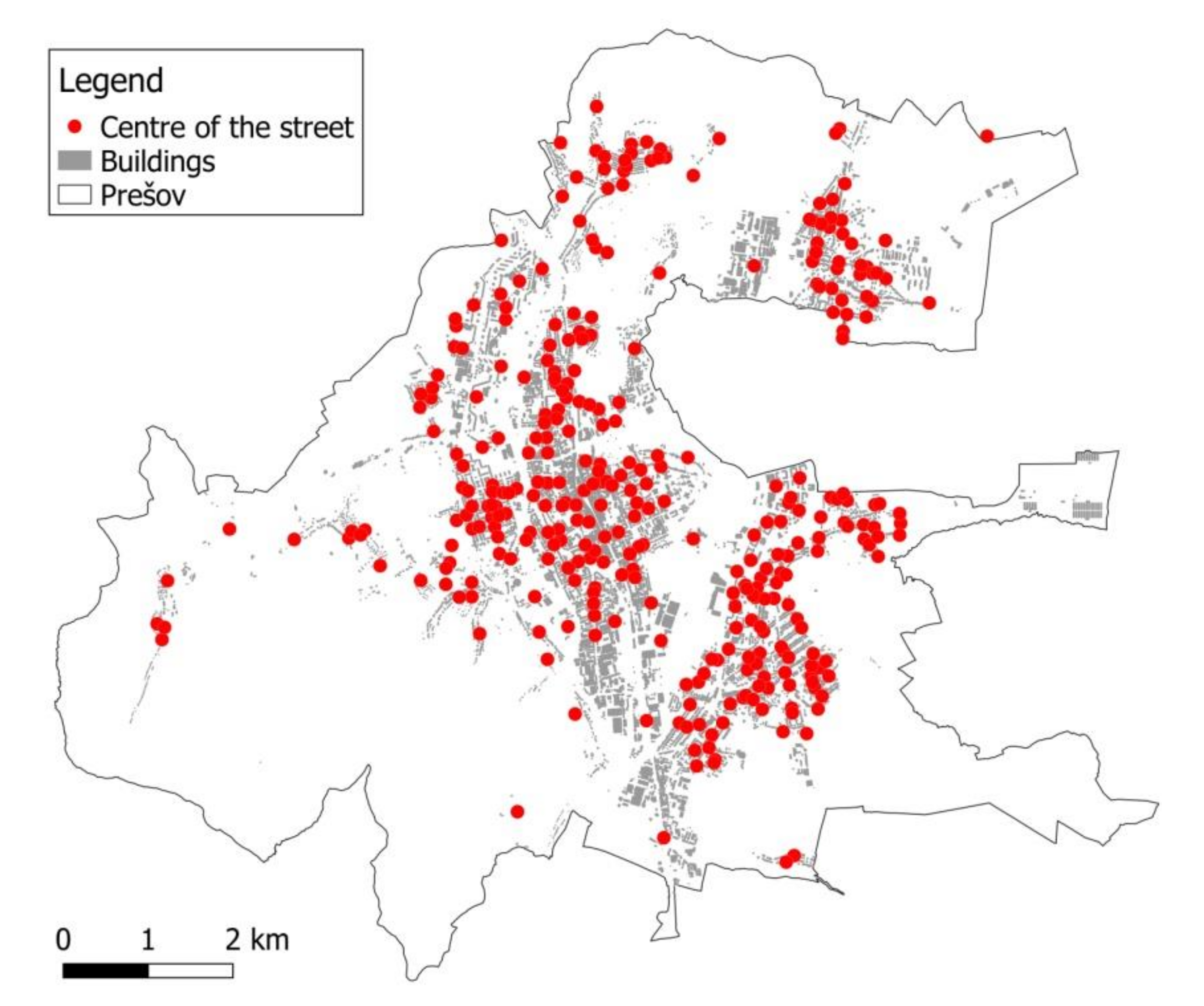
The alternative demand model uses only demographic data on permanent citizens aggregated at a high-resolution level. The local administration regularly updates the number of citizens in every street in the town, which enables us to identify the demand zones within the streets. In 2019, there were 344 streets in Prešov. The number of residents ranged from 0 to 5246 people, with a median of 85. For modelling purposes, the street is represented by its center (Figure 3).

Again, we verified that the demand for EMS is proportional to the number of street residents, using the historical data on EMS trips. The Spearman correlation is ρ = 0.813, still quite strong, although slightly weaker than in the case of the LandScan population.

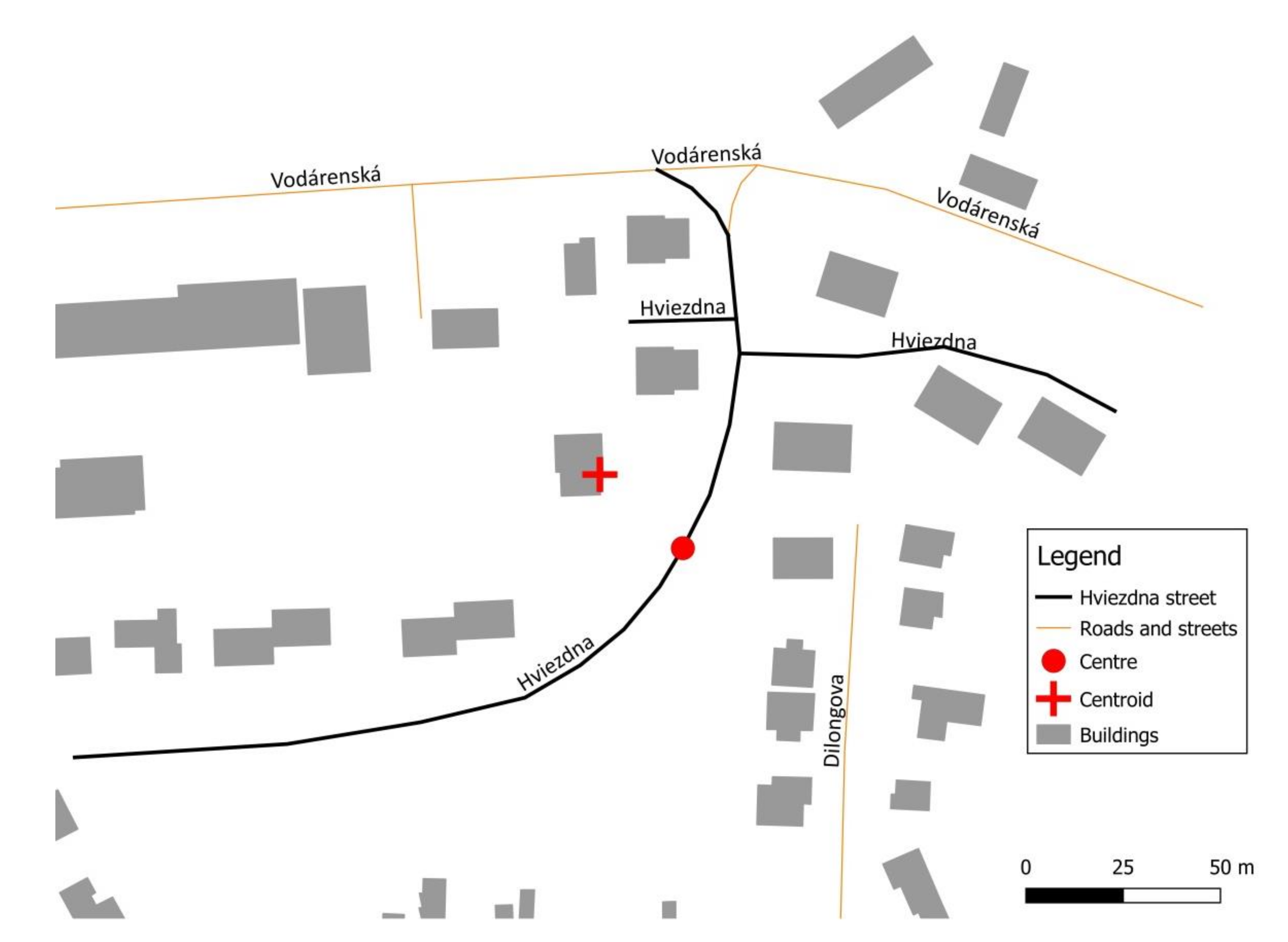
To calculate the center of the street, first we need to determine the centroid (geometric center) of the street. The centroid of the street is the centroid of the envelope enclosing the street. The coordinates of its corners are defined by the extreme points of the polylines that form the street in a digital map. The center of the street is, therefore, the point within the polylines that is nearest to the centroid (Figure 4).

2.7. Setting Parameters in the Location Models

In the pMP, MEXCLP, and ERTM models, the weight b_j of a demand point j corresponds to the ambient population in the grid cell j or the number of people living in the street j, respectively. The MCLP model considers the expected number of patients. The expected numbers b_j1 and b_j2 of high-priority and low-priority patients, respectively, can be calculated using the age structure of the population in the city, and the emergency rates for the particular age categories [29].

Regardless of the demand model, in this study we suppose that candidate locations coincide with demand points. The travel time t_ij is the length (in time units) of the shortest path from node i to node j on the road network. The time an ambulance takes to travel along a road segment depends on the kilometer length of the segment, its quality, its location inside or outside a built-up area, and the average speed of ambulances. The digital street network was downloaded from the OpenStreetMap database (https://www.openstreetmap.org, accessed on 16 April 2019), which is a freely available source of geographical data. All directional, turn, and speed regulations are included in the road network model. For roads without a speed limit, the average travel speed of ambulances, with respect to a given road category, was applied [30]. When an ambulance is driving back to its base station, it rides at a lower speed and respects all traffic regulations. By applying regular speeds, the matrix of longer travel times ${\overline{t}}_{ij}$ can be calculated.

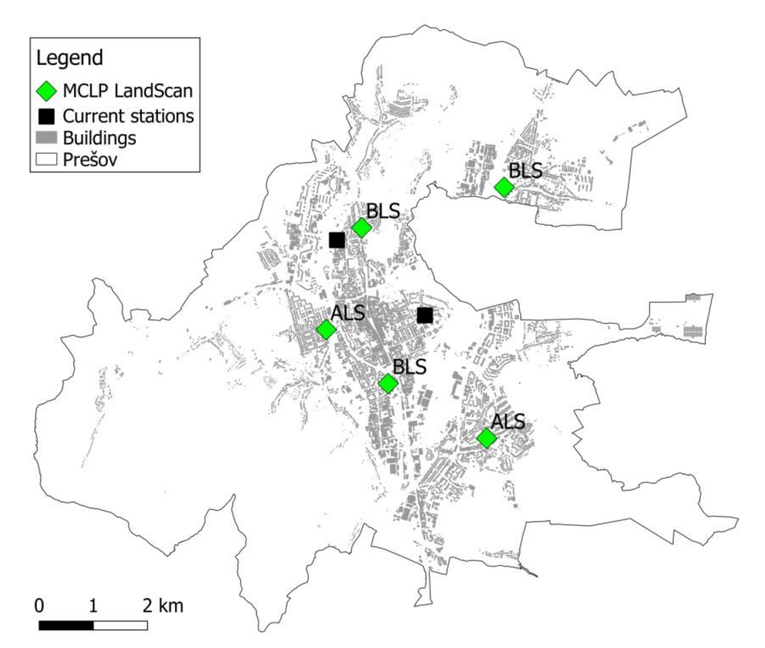
We have the population data valid for the year 2019 at our disposal. Therefore, in the discussion, when talking about the current situation or the current state, we refer to this year. In 2019, there were five stations located at two addresses (e.g., Figure 5). There was one ALS ambulance at each address. The remaining three stations were of a BLS type. Thus, the parameters that specify the number of ambulances in the models are set as follows: p = 5, p₁ = 2, p₂ = 3. If the optimization model does not specify the type of the located stations, we simply assume that the station is of the same type as the closest current station.

The desired service standard $T^{max}$ was set with regard to critical patients who are in a life-threatening condition, and every minute of delay in the response time worsens their chances to survive dramatically. These patients should be reached within 8 min, which is a widely accepted standard in most European countries [31]. Therefore, assuming a one-minute pre-trip delay, we set $T^{max}$ to the value of 7 min. A BLS ambulance cannot be dispatched to priority 1 patients, therefore γ₁₁ = γ₁₂ = γ₂₂ = 1, γ₂₁ = 0.

Most of the coefficients of the MCLP model were derived from an EMS trip sample provided to us by Falck Záchranná a.s., which was the largest EMS provider in Slovakia over the last decade. The Falck dataset contains depersonalized information on 149,474 EMS interventions performed in the year 2015. The age of the patient, their initial medical diagnosis, the type of the intervening ambulance, and the time stamps of the whole EMS trip (including the transport to hospital, if any) have been recorded. Using the data, the parameters were set as follow: α₁ = 50.96%, α₂ = 76.62%, β₁ = 2.51%, β₂ = 6.75%. In Prešov, there is only one hospital. The average drop-off time is td = 20.1 min. The on-scene time depends on the patient’s diagnosis and the crew’s qualification: ts₁₁ = 26.5 min, ts₁₂ = 24.4 min, ts₂₁ = 24.9 min, ts₂₂ = 23 min.

The probability q of an ambulance being unavailable was estimated using a detailed computer simulation model [30]. This microscopic agent-based simulation model was implemented in AnyLogic simulation software and calibrated using the Falck dataset and publicly available statistics published by the National Dispatch Center. The model captures all processes along the emergency care pathway, including reliable distributions of processing times. We simulated the EMS system over the whole country to take into account the fact that ambulances in a town serve not only the city’s citizens but are also used on-demand for the surrounding area, as well as making secondary transportations to more distant hospitals. The probability q of an ambulance being unavailable is calculated as the average workload of all five ambulances operating in the city (q = 38.35%).

3. Results

The distributions of the stations proposed by the location models are evaluated from two viewpoints. The first viewpoint comprises static criteria mostly corresponding to the objective functions of the optimization models. We concentrate on the criteria that are important in practice, and that can also be evaluated in a dynamic environment by means of simulation. The static criteria include:

• Average response time;
• Average expected response time;
• Expected coverage within 15 min;
• Expected coverage within 8 min.

The average response time corresponds to the objective function of the pMP model. It assumes that the closest ambulance is always available, and it is able to respond immediately. The average expected response time is calculated by dividing the objective function of the ERTM model by the total number of potential patients. The expected coverage within 8 min is equal to the objective function of the MEXCLP model. Since the static indicators reflect a simplified system, they can serve as lower and upper bounds for the response time and coverage, respectively.

The second viewpoint includes performance indicators that can be evaluated by means of computer simulation considering all the dynamic and stochastic characteristics of the events that occur in real operations. The main performance indicators are the following:

• Average response time to all patients;
• Percentage of all calls responded to within 15 min;
• Average response time to high-priority patients;
• Percentage of high-priority calls responded to within 8 min.

The percentage of calls responded to within a given time threshold corresponds to the static criteria of the expected coverage.

3.1. Results for the LandScan Demand Model

In this section we evaluate the performance of the location models based on the LandScan distribution of demand in the city of Prešov.

Table 1. Static evaluation of the location models, LandScan model of demand.

Criterion	pMP	MEXCLP Binary	MEXCLP Integer	ERTM	MCLP
Average response time (min)	2.67	3.22	3.74	2.89	2.67
Average expected response time (min)	3.59	3.79	4.01	3.48	3.59
Expected coverage within 15 min (%)	99.08	99.06	99.06	99.07	99.08
Expected coverage within 8 min (%)	97.18	98.34	98.46	97.87	97.18
Computing time (s)	1.13	0.23	0.18	42.94	2.91

presents the static criteria values for the following five models: pMP, MEXCLP with binary location variables, MEXCLP with integer location variables, ERTM, and MCLP. The last row of the table refers to the computing time. The models were solved using the commercial solver Xpress-MP run on a personal computer equipped with an Intel Core i7 processor with 1.60 GHz and 8 GB RAM.

From the static viewpoint, no model outperforms the others unambiguously. The MCLP model results in the same locations of the stations as the pMP model, but proposes a different distribution of ALS and BLS ambulances. However, ambulance types do not affect the static criteria. In general, the models with response time objectives work better than the coverage objective models. Even the expected coverage within the 15 min threshold is better with the pMP, ERTM, and MCLP models than it is with the MEXCLP model. The MEXCLP model with integer variables allocated ambulances to three different station locations. Although its objective function value (the expected coverage within 8 min) is better than that of the MEXCLP model with binary variables, its overall performance is worse.

Computer simulation is supposed to verify whether the dominance of the models with response time objectives holds in practice. The results of the simulation study for the city of Prešov are in

Table 2. Performance indicators for different distributions of the EMS stations in the city of Prešov, LandScan model of demand.

Indicator	Current Locations	pMP	MEXCLP Binary	MEXCLP Integer	ERTM	MCLP
Average response time to all patients (min)	6.12	5.34	5.13	5.30	5.08	5.35
	(6.07; 6.17)	(5.28; 5.40)	(5.03; 5.23)	(5.19; 5.41)	(5.02; 5.15)	(5.24; 5.46)
% of calls responded to within 15 min	95.21	95.22	95.34	95.41	95.30	95.48
Average response times to high-priority patients (min)	5.86	4.64	4.73	5.00	4.56	4.54
	(5.78; 5.93)	(4.51; 4.76)	(4.63; 4.83)	(4.84; 5.15)	(4.47; 4.65)	(4.40; 4.68)
% of high-priority calls responded to within 8 min	88.18	90.96	93.15	93.08	91.90	91.91

. The simulation experiment for one set of station locations consisted of 10 replications. One replication simulated 91 days of EMS performance. For response times, the mean values from 10 replications with 95% confidence intervals are reported. For coverage indicators, the mean values of 10 replications are given. The best values of the indicators are displayed in bold. In the first column, the simulation results for the current distribution of the stations are shown.

As it is demonstrated, all models result in better EMS performance in comparison to the current distribution of the stations. The improvements in the average response times are statistically significant with regard to all patients, as well as to high-priority patients. The best average response time, regardless of the patient’s priority, has been achieved by the ERTM model that reduces the current time by 62 s. The MCLP models exhibits the best improvement in the average response times for high-priority calls (a reduction by 79 s). Since critical patients are of the EMS’s main concern, we consider the MCLP model as the best model from the response time point of view. The locations of the stations proposed by this model are displayed in Figure 5.

Simulated response times are about one minute longer than the expected times produced by mathematical models. The reason behind this is that the simulation model reflects real operations where the ambulances are occupied not only by the calls arising in the city, but also due to the calls coming from the surrounding villages. In addition, secondary transports reduce the ambulance availability as well.

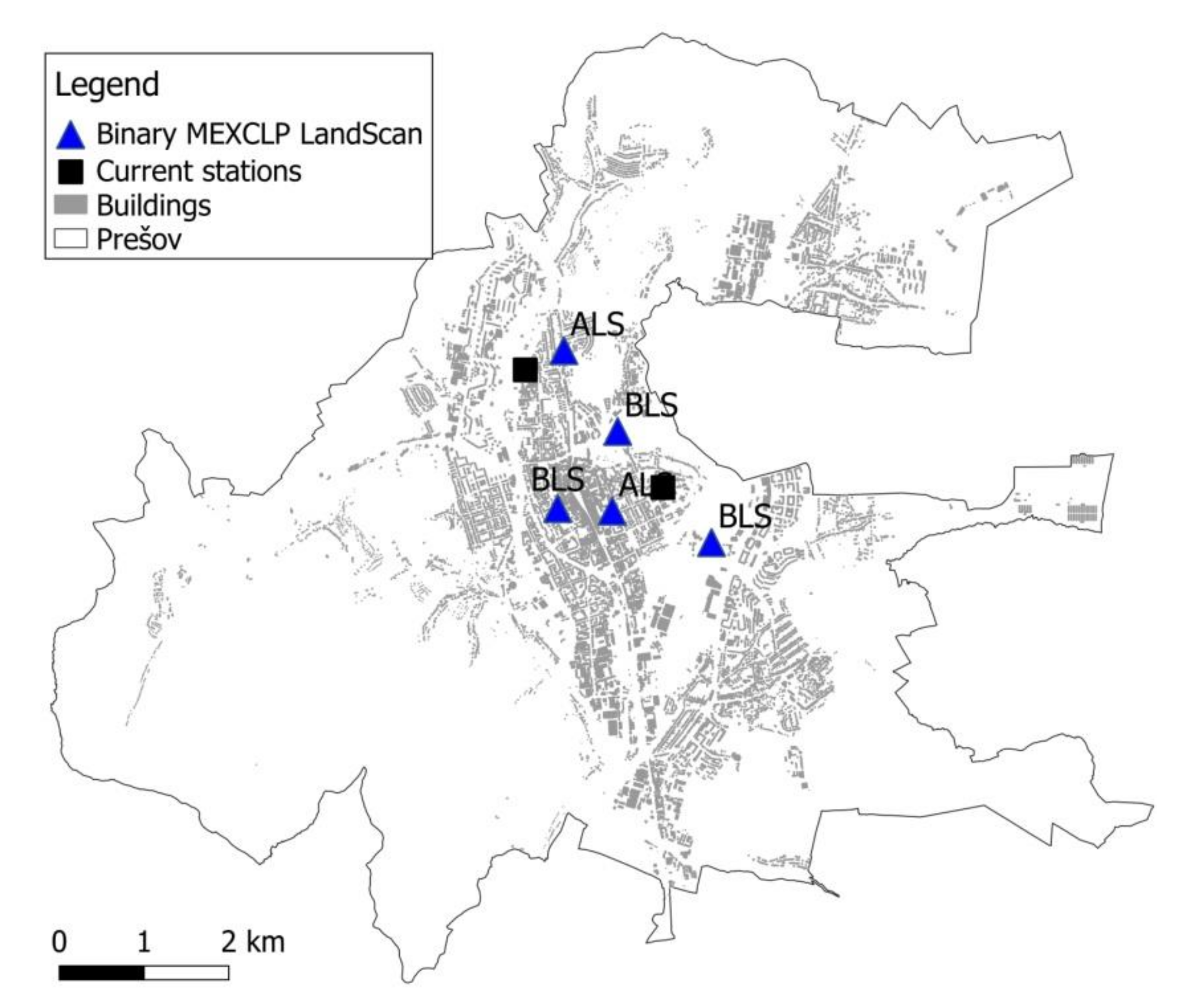
The coverage in the city is very good at present; therefore, the possibilities of location models are limited. The overall coverage meets the national target of reaching 95% of patients within 15 min. The 8-min coverage rate for high-priority calls exceeds the EU average of 66.9% [31]. However, the simulation study has shown that improvements in coverage is still possible, especially regarding high-risk patients. The highest increase in this indicator (by 5%) was achieved by the MEXCLP model with binary variables. This is an unexpected result because the integer MEXCLP outperforms the binary MEXCLP in the static criterion of the 8-min expected coverage. Figure 6 shows that the binary MEXCLP model concentrates the stations close to the city center.

Because the distribution of the stations in the city influences the provision of the services in the surrounding areas, it is wise to also evaluate the performance indicators at the district level. The results of the simulation experiment for the district of Prešov are in

Table 3. Performance indicators for different distributions of the EMS stations in the district of Prešov, LandScan model of demand.

Indicator	Current Locations	pMP	MEXCLP Binary	MEXCLP Integer	ERTM	MCLP
Average response time to all patients (min)	9.60	8.75	8.89	9.04	8.94	8.81
	(9.51; 9.69)	(8.70; 8.80)	(8.76; 9.02)	(8.98; 9.11)	(8.88; 9.00)	(8.72; 8.90)
% of calls responded to within 15 min	83.37	85.87	85.17	85.02	84.78	85.83
Average response time to high-priority patients (min)	9.43	8.38	8.70	8.86	8.60	8.40
	(9.31; 9.55)	(8.33; 8.43)	(8.53; 8.88)	(8.74; 8.99)	(8.44; 8.75)	(8.28; 8.53)
% of high-priority calls responded to within 8 min	51.00	56.34	55.07	53.47	53.86	55.82

. Here we can see that the best improvement was achieved by the pMP model. It is not surprising, because the distribution of the stations in the pMP model is the same as in the MCLP model, and it is more spread out over the city than in the case of the coverage-based models.

3.2. Results for the Street Demand Model

In this section we evaluate the mathematical models where the demand is derived from the permanent residents. The same methodology as in the previous section is applied.

As it shows in the static criteria (

Table 4. Static evaluation of the location models, street model of demand.

Criterion	pMP	MEXCLP Binary	MEXCLP Integer	ERTM	MCLP
Average response time (min)	2.40	3.57	3.71	2.54	2.43
Average expected response time (min)	3.40	4.07	4.18	3.30	3.38
Expected coverage within 15 min (%)	99.37	99.37	99.37	99.37	99.37
Expected coverage within 8 min (%)	95.96	99.07	99.08	97.61	96.01
Computing time (s)	19.39	2.28	2.33	4252.16	138.44

), the results correspond to the theoretical assumptions. The models with response time objectives result in better average response times, while the MEXCLP model is better at the expected coverage within the tighter time limit. The expected 15 min coverage is the same for all models.

The results of the simulation study are in

Table 5. Performance indicators for different distributions of the EMS stations in the city of Prešov, street model of demand.

Indicator	Current Locations	pMP	MEXCLP Binary	MEXCLP Integer	ERTM	MCLP
Average response time to all patients (min)	6.12	5.41	5.06	5.26	5.41	5.56
	(6.07; 6.17)	(5.32; 5.49)	(4.95; 5.16)	(5.17; 5.34)	(5.32; 5.50)	(5.45; 5.67)
% of calls responded to within 15 min	95.21	95.05	95.66	95.45	95.07	94.53
Average response time to high-priority patients (min)	5.86	5.02	4.83	5.04	4.73	4.93
	(5.78; 5.93)	(4.80; 5.25)	(4.71; 4.95)	(4.93; 5.15)	(4.59; 4.88)	(4.74; 5.13)
% of high-priority calls responded to within 8 min	88.18	89.47	91.57	91.70	91.20	90.11

and

Table 6. Performance indicators for different distributions of the EMS stations in the district of Prešov, street model of demand.

Indicator	Current Locations	pMP	MEXCLP Binary	MEXCLP Integer	ERTM	MCLP
Average response time to all patients (min)	9.60	8.97	8.90	8.99	8.95	8.99
	(9.51; 9.69)	(8.92; 9.02)	(8.85; 8.96)	(8.92; 9.06)	(8.86; 9.04)	(8.91; 9.06)
% of calls responded to within 15 min	83.37	85.18	85.13	85.01	85.24	84.92
Average response time to high-priority patients (min)	9.43	8.75	8.72	8.83	8.60	8.67
	(9.31; 9.55)	(8.63; 8.88)	(8.58; 8.87)	(8.73; 8.92)	(8.48; 8.73)	(8.52; 8.82)
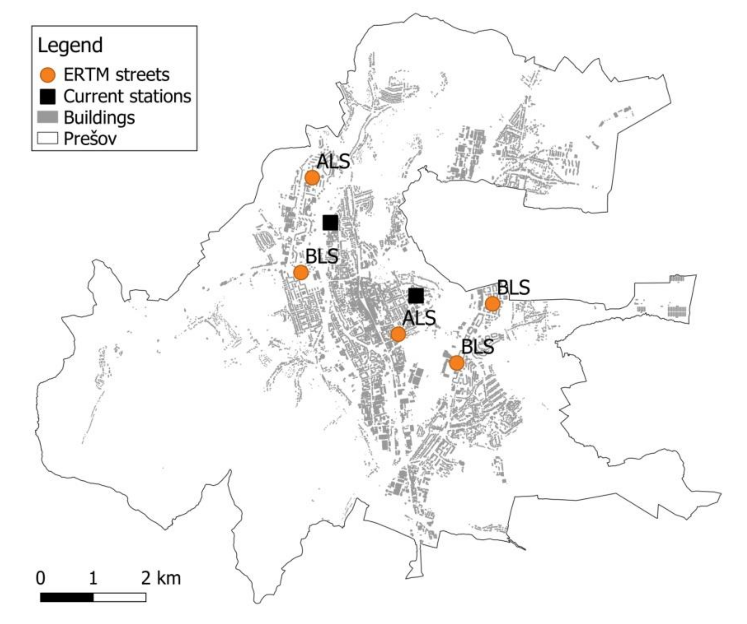
% of high-priority calls responded to within 8 min	51.00	53.48	54.44	53.70	54.23	53.63

for the city and district, respectively. As for the average response time to all patients, the binary MEXCLP model is the best in the city, as well as at the district level, while the ERTM outperforms other models regarding the accessibility to the most critical patients. The distribution of ambulances proposed by two of the most successful binary MEXCLP and ERTM models are in Figure 7 and Figure 8, respectively.

4. Discussion

From the previous analyses it is not clear which location model and demand model propose a network of stations that is likely to ensure the best access to EMS in practice on both levels of spatial resolution (town and district). The confidence intervals of average response times overlap with most models, so they do not prove the superiority of one model over the others. Therefore, we merged the simulated results of all tested location models and both spatial patterns of demand, and then ranked them according to the mentioned performance indicators. The rankings of the models with respect to their simulated performance are in

Table 7. Rankings of the location models with regard to simulated performance.

Area	Indicator	LandScan Model of Demand					Street Model of Demand
		pMP	MEXCLP Binary	MEXCLP Integer	ERTM	MCLP	pMP	MEXCLP Binary	MEXCLP Integer	ERTM	MCLP
City	Average response time to all patients (min)	6	3	5	2	7	8	1	4	8	9
	% of calls responded to within 15 min	7	5	4	6	2	9	1	3	8	10
	Average response time to high-priority patients (min)	3	4	7	2	1	8	5	9	4	6
	% of high-priority calls responded to within 8 min	8	1	2	4	3	10	6	5	7	9
District	Average response time to all patients (min)	1	3	9	5	2	7	4	8	6	8
	% of calls responded to within 15 min	1	5	7	10	2	4	6	8	3	9
	Average response time to high-priority patients (min)	1	5	9	3	2	7	6	8	3	4
	% of high-priority calls responded to within 8 min	1	3	10	6	2	9	4	7	5	8
Total score		28	29	53	38	21	62	33	52	44	63

. The MCLP location model, combined with the LandScan demand model, achieves the best overall score.

In general, the locations of the stations, according to the street demand model, are worse than with the LandScan model. This result was indicated by the correlation analysis between real interventions and demand models, which is slightly tighter for the LandScan model. LandScan population distribution is developed using the best available demographic and geographic data. Moreover, nation-specific socioeconomic and cultural factors are taken into account. The result is the ambient, or average, day/night population distribution that probably better reflects the spatial distribution of emergencies than the permanent residency model. The database is refreshed annually. Thus, we can recommend it as a good model of emergency occurrence in the case of the spatial distribution of emergency incidents when data is not available for the analysis, or the amount of historical data is not sufficient. Our results cannot be confronted with the literature since neither the LandScan model nor the street model have been used yet to estimate the demand for EMS.

Regarding location models, our results are in accordance with previous studies that compared several models. The studies [13,32] compared the models based on the response time and the expected coverage objectives, and concluded that the solution for minimizing the average response time was generally better than the one minimizing the coverage. However, this conclusion is derived only from the analytical evaluation of criteria without considering the stochastic character of a real EMS system by means of simulation. The only simulation study comparing various location models we are aware of is the study by van den Berg and van Essen [6]. In contrast to our research, they did not consider different types of vehicles, and focused only on high-priority patients. Out of the inspected models, the ERTM outperformed the average response time model in most criteria. The MEXCLP performed better than the ERTM in terms of 15 min coverage. Of course, the previous studies do not contain our MCLP model that was proved superior by our experiments. Since this model also minimizes the average response time, our results are compatible with the cited works. The average response time seems to be the most important indicator of EMS access, especially from the most critical patients’ point of view, because it strongly affects the probability of survival for those patients [17,29,33].

The outputs of our study are useful for healthcare providers. We recommend the optimal distribution of ambulances in the city that will increase the responsiveness of EMS. The weak point of our research was that there were no limits on the potential locations of the stations. We suppose that the station can be located at any central node of the LandScan grid, or at any centroid of the street. It was beyond our capabilities to investigate potential locations with all the aspects that have to be taken into account in practical station relocation (i.e., the existence of a proper building, the costs of its tenancy, etc.). Thus, our results should be interpreted in terms of the wards surrounding the calculated optimal station locations rather than stations’ precise addresses. At present, such an interpretation is satisfactory for the decision-makers, as follows from the discussions with the EMS authorities. We note that in practice it may not be acceptable to relocate all stations operating in the city, mainly for economic reasons that are not incorporated into our study. However, the MCLP model, as well as other location models under consideration, can easily cope with such a limitation. It is enough to fix some stations in their current positions by setting corresponding location variables to 1, or by limiting the number of relocated stations by adding a simple constraint to the models.

The results of our study can be applied in all countries with a tiered EMS system that utilizes different types of emergency units, such as dispatching ALS units to the most severe events and using BLS units for non-urgent situations and the scheduled transport of stable patients. Tiered systems apply the Franco-German model of EMS delivery, where the crew is qualified to treat patients in their homes or at the scene. Such systems are common in many European countries such as Germany, France, Greece, Austria, Czech Republic, Hungary, and Poland [34,35,36].

In the future, we will direct efforts to improving the location as well as the demand models. As for the location models, the research will target multiple criteria models. The objectives should balance effectiveness and fairness [32]. Another direction will be oriented towards hierarchical models combining ambulance locations at a macrolevel (across a country or a region) and at a microlevel (cities). Regarding demand models, we will focus on incorporating the surroundings of the city into the demand model, since the ambulances in the city do not serve only the city citizens, but also emergencies arising in neighboring villages.

5. Conclusions

The paper presents a new optimization model for ambulance locations, and a new approach to the modelling demand for EMS in an urban area. The proposed modular capacitated location model is compared to other location models reported in the literature. The case study of the city of Prešov proves that a significant improvement in service quality can be achieved by the optimal distribution of the stations. The following conclusions can be derived from our empirical study:

• The modular capacitated location model outperforms the pMP, MECXLP, and ERTM models.
• The ambient population model better reflects the real spatial distribution of emergency calls compared to the demand model that is based on the permanent residents of the city.