
RiIG Modeled WCP Image-Based CNN Architecture and Feature-Based Approach in Breast Tumor Classification from B-Mode Ultrasound


Abstract
:1. Introduction
- This paper demonstrates the suitability of Rician inverse Gaussian (RiIG) distribution [25] for statistical modeling of the Contourlet transformed breast ultrasound images. Further, it shows that the RiIG distribution is better than the well-known Nakagami distribution in capturing the statistics of Contourlet transformed breast ultrasound images in breast tumors classification.
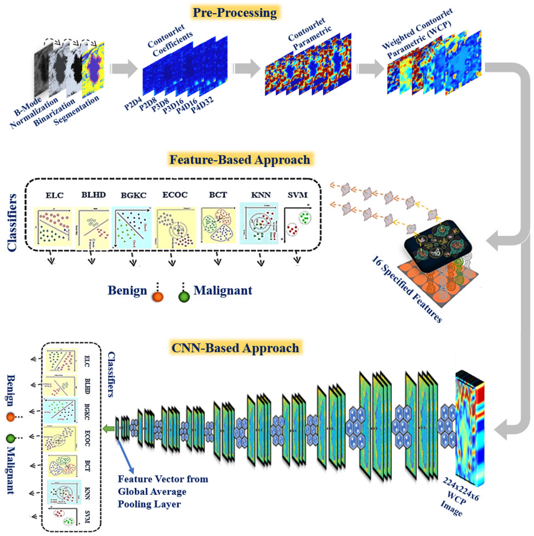
- The suitability of WCP images in classifying breast tumors is investigated for the first time employing three different publicly available datasets consisting of 1193 B-mode ultrasound images and shows that a very high degree of accuracy can be obtained in breast tumor classification using traditional machine-learning-based classifiers as well as deep convolutional neural networks (CNN).
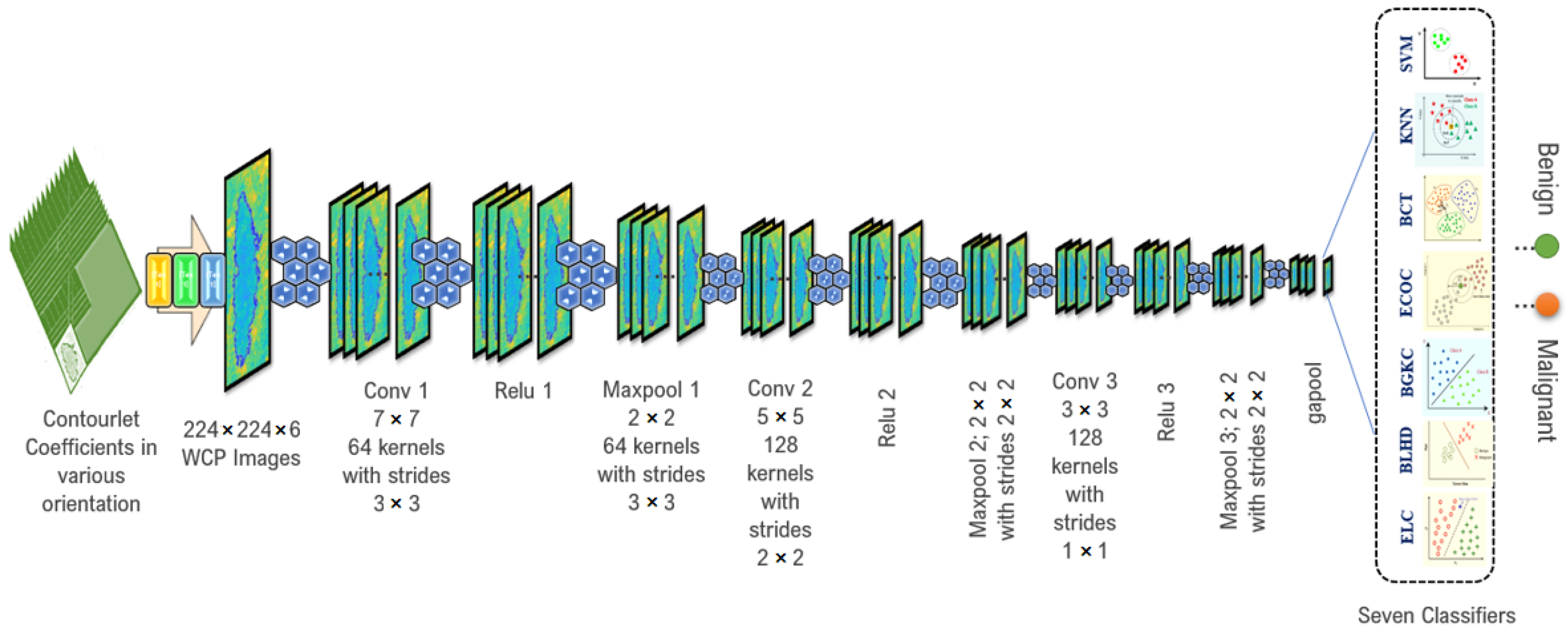
- A new deep CNN architecture is proposed for the classification of breast tumors based on RiIG modeled WCP images for the first time. It is also shown that the efficacy of the CNN architecture is superior to the classical feature-based method.
2. Materials and Methods
2.1. Datasets
2.1.1. Normalization
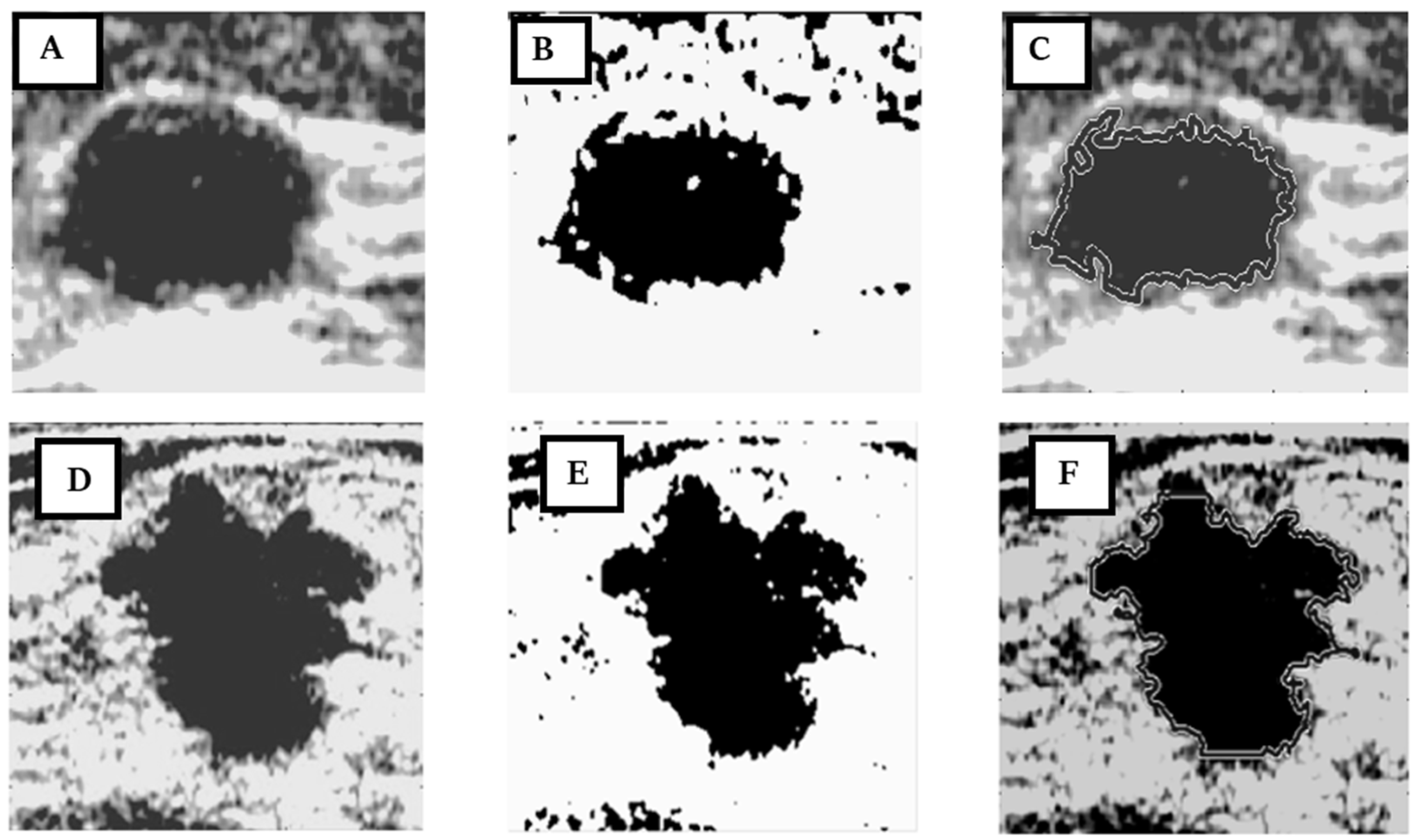
2.1.2. Region of Interest (ROI) Segmentation
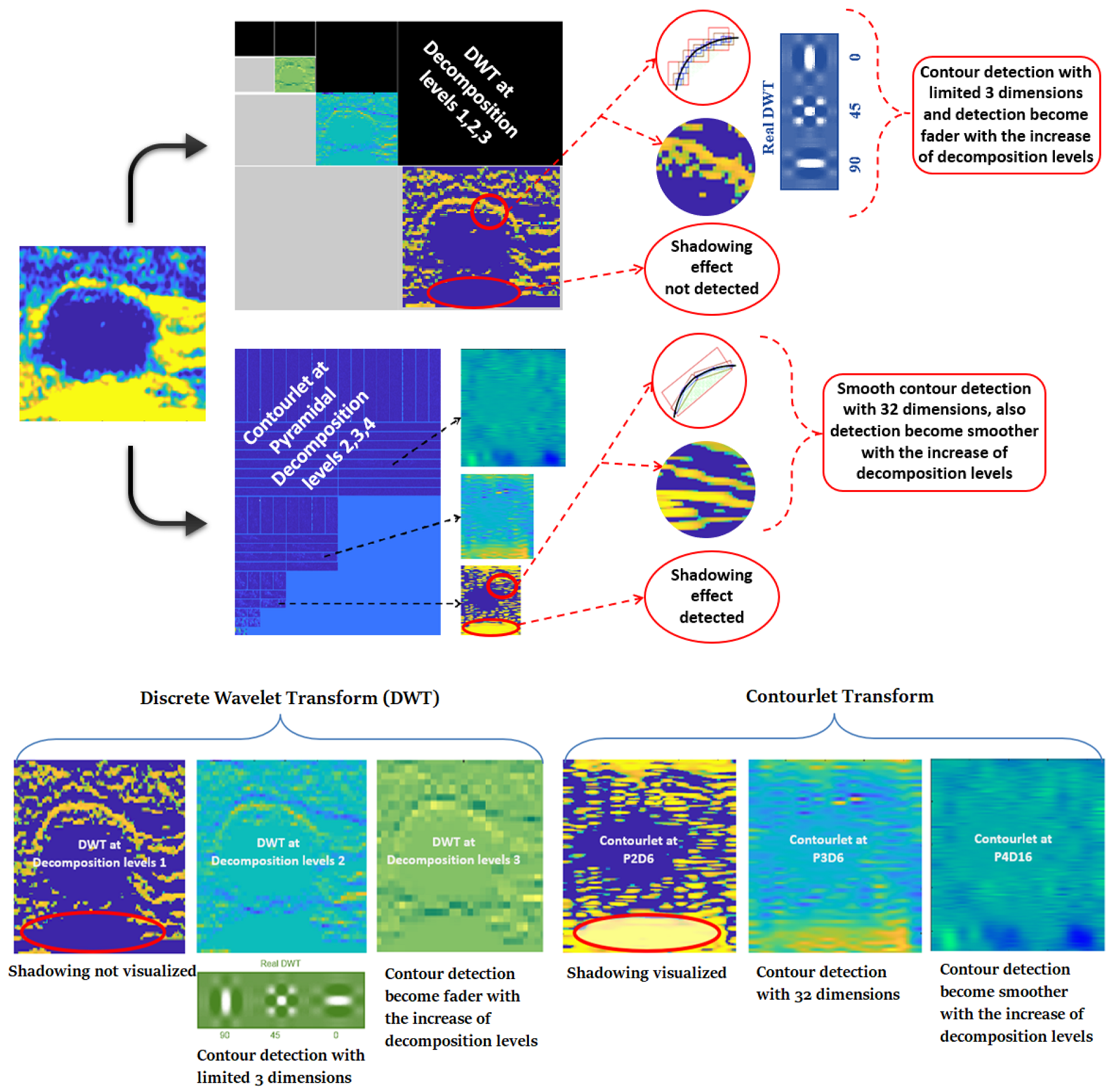
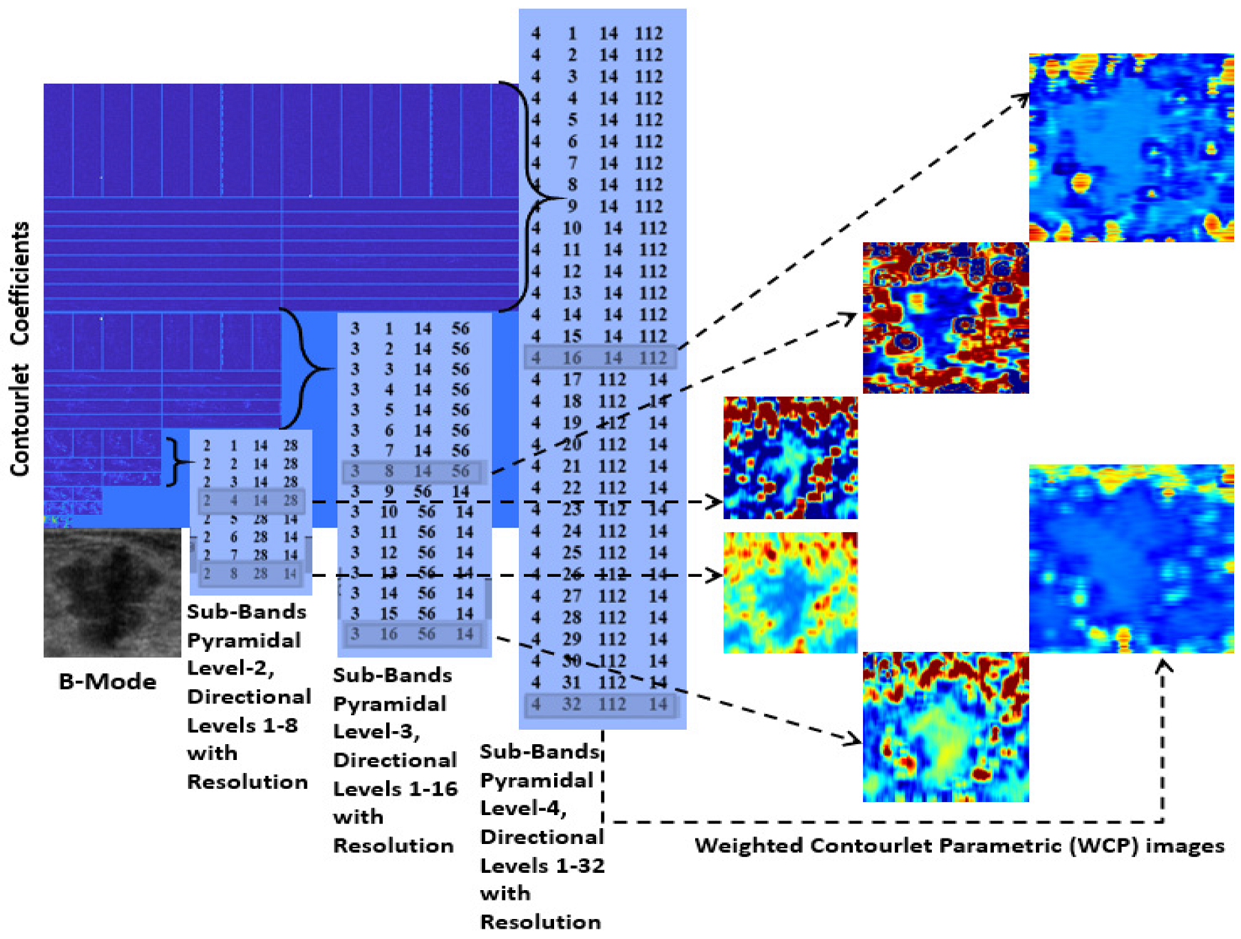
2.1.3. Contourlet Transform
2.1.4. Contourlet Parametric (CP) Image
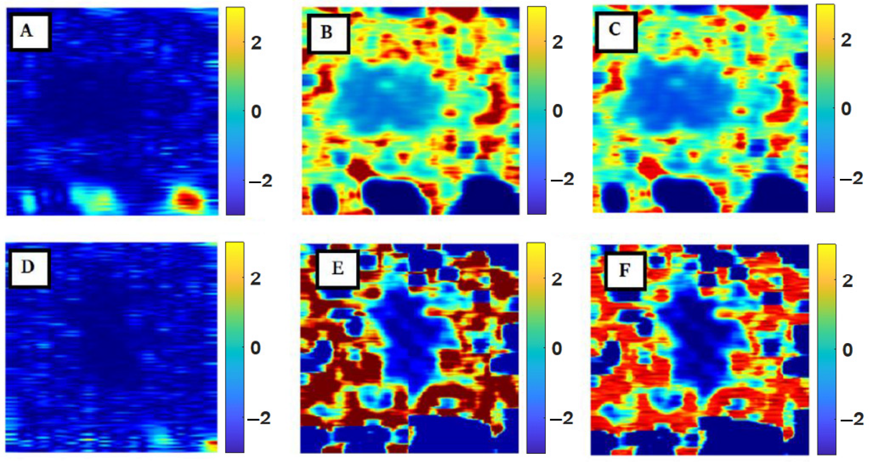
2.1.5. Weighted Contourlet Parametric (WCP) Image
2.2. Feature Extraction
2.3. Proposed Classification Schemes
3. Experimental Results
4. Discussion
5. Conclusions
Author Contributions
Funding
Institutional Review Board Statement
Informed Consent Statement
Data Availability Statement
Conflicts of Interest
References
- Siegel, R.L.; Miller, K.D.; Jemal, A. Cancer statistics, 2020. Cancer J. Clin. 2020, 70, 7–30. [Google Scholar] [CrossRef] [PubMed]
- Horsch, K.; Giger, M.L.; Venta, L.A.; Vyborny, C.J. Computerized diagnosis of breast lesions on ultrasound. Med. Phys. 2002, 29, 157–164. [Google Scholar] [CrossRef] [PubMed]
- Shen, W.-C.; Chang, R.-F.; Moon, W.K.; Chou, Y.-H.; Huang, C.-S. Breast Ultrasound Computer-Aided Diagnosis Using BI-RADS Features. Acad. Radiol. 2007, 14, 928–939. [Google Scholar] [CrossRef] [PubMed]
- Ara, S.R.; Bashar, S.K.; Alam, F.; Hasan, M.K. EMD-DWT Based Transform Domain Feature Reduction Approach for Quantitative Multi-class Classification of Breast Tumours. Ultrasonics 2017, 80, 22–33. [Google Scholar] [CrossRef]
- Acevedo, P.; Vazquez, M. Classification of Tumors in Breast Echography Using a SVM Algorithm. In Proceedings of the International Conference on Computational Science and Computational Intelligence (CSCI), Las Vegas, NV, USA, 5–7 December 2019; pp. 686–689. [Google Scholar] [CrossRef]
- Eltoukhy, M.M.; Faye, I.; Samir, B.B. A comparison of wavelet and curvelet for breast cancer diagnosis in digital mammogram. Comput. Biol. Med. 2010, 40, 384–391. [Google Scholar] [CrossRef]
- Do, M.N.; Vetterli, M. The contourlet transform: An efficient directional multi-resolution image representation. IEEE Trans. Image Process. 2005, 14, 2091–2096. [Google Scholar] [CrossRef] [Green Version]
- Jesneck, J.L.; Lo, J.Y.; Baker, J.A. Breast mass lesions: Computer-aided diagnosis models with mammographic and sonographic descriptors 1. Radiology 2007, 244, 390–398. [Google Scholar] [CrossRef]
- Moayedi, F.; Azimifar, Z.; Boostani, R.; Katebi, S. Contourlet-based mammography mass classification using the SVM family. Comput. Biol. Med. 2010, 40, 373–383. [Google Scholar] [CrossRef]
- Dehghani, S.; Dezfooli, M.A. Breast Cancer Diagnosis System Based on Contourlet Analysis and Support Vector Machine. World Appl. Sci. J. 2011, 13, 1067–1076. [Google Scholar]
- Zhang, Q.; Xiao, Y.; Chen, S.; Wang, C.; Zheng, H. Quantification of Elastic Heterogeneity Using Contourlet-Based Texture Analysis in Shear-Wave Elastography for Breast Tumour Classification. Ultrasound Med. Biol. 2015, 41, 588–600. [Google Scholar] [CrossRef]
- Li, Y.; Liu, Y.; Zhang, M.; Zhang, G.; Wang, Z.; Luo, J. Radiomics with Attribute Bagging for Breast Tumour Classification Using Multimodal Ultrasound Images. J. Ultrasound Med. 2020, 39, 361–371. [Google Scholar] [CrossRef]
- Oelze, M.L.; Zachary, J.F.; O’Brien, W.D. Differentiation of Tumour Types In Vivo By Scatterer Property Estimates and Parametric Images Using Ultrasound Backscatter. In Proceedings of the IEEE Ultrasonics Symposium, Honolulu, HI, USA, 5–8 October 2003; pp. 1014–1017. [Google Scholar] [CrossRef]
- Liao, Y.-Y.; Tsui, P.-H.; Li, C.-H.; Chang, K.-J.; Kuo, W.-H.; Chang, C.-C.; Yeh, C.-K. Classification of scattering media within benign and malignant breast tumours based on ultrasound texture-feature-based and Nakagami-parameter images. J. Med. Phys. 2011, 38, 2198–2207. [Google Scholar] [CrossRef]
- Ho, M.-C.; Lin, J.-J.; Shu, Y.-C.; Chen, C.-N.; Chang, K.-J.; Chang, C.-C.; Tsui, P.-H. Using ultrasound Nakagami imaging to assess liver fibrosis in rats. Ultrasonics 2012, 52, 215–222. [Google Scholar] [CrossRef]
- Bharati, S.; Podder, P.; Mondal, M.R.H. Artificial Neural Network Based Breast Cancer Screening: A Comprehensive Review. Int. J. Comput. Inf. Syst. Ind. Manag. Appl. 2020, 12, 125–137. [Google Scholar]
- Zhou, Y. A Radiomics Approach with CNN for Shear-Wave Elastography Breast Tumor Classification. IEEE Trans. Biomed. Eng. 2018, 65, 1935–1942. [Google Scholar] [CrossRef]
- Zeimarani, B.; Costa, M.G.F.; Nurani, N.Z.; Filho, C.F.F.C. A Novel Breast Tumor Classification in Ultrasound Images, Using Deep Convolutional Neural Network. In Proceedings of the XXVI Brazilian Congress on Biomedical Engineering, Armação de Buzios, Brazil, 21–25 October 2019; pp. 70, 89–94. [Google Scholar] [CrossRef]
- Singh, V.K.; Rashwana, H.A.; Romania, S.; Akramb, F.; Pandeya, N.; Sarkera, M.M.K.; Saleha, A.; Arenasc, M.; Arquezc, M.; Puiga, D.; et al. Breast Tumor Segmentation and Shape Classification in Mammograms using Generative Adversarial and Convolutional Neural Network. Elsevier J. Expert Syst. Appl. 2020, 139, 1–14. [Google Scholar] [CrossRef]
- Ramachandran, A.; Ramu, S.K. Neural network pattern recognition of ultrasound image gray scale intensity histogram of breast lesions to differentiate between benign and malignant lesions: An analytical study. JMIR Biomed. Eng. 2021, 6, e23808. [Google Scholar] [CrossRef]
- Hou, D.; Hou, R.; Hou, J. On-device Training for Breast Ultrasound Image Classification. In Proceedings of the 10th Annual Computing and Communication Workshop and Conference (CCWC), Las Vegas, NV, USA, 6–8 January 2020; pp. 78–82. [Google Scholar] [CrossRef]
- Shin, S.Y.; Lee, S.; Yun, I.D.; Kim, S.M.; Lee, K.M. Joint Weakly and Semi-Supervised Deep Learning for Localization and Classification of Masses in Breast Ultrasound Images. IEEE Trans. Med. Imaging 2019, 38, 762–774. [Google Scholar] [CrossRef] [Green Version]
- Byra, M.; Galperin, M.; Fournier, H.O.; Olson, L.; O’Boyle, M.; Comstock, C.; Andre, M. Breast mass classification in sonography with transfer learning using a deep convolutional neural network and color conversion. Med. Phys. 2019, 46, 746–755. [Google Scholar] [CrossRef]
- Qi, X.; Zhang, L.; Chen, Y.; Pi, Y.; Chen, Y.; Lv, Q.; Yi, Z. Automated diagnosis of breast ultrasonography images using deep neural networks. Med. Image Anal. 2019, 52, 185–198. [Google Scholar] [CrossRef]
- Eltoft, T. The Rician Inverse Gaussian Distribution: A New Model for Non-Rayleigh Signal Amplitude Statistics. IEEE Trans. Image Process. 2005, 14, 1722–1735. [Google Scholar] [CrossRef]
- Rodrigues, S.P. Breast Ultrasound Image. Mendeley Data 2017, 1. [Google Scholar] [CrossRef]
- Yap, M.H.; Pons, G.; Marti, J.; Ganau, S.; Sentis, M.; Zwiggelaar, R.; Davison, A.K.; Marti, R. Automated Breast Ultrasound Lesions Detection using Convolutional Neural Networks. IEEE J. Biomed. Health Inform. 2017, 22, 1218–1226. [Google Scholar] [CrossRef] [Green Version]
- Al-Dhabyani, W.; Gomaa, M.; Khaled, H.; Fahmy, A. Dataset of breast ultrasound images. Data Brief. 2020, 28, 104863. [Google Scholar] [CrossRef]
- Nugroho, H.A.; Triyani, Y.; Rahmawaty, M.; Ardiyanto, I. Breast ultrasound image segmentation based on neutrosophic set and watershed method for classifying margin characteristics. In Proceedings of the 7th IEEE International Conference on System Engineering and Technology (ICSET), Shah Alam, Malaysia, 2–3 October 2017; pp. 43–47. [Google Scholar] [CrossRef]
- Gonzalez, R.C.; Woods, R.E.; Eddins, S.L. Digital Image Processing Using MATLAB, 3rd ed.; Gatesmark Publishing: Knoxville, TN, USA, 2020. [Google Scholar]
- Eltoft, T. Modeling the Amplitude Statistics of Ultrasonic Images. IEEE Trans. Med. Imaging 2006, 25, 229–240. [Google Scholar] [CrossRef]
- Tsui, P.H.; Chang, C.C. Imaging local scatterer concentrations by the Nakagami statistical model. Ultrasound Med. Biol. 2007, 33, 608–619. [Google Scholar] [CrossRef]
- Press, W.H.; Teukolsky, S.A.; Vellerling, W.T.; Flannery, B.P. Numerical recipes in C. In The Art of Scientific Computing; Cambridge University Press: Cambridge, UK, 1999. [Google Scholar]
- Achim, A.; Tsakalides, P.; Bezarianos, A. Novel Bayesian multiscale method for speckle removal in medical ultrasound images. IEEE Trans. Med. Imaging 2001, 20, 772–783. [Google Scholar] [CrossRef] [PubMed] [Green Version]
- Cardoso, J. Infomax and maximum likelihood for blind source separation. IEEE Signal Process. Lett. 1997, 4, 112–114. [Google Scholar] [CrossRef]
- Baek, S.E.; Kim, M.J.; Kim, E.K.; Youk, J.H.; Lee, H.J.; Son, E.J. Effect of clinical information on diagnostic performance in breast sonography. J. Ultrasound Med. 2009, 28, 1349–1356. [Google Scholar] [CrossRef] [PubMed]
- Hazard, H.W.; Hansen, N.M. Image-guided procedures for breast masses. Adv. Surg. 2007, 41, 257–272. [Google Scholar] [CrossRef] [PubMed]
- Balleyguier, V.; Vanel, D.; Athanasiou, A.; Mathieu, M.C.; Sigal, R. Breast Radiological Cases: Training with BI-RADS Classification. Eur. J. Radiol. 2005, 54, 97–106. [Google Scholar] [CrossRef]
- Radi, M.J. Calcium oxalate crystals in breast biopsies. An overlooked form of microcalcification associated with benign breast disease. Arch. Pathol. Lab. Med. 1989, 113, 1367–1369. [Google Scholar]
- Chandrupatla, T.R.; Osler, T.J. The Perimeter of an Ellipse. Math. Sci. 2010, 35, 122–131. [Google Scholar]
- Kabir, S.M.; Tanveer, M.S.; Shihavuddin, A.; Bhuiyan, M.I.H. Parametric Image-based Breast Tumor Classification Using Convolutional Neural Network in the Contourlet Transform Domain. In Proceedings of the 11th International Conference on Electrical and Computer Engineering (ICECE), Dhaka, Bangladesh, 17–19 December 2020; pp. 439–442. [Google Scholar] [CrossRef]
- Kingma, D.P.; Ba, J. Adam: A method for stochastic optimization. In Proceedings of the 3rd International Conference for Learning Representations—ICLR 2015, San Diego, CA, USA, 7–9 May 2015. [Google Scholar]
- Wan, K.W.; Wong, C.H.; Ip, H.F.; Fan, D.; Yuen, P.L.; Fong, H.Y.; Ying, M. Evaluation of the performance of traditional machine learning algorithms. convolutional neural network and AutoML Vision in ultrasound breast lesions classification: A comparative study. Quant. Imaging Med. Surg. 2021, 11, 1381–1393. [Google Scholar] [CrossRef]
- Moon, W.K.; Lee, Y.-W.; Ke, H.-H.; Lee, S.H.; Huang, C.-S.; Chang, R.-F. Computer-aided diagnosis of breast ultrasound images using ensemble learning from convolutional neural networks. Comput. Methods Programs Biomed. 2020, 190, 105361. [Google Scholar] [CrossRef]


| Database-I | |||
| Tumor Type | No. of Patients | No. of Lesions | Method of Confirmation |
| Fibroadenoma (Benign) | 91 | 100 | Biopsy |
| Malignant | 142 | 150 | Biopsy |
Database-II | |||
| Tumor Type | No.ofPatients | No. of Lesions | Method of Confirmation |
| Cyst (Benign) | 65 | 65 | Biopsy |
| Fibroadenoma (Benign) | 39 | 39 | Biopsy |
| Invasive Ductal Carcinoma (Malignant) | 40 | 40 | Biopsy |
| Ductal Carcinoma in Situ (Malignant) | 4 | 4 | Biopsy |
| Papilloma (Benign) | 3 | 3 | Biopsy |
| Lymph Node (Benign) | 3 | 3 | Biopsy |
| Lymphoma (Malignant) | 1 | 1 | Biopsy |
| Unknown (Malignant) | 8 | 8 | Biopsy |
Database-III | |||
| Tumor Type | No. of Patients | No. of Lesions | Method of Confirmation |
| Benign | 600 | 437 | Reviewed by Special Radiologists |
| Malignant | 210 | ||
| Normal | 133 | ||
| Total patients = 996 | Total = 1193 lesions | ||
| PDL | DDL | ANOVA p-Value | PDL | DDL | ANOVA p-Value |
|---|---|---|---|---|---|
| 2 | 1 | 0.077 | 4 | 5 | 0.071 |
| 2 | 2 | 0.054 | 4 | 6 | 0.052 |
| 2 | 3 | 0.078 | 4 | 7 | 0.073 |
| 2 | 4 | 0.022 | 4 | 8 | 0.078 |
| 2 | 5 | 0.066 | 4 | 9 | 0.062 |
| 2 | 6 | 0.066 | 4 | 10 | 0.071 |
| 2 | 7 | 0.062 | 4 | 11 | 0.054 |
| 2 | 8 | 0.018 | 4 | 12 | 0.046 |
| 3 | 1 | 0.076 | 4 | 13 | 0.072 |
| 3 | 2 | 0.081 | 4 | 14 | 0.065 |
| 3 | 3 | 0.074 | 4 | 15 | 0.073 |
| 3 | 4 | 0.045 | 4 | 16 | 0.013 |
| 3 | 5 | 0.054 | 4 | 17 | 0.071 |
| 3 | 6 | 0.063 | 4 | 18 | 0.058 |
| 3 | 7 | 0.058 | 4 | 19 | 0.062 |
| 3 | 8 | 0.008 | 4 | 20 | 0.062 |
| 3 | 9 | 0.055 | 4 | 21 | 0.07 |
| 3 | 10 | 0.065 | 4 | 22 | 0.082 |
| 3 | 11 | 0.079 | 4 | 23 | 0.082 |
| 3 | 12 | 0.067 | 4 | 24 | 0.043 |
| 3 | 13 | 0.071 | 4 | 25 | 0.08 |
| 3 | 14 | 0.065 | 4 | 26 | 0.054 |
| 3 | 15 | 0.062 | 4 | 27 | 0.069 |
| 3 | 16 | 0.025 | 4 | 28 | 0.058 |
| 4 | 1 | 0.073 | 4 | 29 | 0.063 |
| 4 | 2 | 0.058 | 4 | 30 | 0.074 |
| 4 | 3 | 0.068 | 4 | 31 | 0.058 |
| 4 | 4 | 0.048 | 4 | 32 | 0.005 |
| Pyramidal Decomposition Level | Overall Occupied RAM (Capacity 16 GB) | Overall Subband Image Development Time |
|---|---|---|
| 2 | 7.92 GB | 3 min 54 s |
| 3 | 10.89 GB | 6 min 11 s |
| 4 | 13.32 GB | 32 min 36 s |
| 5 | 15.92 GB | 1 h 20 min 43 s |
| Feature with Reference | p-Values |
|---|---|
| Hypoechogenecity [36,37] | 0.0022 |
| Microlobulation [36,37] | 0.0031 |
| Homogeneous Echoes [36,37] | 0.0032 |
| Heterogeneous Echoes [36,37] | 0.0040 |
| Taller Than Wide [36,37] | 0.0044 |
| Microcalcification [38,39] | 0.0054 |
| Texture [38,39] | 0.0069 |
| Shape Class [3] | 0.0145 |
| Echo Pattern Class [3] | 0.0155 |
| Margin Class [3] | 0.0162 |
| Orientation Class [3] | 0.0165 |
| Lesion Boundary Class [3] | 0.0166 |
| Tilted Ellipse Radius [40] | 0.0312 |
| Tilted Ellipse Perimeter [40] | 0.0344 |
| Tilted Ellipse Area [40] | 0.0347 |
| Tilted Ellipse Compactness [40] | 0.0355 |
| Layers | Input Size | Kernel Size | Stride | Output Size |
|---|---|---|---|---|
| Input | 224 × 224 × 6 | |||
| Conv 1 | 224 × 224 × 6 | 7 × 7 × 64 | 3 × 3 | 98 × 98 × 64 |
| Relu 1 | 98 × 98 × 64 | 98 × 98 × 64 | ||
| Maxpool 1 | 98 × 98 × 64 | 2 × 2 × 64 | 2 × 2 | 49 × 49 × 64 |
| Conv 2 | 49 × 49 × 64 | 5 × 5 × 128 | 2 × 2 | 23 × 23 × 128 |
| Relu 2 | 23 × 23 × 128 | 23 × 23 × 128 | ||
| Maxpool 2 | 23 × 23 × 128 | 2 × 2 × 128 | 2 × 2 | 12 × 12 × 128 |
| Conv 3 | 12 × 12 × 128 | 3 × 3 × 128 | 1 × 1 | 10 × 10 × 128 |
| Relu 3 | 10 × 10 × 128 | 10 × 10 × 128 | ||
| Maxpool 3 | 10 × 10 × 128 | 2 × 2 × 128 | 2 × 2 | 5 × 5 × 128 |
| Global Avg. Pool | 5 × 5 × 128 | 1 × 1 × 128 |
| Accuracy (%) with Database-I | |||||||||
| Classifier | B-Mode | B-Mode Parametric | Contourlet | Contourlet Parametric (CP) | Weighted Contourlet Parametric (WCP) | ||||
| Nakagami | RiIG | Nakagami RiIG Nakagami RiIG RiIG (CNN) | |||||||
| SVM | 91.5 | 91.5 | 93.5 | 92 | 91.5 | 93 | 93 | 97.5 | 97.75 |
| KNN | 92 | 91 | 92.5 | 93 | 90.5 | 92 | 92.5 | 95.5 | 98.25 |
| BCT | 88.5 | 90.5 | 91 | 89.5 | 90 | 91.5 | 92.5 | 95 | 96.85 |
| ECOC | 90.5 | 90.5 | 91.5 | 91.5 | 91.5 | 92.5 | 92.5 | 94.5 | 96.45 |
| BGKC | 88 | 89.5 | 90.5 | 89.5 | 89.5 | 90 | 90 | 94 | 95.05 |
| BLHD | 89.5 | 88.5 | 90 | 90.5 | 88.5 | 90.5 | 91.5 | 94.5 | 95.95 |
| ELC | 91 | 92 | 92.5 | 93 | 91.5 | 93 | 93.5 | 96.5 | 97.05 |
Accuracy (%) with Database-II | |||||||||
| Classifier | B-Mode | B-Mode Parametric | Contourlet | Contourlet Parametric (CP) | Weighted Contourlet Parametric (WCP) | ||||
| Nakagami | RiIG | Nakagami RiIG Nakagami RiIG RiIG (CNN) | |||||||
| SVM | 90.50 | 91.95 | 92.25 | 91.40 | 92.90 | 93.15 | 93.95 | 97.55 | 97.90 |
| KNN | 92.05 | 91.85 | 92.00 | 92.65 | 91.10 | 93.05 | 93.55 | 96.30 | 98.35 |
| BCT | 88.35 | 90.05 | 91.35 | 89.55 | 90.45 | 91.85 | 92.55 | 95.05 | 95.75 |
| ECOC | 90.15 | 91.65 | 91.80 | 90.85 | 91.95 | 92.40 | 93.55 | 96.95 | 97.20 |
| BGKC | 87.75 | 88.95 | 90.95 | 88.95 | 89.65 | 90.55 | 90.15 | 94.45 | 95.45 |
| BLHD | 87.15 | 89.20 | 90.55 | 89.20 | 88.25 | 90.05 | 90.75 | 95.05 | 95.15 |
| ELC | 90.20 | 91.45 | 92.05 | 90.55 | 91.55 | 92.15 | 93.10 | 96.95 | 97.65 |
Accuracy (%) with Database-III | |||||||||
| Classifier | B-Mode | B-Mode Parametric | Contourlet | Contourlet Parametric (CP) | Weighted Contourlet Parametric (WCP) | ||||
| Nakagami | RiIG | Nakagami RiIG Nakagami RiIG RiIG (CNN) | |||||||
| SVM | 91.00 | 91.95 | 92.55 | 92.15 | 92.95 | 93.55 | 94.55 | 97.95 | 98.05 |
| KNN | 92.15 | 92.15 | 92.50 | 93.05 | 92.55 | 93.15 | 94.95 | 97.50 | 98.55 |
| BCT | 89.15 | 90.55 | 90.95 | 89.00 | 91.05 | 91.15 | 93.05 | 95.95 | 96.05 |
| ECOC | 90.75 | 92.00 | 92.05 | 91.15 | 92.15 | 92.50 | 94.15 | 97.05 | 97.55 |
| BGKC | 88.15 | 89.05 | 90.55 | 89.05 | 89.95 | 90.15 | 91.15 | 95.15 | 95.55 |
| BLHD | 87.95 | 89.25 | 90.15 | 89.25 | 89.85 | 90.05 | 91.55 | 95.55 | 95.95 |
| ELC | 90.75 | 91.15 | 92.15 | 91.55 | 92.15 | 92.45 | 93.15 | 97.05 | 97.95 |
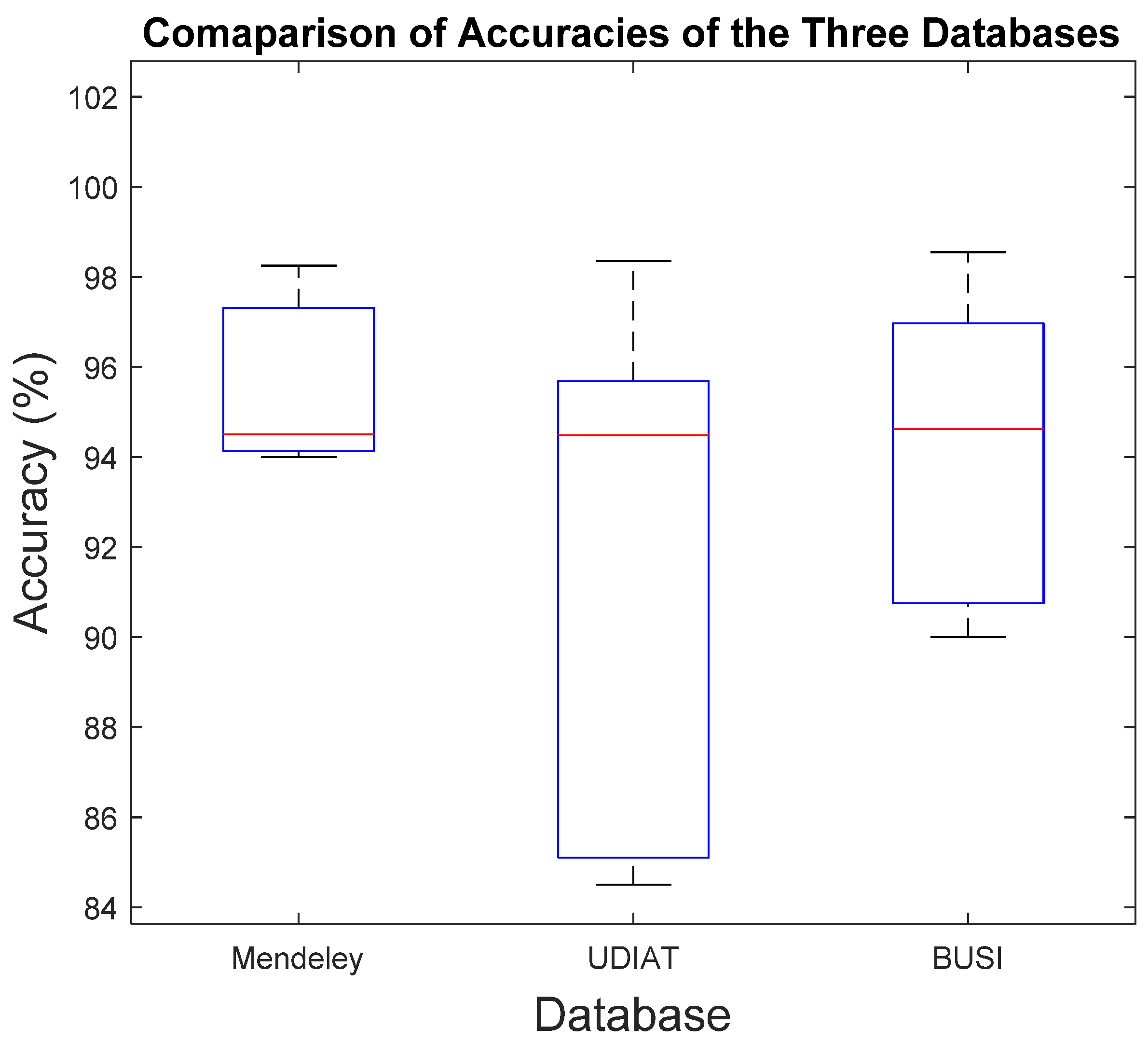
| WCP Image Analysis with Database-I | WCP Image Analysis with Database-II |
 | 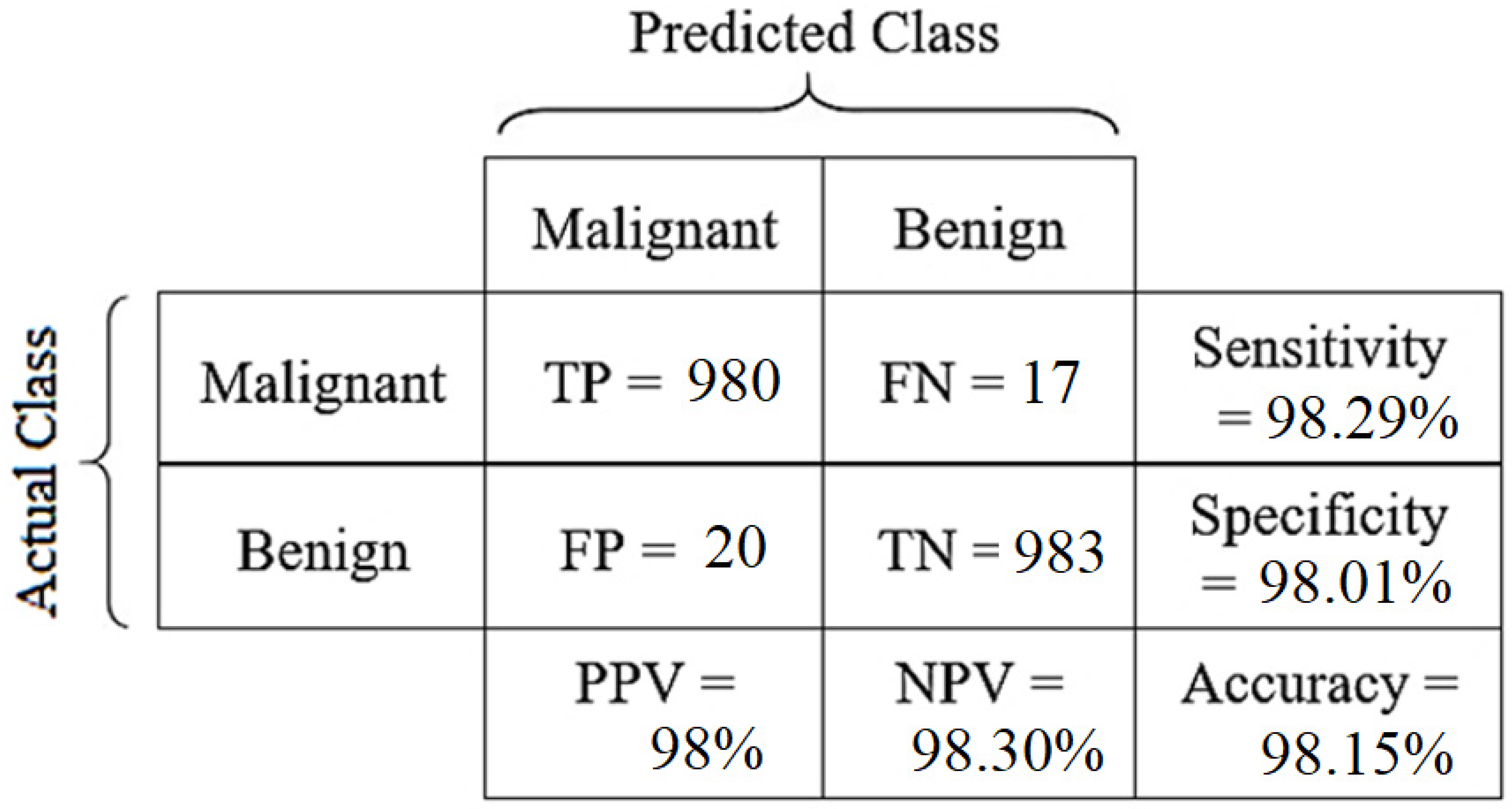 |
| WCP Image Analysis with Database-III | |
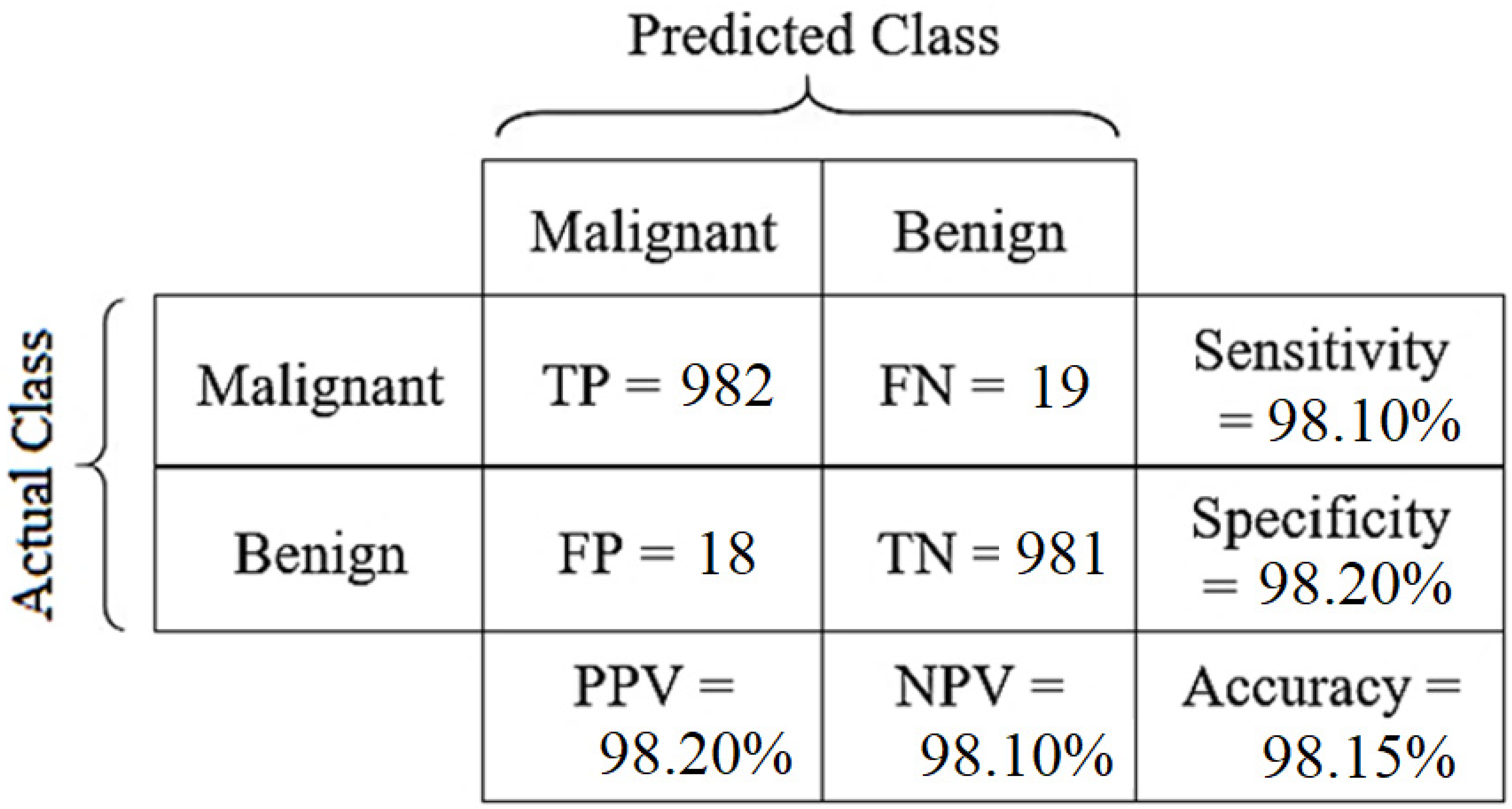 | |
| Author (Year) | Major Contribution | Database | Classifier | Performance (Accuracy in %) |
|---|---|---|---|---|
| P. Acevedo, (2019) [5] | Gray level concurrency matrix (GLCM) algorithm | Database-I [26] | SVM | ACC: 94%, F1 Score: 0.942 |
| Shivabalan K. R. (2021) [20] | Simple Convoluted Neural Network | Database-I [26] | CNN | ACC: 94.5%, SEN: 94.9% SPEC: 94.1%, F1 Score: 0.945 |
D. Hou, (2020), [21] | Portable device-based CNN architecture | Database-II [27] | CNN | ACC: 94.8% |
| S. Y. Shin, (2019) [22] | Neural Network with R-CNN and ResNet-101 | Database-II [27] | R-CNN | ACC: 84.5% |
| M. Byra, (2019) [23] | US to RGB Conversion and fine-tuning using back-propagation | Database-II [27] | VGG19 CNN | ACC: 85.3%, SEN: 79.6% SPEC: 88%, F1 Score: 0.765 |
| X. Qi, (2019) [24] | Deep CNN with multi-scale kernels and skip connections. | Database-II [27] | Deep CNN | ACC: 94.48%, SEN: 95.65% SPEC: 93.88%, F1 Score: 0.942 |
Ka Wing Wan, (2021) [43] | Automatic Machine Learning model (AutoML Vision) | Database-III [28] | CNN Random Forest | ACC: 91%, SEN: 82% SPEC: 96%, F1 Score: 0.87 ACC: 90%, SEN: 71% SPEC: 100%, F1 Score: 0.83 |
| Woo Kyung Moon, (2020) [44] | CNN includes VGGNet, ResNet, and DenseNet. | Database-III [28] | Deep CNN | ACC: 94.62%, SEN: 92.31% SPEC: 95.60%, F1 Score: 0.911 |
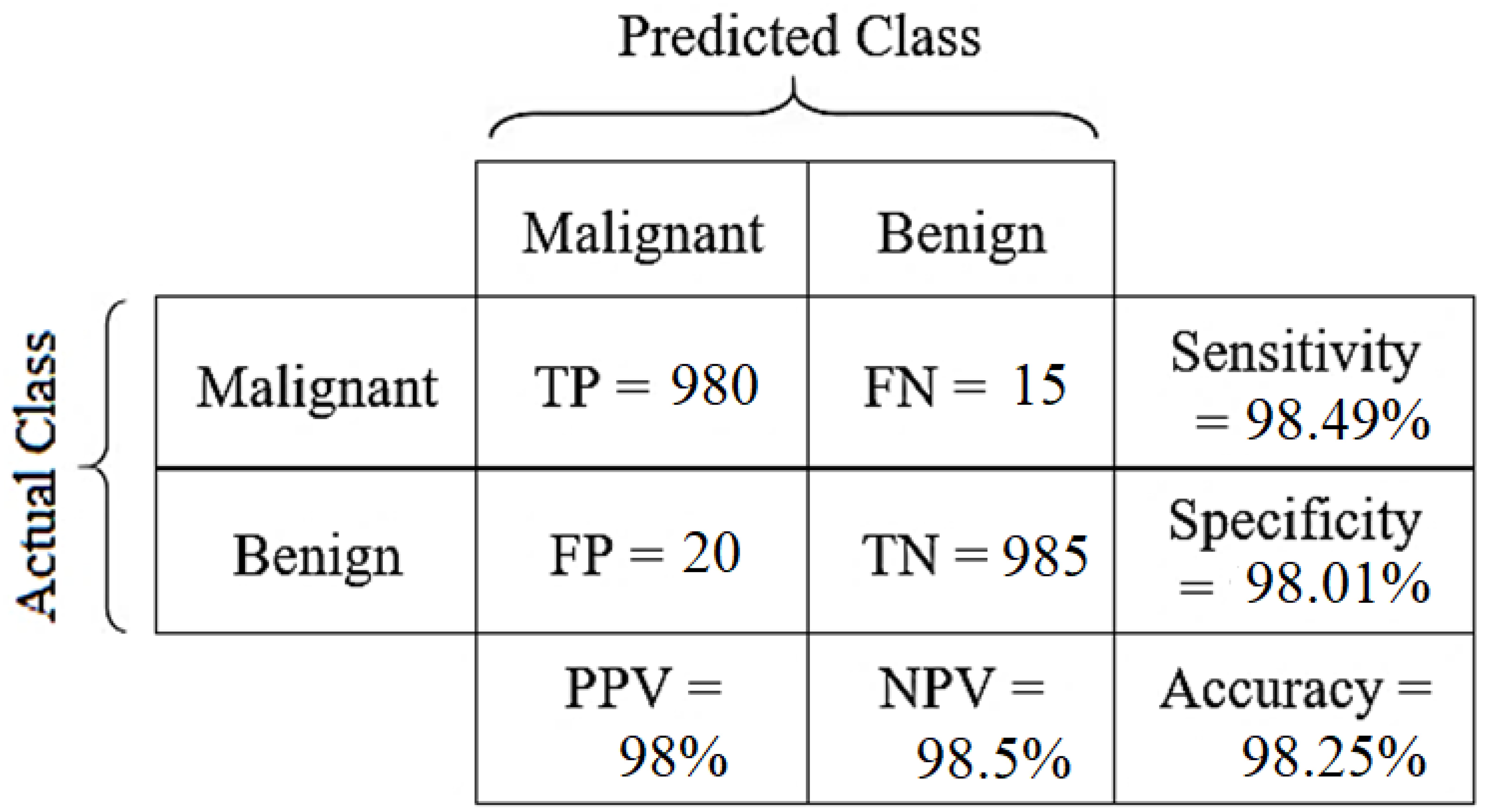
| Proposed Method | WCP Image, Custom made CNN architecture | Database-I [26] | Deep CNN | ACC: 98.25%, SEN: 98.49% SPEC: 98.01%, F1 Score: 0.982 |
| Database-II [27] | Deep CNN | ACC: 98.35%, SEN: 98.11% SPEC: 98.59%, F1 Score: 0.984 | ||
| Database-III [28] | Deep CNN | ACC: 98.55%, SEN: 98.21% SPEC: 98.89%, F1 Score: 0.986 |
Publisher’s Note: MDPI stays neutral with regard to jurisdictional claims in published maps and institutional affiliations. |
© 2021 by the authors. Licensee MDPI, Basel, Switzerland. This article is an open access article distributed under the terms and conditions of the Creative Commons Attribution (CC BY) license (https://creativecommons.org/licenses/by/4.0/).
Share and Cite
Kabir, S.M.; Bhuiyan, M.I.H.; Tanveer, M.S.; Shihavuddin, A. RiIG Modeled WCP Image-Based CNN Architecture and Feature-Based Approach in Breast Tumor Classification from B-Mode Ultrasound. Appl. Sci. 2021, 11, 12138. https://doi.org/10.3390/app112412138
Kabir SM, Bhuiyan MIH, Tanveer MS, Shihavuddin A. RiIG Modeled WCP Image-Based CNN Architecture and Feature-Based Approach in Breast Tumor Classification from B-Mode Ultrasound. Applied Sciences. 2021; 11(24):12138. https://doi.org/10.3390/app112412138
Chicago/Turabian StyleKabir, Shahriar Mahmud, Mohammed I. H. Bhuiyan, Md Sayed Tanveer, and ASM Shihavuddin. 2021. "RiIG Modeled WCP Image-Based CNN Architecture and Feature-Based Approach in Breast Tumor Classification from B-Mode Ultrasound" Applied Sciences 11, no. 24: 12138. https://doi.org/10.3390/app112412138
APA StyleKabir, S. M., Bhuiyan, M. I. H., Tanveer, M. S., & Shihavuddin, A. (2021). RiIG Modeled WCP Image-Based CNN Architecture and Feature-Based Approach in Breast Tumor Classification from B-Mode Ultrasound. Applied Sciences, 11(24), 12138. https://doi.org/10.3390/app112412138