Prediction of Subsidence during TBM Operation in Mixed-Face Ground Conditions from Realtime Monitoring Data

Abstract

The prediction of settlement during tunneling presents multiple challenges, as such settlement is governed by not only the local geology but also construction methods and practices, such as tunnel boring machine (TBM). To avoid undesirable settlement, engineers must predict the settlement under given conditions. The widely used methods are analytical solutions, empirical solutions, and numerical solutions. Analytical or empirical solutions, however, have limitations, which cannot incorporate the major causes of subsidence, such as unexpected geological conditions and TBM operational issues, among which cutterhead pressure and thrust force-related factors are the most influential. In settlement prediction, to utilize the machine data of TBM, two phases of long short-term memory (LSTM) models are devised. The first LSTM model is designed to capture the features affecting surface settlement. The second model is for the prediction of subsidence against the extracted features. One thing to note is that predicted subsidence is the evolution of settlement along TBM drive rather than its maximum value. The proposed deep-learning models are capable of predicting the subsidence of training and test sets with excellent accuracy, anticipating that it could be an effective tool for real-world tunneling and other underground construction projects.

1. Introduction

Underground construction using Tunnel Boring Machines (TBMs) is rapidly increasing to meet demands for new roads, railways, and electrical and telecommunication infrastructure associated with rapid urbanization. The TBM method offers several advantages, such as closed-mode operations, over other traditional approaches in terms of the safety measures involved in applying face-support pressures and the instant support provided by concrete linings, which mitigate the risks posed by the high groundwater pressure under water table.

Mixed-face ground conditions during TBM driving pose the most challenging risks. The soft soil at the top of the face and the hard rock at the bottom makes it difficult to maintain a proper face-support pressure and face stability, and increases the risk of excessive cutter wear, face collapse, sinkholes, or damage to surrounding structures [1]. To avoid undesirable settlement and provide appropriate safety measures, engineers must reliably predict the amount of settlement under given ground conditions. The most widely accepted analytic solution, proposed by Peck [2], is based on measurements from various projects and has been modified to apply to TBM excavations in geologically mixed-face conditions for metropolitan projects in the congested urban area [3].

However, an analytic solution has its own limitations, as it may not be able to incorporate the important causes of subsidence, such as unexpected geological conditions and subsequent ground deformation, over-excavation, untreated tail voids, curvature with a short radius, and TBM operational issues, including chamber pressure, penetration or advance rate, muck volume, torque, and thrust force. Cutterhead face pressure and thrust force related factors are most influential among these issues [4].

The project, in this study, involves a mixed-face condition of alluvial and weathered soil, weathered rock, and soft rock from the top to the bottom of the tunnel face throughout the length of a tunnel. A previous study found that machine learning with geological information without TBM data generated poor settlement estimates [5]. We hypothesized that the correlation of key parameters, such as thrust force and advance rate, with respect to the amount of settlement would lead to an improved theoretical framework, as we analyzed more TBM data.

In this paper, a series of LSTM models are adopted, where the first LSTM model extracted hidden features that could affect ground movement/subsidence, and the second LSTM model was trained for the prediction of the subsidence against the hidden features obtained from the earlier model. 10,660,000 TBM measurements and settlement data from 48 settlement markers were collected and fed into a long short-term memory (LSTM) model. After several weeks of training and testing, the LSTM models demonstrated excellent performance of subsidence prediction for both the training and test cases, indicating significant advances in the reliable prediction of subsidence against pure machine data.

2. Literature Review

Analytical, empirical, and numerical methods have been widely used to estimate the amount of settlement caused by tunnel excavations. Peck [2] proposed a very well-known empirical solution using an inverted Gaussian distribution curve, as shown in Figure 1. Several variations of the empirical solution have been applied [6,7]. Although empirical solutions are easy to apply, they can only accommodate a handful of factors out of the various factors shown in Figure 2, and often exclude various temporally and spatially relevant factors, such as localized geological structures and an advance rate [8,9].

Analytical solutions based on soil and rock mechanics, which are also easy to apply and enjoy a comparable academic foundation, also suffer from similar limitations. Numerical methods offer advantages over other empirical or analytical methods to build models that accommodate the constitutive equations, geological layers, localized geological structures, and construction sequences. However, they require the elaboration of time-consuming models in addition to the uncertainty of geotechnical properties [10]. To tackle these issues and to resolve the non-linear relationship between ground reactions and subsidence, the various AI models and machine-learning (ML) approaches have been applied using data from the sensors of a TBM [5,11,12,13] as summarized in

Table 1. AI models for predicting surface settlement induced by tunneling.

AI Model	Researcher	Theme	Year
PCA/ANFIS	Bouayad, D; Emeriault, F. [12]	Ground surface settlements induced by shield tunneling	2017
Evolutionary Hybrid Neural Network	Zhang, K.; Lyu, H. M.; Shen, S. L.; Zhou, A.; Yin, Z. Y. [5]	Predicting shield tunneling induced ground settlement	2020
Machine Learning	Chen, R.; Zhang, P.; Wu, H.; Wang, Z.; Zang, Z. [13]	Predicting shield tunneling induced ground settlement	2019
ANN (Artificial Neural Network)	Kim, C.; Bae, G.; Hong, C.; Park, S.; Shin, H. [14]	Prediction of ground surface settlement due to tunneling	2001
	Suwansawat, S.;Einstein, H. [15]	Prediction the max. surface settlement caused by EPB Shield	2006
PSO-ANN	Hasanipanah, M.; Nooria-Bidgoli, M.; Jahed Armaghani, D.; Khamesi, H. [16]	Predicting surface settlement caused by tunneling	2016
SVM (Support Vector Machine)	Samui, P. Sitharam, T. [17]	Settlement of shallow foundation on cohesionless soil	2008

.

Machine-learning algorithms have become increasingly popular with the advent of deep-learning (DL) algorithms. Many attempts to apply ML to geotechnical problems were made even before the advent of DL. Examples include artificial neural networks (ANNs) [14,15,18], adaptive neuro fuzzy-based inference (ANFIS) [12], decision trees (DT) [19], back-propagation neural networks (BPNNs) [15,20,21], support vector minimization (SVM) [17], and gated recurrent units (GRU) [22].

To estimate subsidence, Samui and Sitharam adopted a hybrid approach using an ANN model reinforced by a differential evolutionary algorithm [17]. Similarly, Kim and Lee adopted ANN for the assessment of risks of abandoned mine subsidence [23]. Chen et al. and Zhang et al. applied various ML and DL algorithms, including a BPNN, wavelet neural network (WNN), logistic regression, extreme learning machine (ELM), SVM, and random forests (RF) to estimate the maximum subsidence due to tunnel excavation, however, the estimation of maximum settlement with AI is hardly more valuable than analytical, empirical or numerical methods [13].

Some of the common problems of small datasets are over-fitting and the poor performance of models when it comes to applying them to real world problems, as the model is trained on a subset of real-world conditions. The simple comparison of various methods does not always provide much value, as each method requires extensive effort, skill, and expertise for the best performance.

One of the advantages of using the DL, such as LSTM, is self-feature analysis; provided the volume of the data is sufficiently large and the model is deep enough, then denoise steps can be omitted without affecting the model’s performance. On the other hand, if the data is pre-processed too small, because of difficulty of handling a large dataset, and its features were selected by the engineer, then the chances of overfitting and degradation of model performance increase.

3. Description of Project and EPB (Earth Pressure Balance) TBM Driving

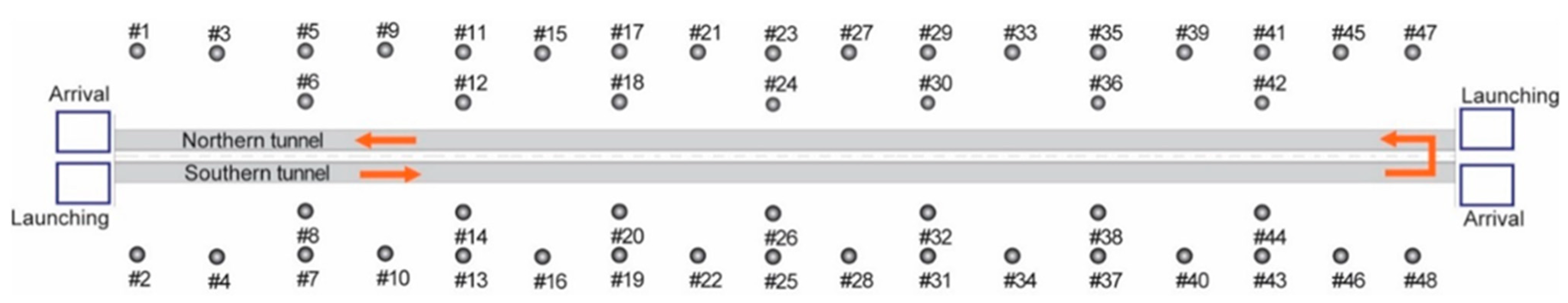
3.1. TBM Driving

The EPB- (Earth Pressure Balance) type TBM data were obtained from a metropolitan project in downtown Seoul. The tunnel is 1600 m long and consisted of two stations and seven ventilation shafts. The lengths of alignment for the lot were 370 m and 373 m for the northern and southern tunnels, respectively, and a total of 498 segment rings were installed. One EPB TBM was used for both single-track twin tunnels, for a total excavation length of 743 m. The tunnel was relatively shallow, at approximately 12 to 15 m, and the ground at the departure zone was composed of a mix of weathered rock and soft rock, while the ground at the arrival zone consisted of alluvial soil. The groundwater level was approximately 7 to 8 m below the surface and 3 to 4 m above the tunnel crown. To monitor the amount of settlement during EPB TBM excavation, 48 settlement markers were installed along the alignment.

Table 2. EPB TBM details.

Item	Description
Type	Earth pressure balance
Supplier	Herrenknecht (Germany)
OD/ID	7.71 m/7.69 m
Thrust force	1154 kN/m2/53,878 kN
Cutter head	Dome type, 17-inch cutter, scraper
Torque	10,364–6500 kN-m (α = 22~25)
RPM	3.4 RPM, electric motor type
Segment	RC-segment, L1, 500 mm + t300 mm, 7 pieces
Muck handling	Muck car + vertical conveyor belt, belt scale
Grouting	Upper Section 4 EA, probe drilling (22 holes)

provides the dimensions and specifications of the EPB TBM used in the project.

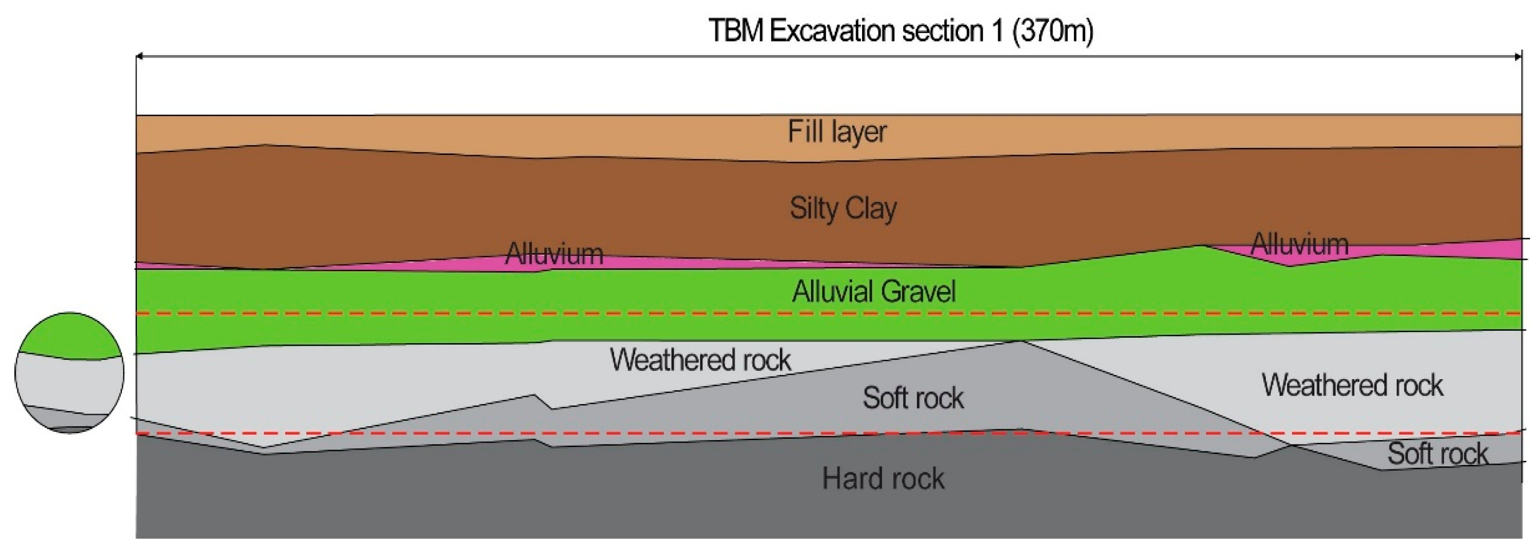
3.2. Geological Site Conditions

Table 3. Geological site conditions.

Item	Characteristics of Rock Type
Residual soil	Sandy gravel, N: 3~50, max size: φ500 mm
Weathered rock	Silty core, Cohesion: 31 kPa, φ = 32°
Soft rock	Gneiss, RMR: 30~50
Water Level	Approx. GL-7 m
Unit weight	20–21 kN/m2
UCS	20–110 MPa
Permeability	2.5 × 10−3~2.5 × 10−5 cm/s

summarizes the typical geological condition along the alignment of the tunnel. Figure 3 depicts the geological layout of the alignment. At tunnel depth, the construction site’s geology is a mixed face condition, consisting of alluvial gravel at the crown, weathered rock at the middle, and soft to hard rock at the bottom of the tunnel face. This mixed-face condition is unfavorable in terms of face stability, and the risk of settlement was high due to the potential for over-excavation at the crown, whereas the bottom section retarded the advance of the TBM.

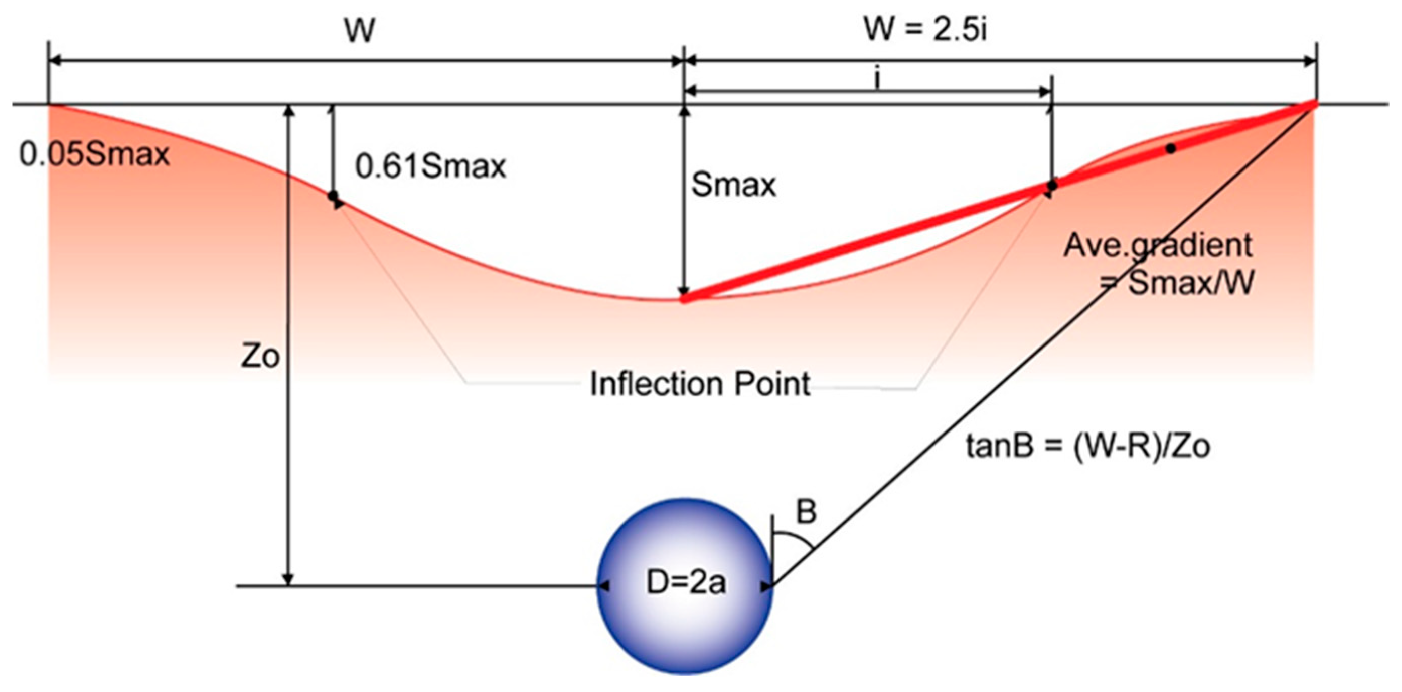
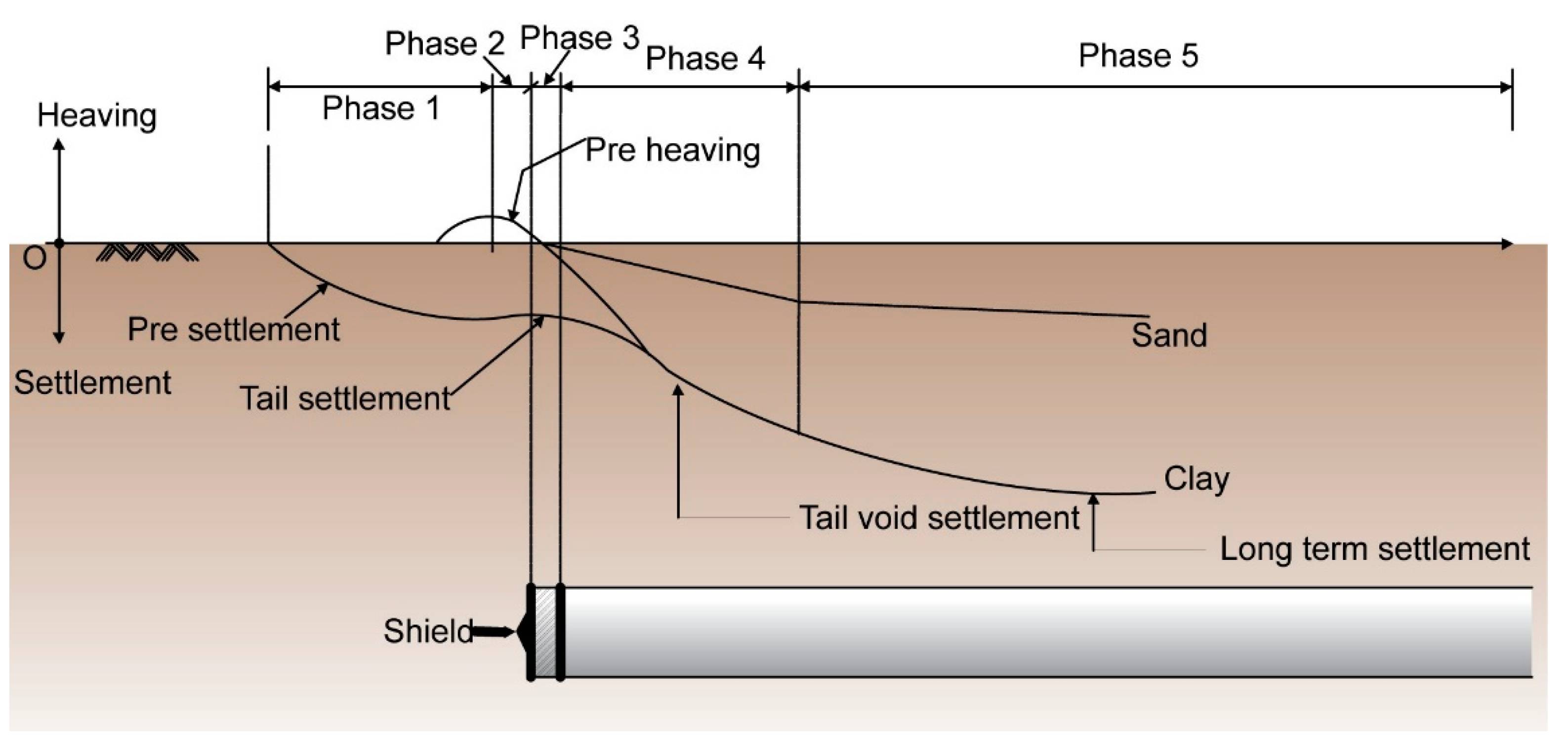
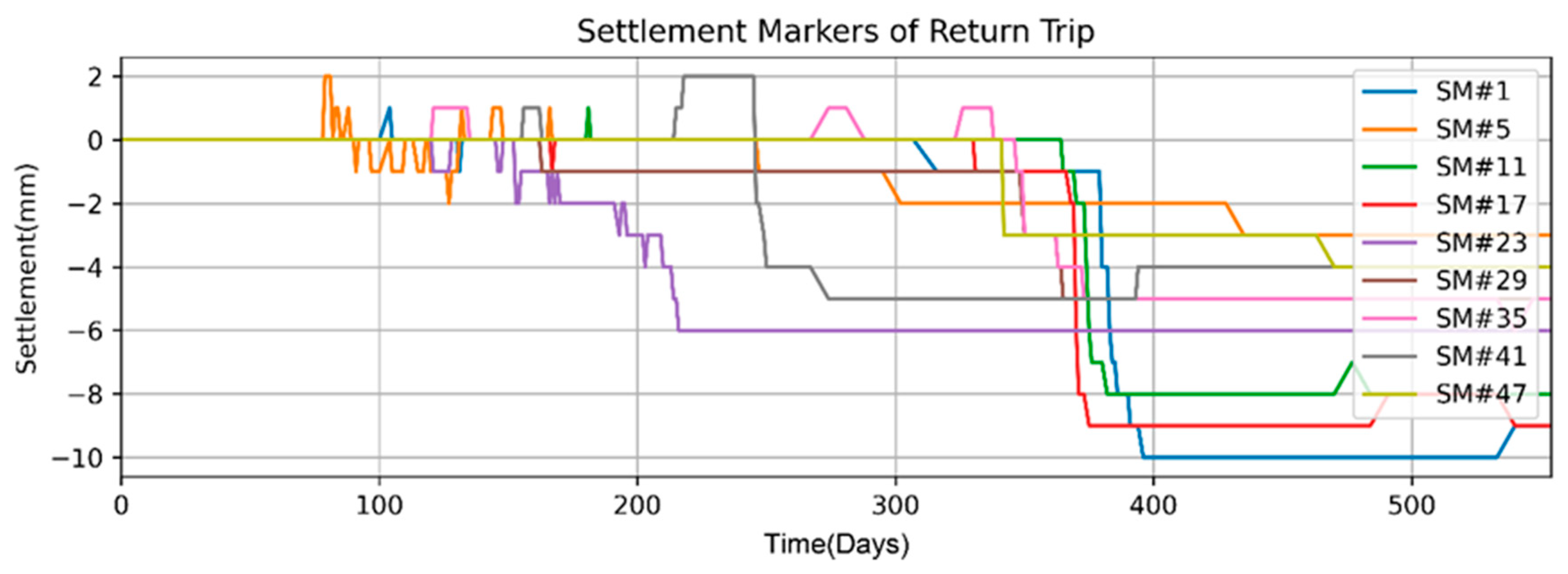
3.3. Occurrence of Subsidence

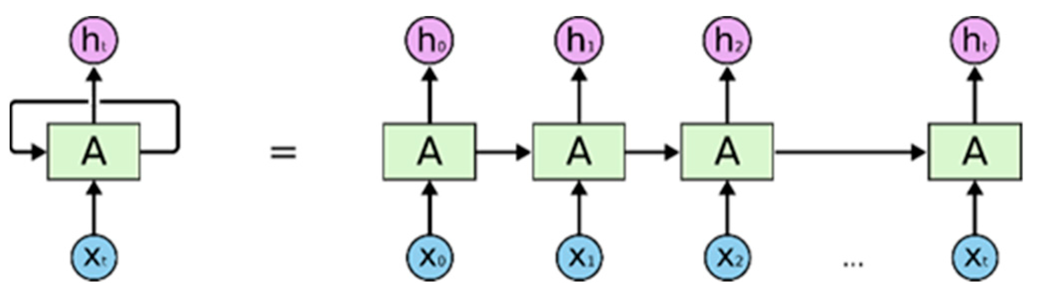
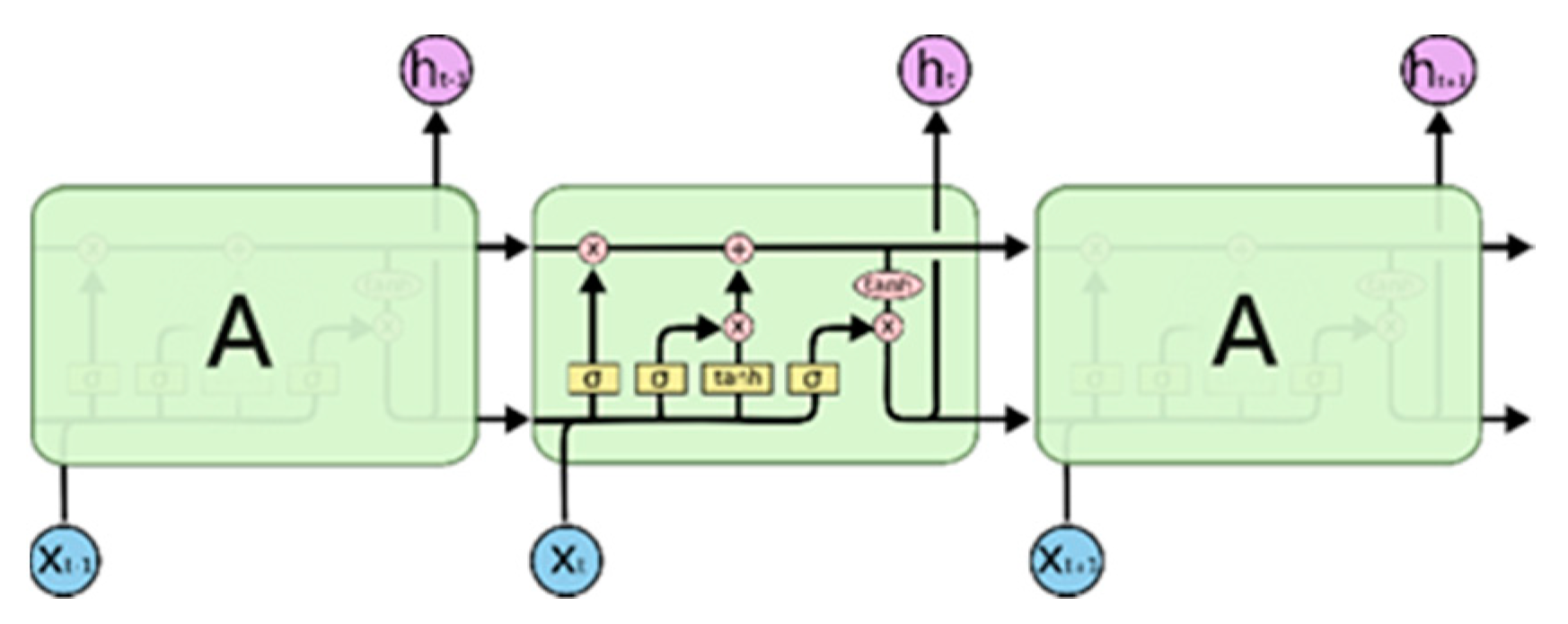
Figure 4 provides the layout of the 48 settlement markers along the alignment. As the tunnel was a single-track twin tunnel, the TBM departed from the launching shaft and reached the arrival shaft along the southern tunnel and then returned to the launching shaft along the northern tunnel. As the TBM head approached, some markers within the influence zone began to record the initiation of movement, as shown in Figure 2. As the TBM head passed through, the settlement rate peaked and then converged onto long-term settlement.

Figure 5 depicts the monitored settlements from the markers installed along the southern tunnel. Marker #2 recorded the earliest occurrence of settlement. The usual trend of settlement consists of an initial heaving followed by a maximum settlement rate within a short time and then gradual convergence on a final value, as shown in markers #2, #7, and #19.

Figure 6 depicts the monitored settlements from the markers installed along the northern tunnel. Markers #1 and #5 recorded the earliest occurrences of settlement. Unlike the trends associated with the markers along the southern tunnel, the northern tunnel showed a long lead between the initial movement and the highest rate of settlement, because the settlements monitored along the southern tunnel were influenced by the tunnel driving along the southern tunnel excavation, with the TBM head returning to the launching shaft after a round trip from the launching shaft.

4. LSTM Networks

The LSTM network, which was proposed by Hochreiter and Schmidhuber (1997), is a special variant of a recurrent neural network (RNN), in which the connections between nodes from a directed graph are depicted along a temporal sequence. Any RNN and its variants have a trained form consisting of repetitive units, as shown in Figure 7. In traditional RNNs, the repetitive unit alone has a simple structure, such as a tanh layer. When dealing with long-term dependency problems, a traditional RNN involves multiple matrix multiplications, which can lead to exploding and/or vanishing gradient problems. To solve such problems, many RNN variants have been developed, such as the echo state network, the gated recurrent unit, and LSTM. Among these variants, LSTM is the most popular as it has the proven capability of solving exploding and vanishing gradient problems.

As an RNN variant, LSTM is connected by repetitive units. However, unlike a traditional RNN, the repetitive units of LSTM are composed of a cell state, an input gate, an output gate, and a forget gate (Figure 8). The cell remembers values over arbitrary time intervals, while the three gates regulate the flow of information into and out of the cell. In the typical LSTM unit depicted in Figure 8, the blue circle represents the network’s input, the yellow boxes represent the learned neural network layers, and the orange shapes represent element-wise operations, such as addition.

The key to LSTM is the cell state (C_t); when it runs straight down the entire chain, only minor interactions occur. Information can easily and simply flow along the chain unaffected and maintain its integrity. The merging arrows represent vector concatenation, while the forking arrows represent vector duplication. The gates in LSTM models are designed to remove or add information to the cell state. They are composed of a sigmoid layer and multiplication operations. The sigmoid layer output is a value between zero and one, which indicates the weight of information flow. An LSTM model achieves control and protection of the cell state through these three gates. The forget gate decides what information will be disposed of from the cell state. This transfer can be defined as:

f_t = σ (W_f · [h_t−1, x_t] + b_f)

(1)

where σ is the sigmoid activation function, W_f is the weight of the connections between neurons, h_t−1 is the output of the last neuron, x_t is the input of the current neuron, and b_f is the bias of the neuron. The forget gate determines the effect of the input on the current cell state, as well as the preservation and discarding of the previous cell state. The input gate determines how much new information will be stored in the current cell state. This transfer can be defined as:

i^t = σ(W_i · [h_t−1, x_t] + b_i)

(2)

C˜_t = tanh(W_C · [h_t−1, x_C] + b_C)

(3)

where tanh is the activation function, and b_i and b_C are the biases of the neural network. The sigmoid layer decides which value will be updated, while the tanh layer creates a new vector C˜, which can be added to the cell state. After completing the above steps, the updated cell state can be defined as:

C_t = f_t ∗ C_t−1 + i_t ∗ C˜_t

(4)

where ∗ is an element-wise production operation. In the updating procedure of the cell’s state, the old cell state C_t−1 is multiplied by ft to forget some information, and the new candidate value i_t ∗ C_t from the input gate is then added. After the cell state has been updated, the output gate will output the current cell state. This transfer can be defined as:

o_t = σ (W_o · [h_t−1, x_t] + b_o)

(5)

h_t = O_t ∗ tanh(C_t)

(6)

In summary, the above three gates are composed of sigmoid and tanh neural network layers, which help in selecting effective information.

5. Training Model and Prediction for Subsidence

5.1. Challenges

The training of machine data and subsidence measurements are carried out in two phases. The first phase trains the machine data and generates input for the second phase. The subsequent phase trains the input from Phase One, which is the weight of the hidden layer of Phase One neural network model, and eventually predicts subsidence.

The machine data from various TBM sensors consisted of more than 700 items. The followings were chosen to serve as the input for Phase One training. Penetration is a key parameter for training as the sequence is organized in such a way that the rest of the parameters support the penetration prediction. The input sequence was a series of chosen records: penetration, chainage, thrust cylinder, torque of cutting wheel, current pressure of real lance one, pressure of excavation chamber one, rotation speed of screw conveyor drive, calculated excavated material depending on advance one, the actual quantity of excavated material belt scale one, and stroke-thrust cylinder.

Machine data were recorded every 10 s over a span of several years while TBM was driving. The amount of machine data from a TBM can be overwhelming, as a human cannot review and interpret it all to derive tangible outcomes, such as the potential risk of subsidence around a job site.

The diversity of methods of operating the machine and the resulting range in construction quality make the problem more complicated. For example, it is relatively easy to infer that subsidence will be correlated with the number of rings installed. However, it is difficult to estimate how closely subsidence will correlate with the skill and experience of a TBM operator. While face pressure should be well managed and controlled, because the balance of the volume of excavation and spoil must be cross-checked repeatedly, it is not so easy in practice to simultaneously supervise all critical elements.

Machine learning in Phase One is an attempt by artificial intelligence to overlook the TBM’s entire advance, and capture the features that may be related to adversarial events. Penetration, revolutions per minute, and chainage may indicate the location and speed of the excavation, chamber pressure, and thrust force may indicate the earth pressure balance, and the actual and calculated excavation volume may indicate the material balance. If the face pressure is well controlled, then subsidence will be minor, and vice versa. We anticipated the output of Phase One would capture the relevant features in this regard.

Machine data were produced at 10 s intervals while subsidence was measured at intervals of every few days to weeks, according to the distance from the excavation face to the settlement marker. For outputs of a single settlement recording, the maximum amount of machine data as input was 95,040 fields, even if only 11 of 700 fields were recorded. To train the machine data and subsidence in a single phase would have required a period of trial-and-error training to produce a useful LSTM model, which is impractical in terms of both training time and computing cost. We split the process into two phases, for training the machine data and identifying critical features associated with subsidence. By training for subsidence with features identified in the previous phase, LSTM models for phases can be obtained successfully with fewer resources.

Ten records of machine data with the above 11 fields were flattened into a column and then fed into the LSTM model, which generated one output prediction, which was then used as the input for the next forward propagation. The loss, which is the mean square root of the difference between the ground-truth penetration and the predicted penetration, was defined, and an Adam optimizer with a learning rate of 0.001 steps was used to minimize errors. We assumed that the machine data encapsulated the overall performance of the TBM and construction quality so that it had a substantial impact on the occurrence of subsidence.

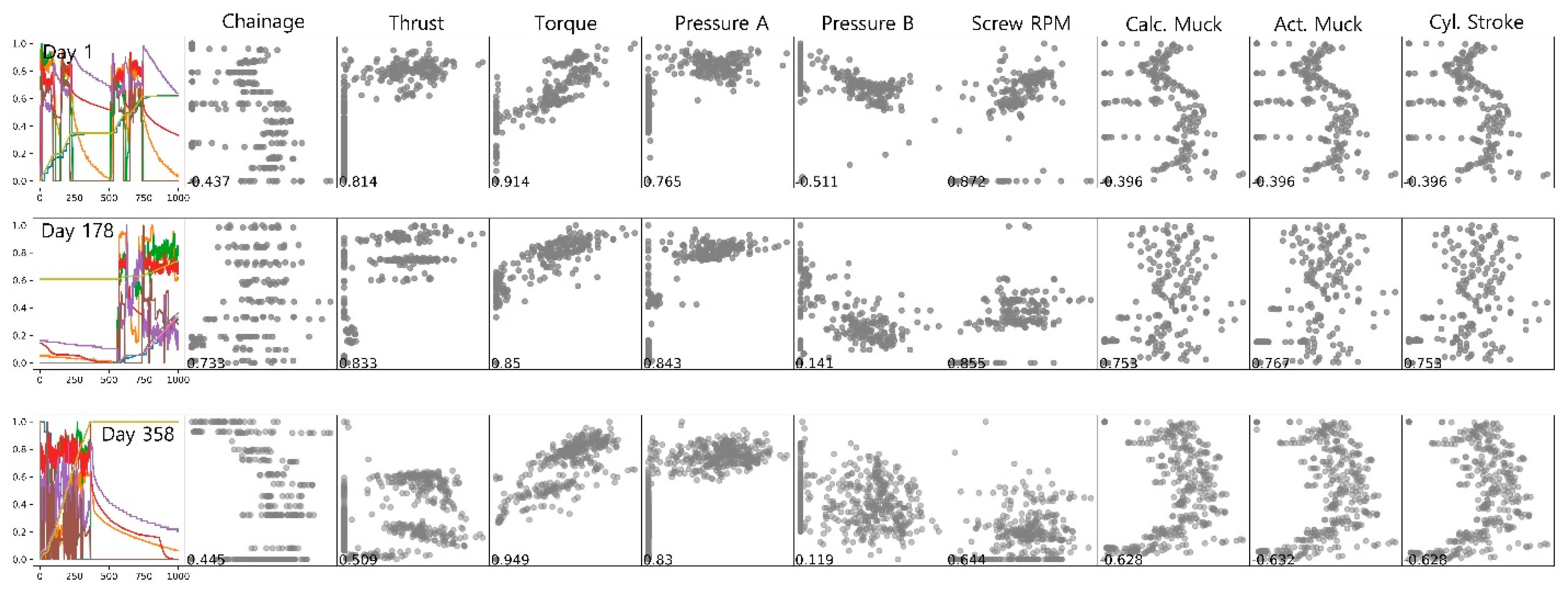
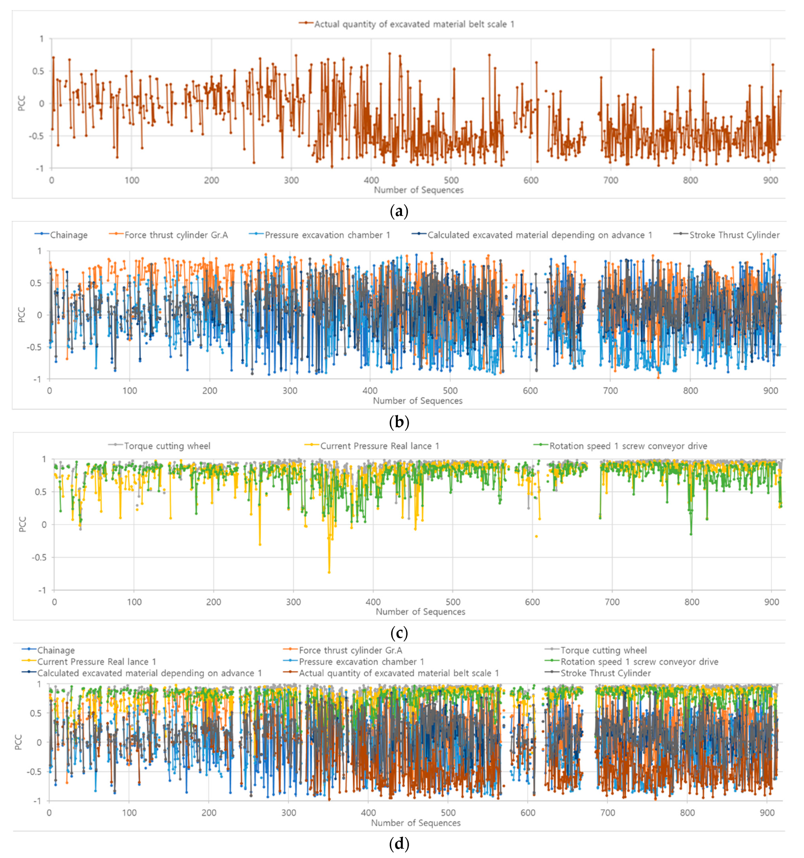
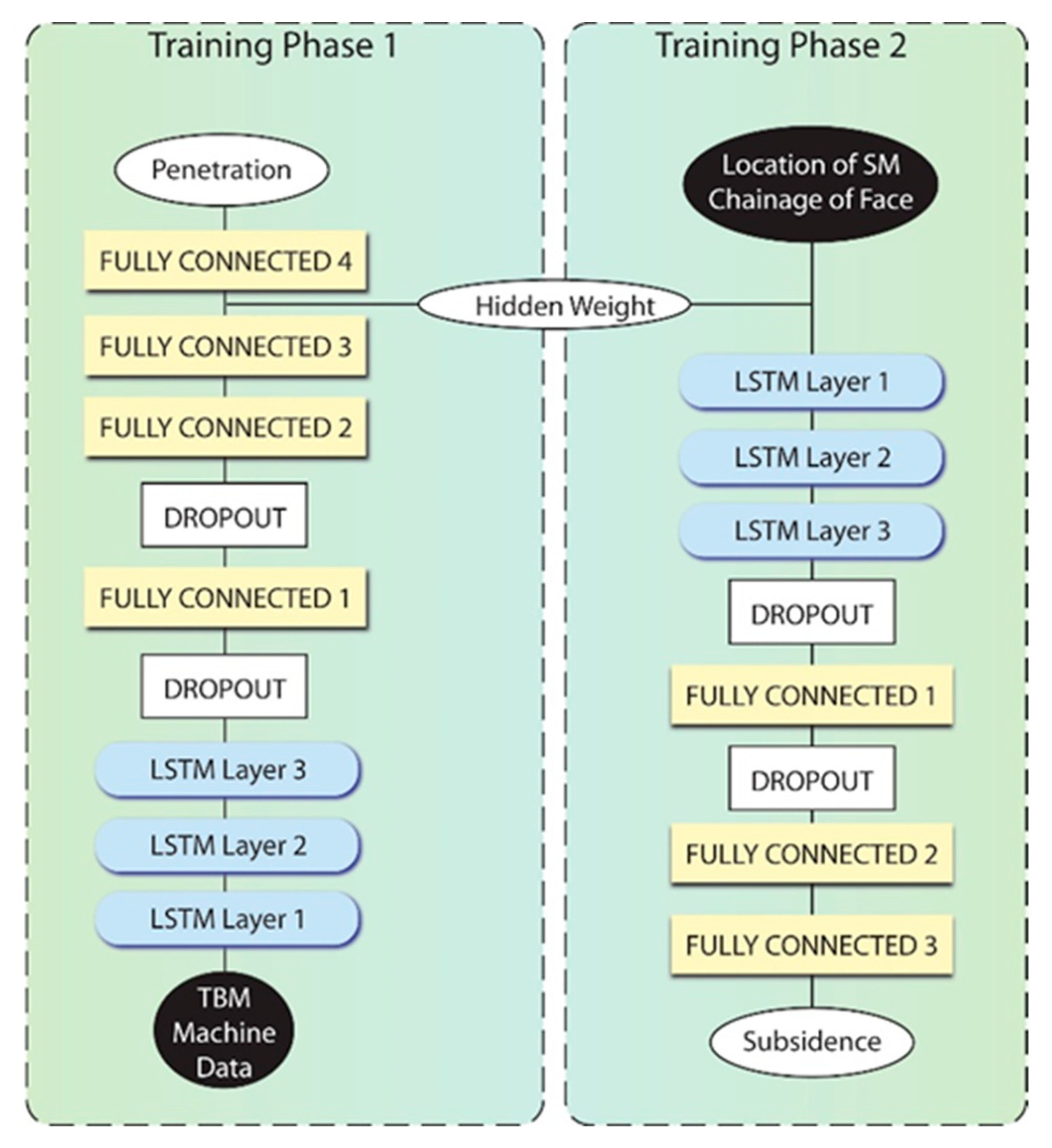
5.2. Training Phase One: Feature Extraction from Machine Data

As discussed in the previous section, we used engineering judgment to select some of the items. Sensitivity analyses of the other items are incomplete and could be served as a subject for future research. Eleven items were chosen in the training phase: penetration, chainage, thrust cylinder (Gr. A), torque cutting wheel, current pressure real lance one, pressure excavation chamber one, rotation speed one screw conveyor drive, calculated excavated material depending on advance one, the actual quantity of excavated material belt scale one, and stroke thrust cylinder.

Data were recorded while the TBM was in operation on each of the approximately 160 working days over the course of a year. Machine data recorded when the TBM was idling were excluded. Because the machine data were recorded about every 10 s, there was a maximum of 8460 records in a day, but the actual number of daily records was fewer due to ring building, cutter-head intervention, equipment breakdown, or maintenance.

The machine data were turned into a sequencing batch comprising 1000 records taken every 10 s, producing a sequence 2.8 h long. A maximum of 500 iterations of training was carried out for each batch. The window size for training a batch was 10, the input size of the model was 1100, which was 11 by 10 flattened, and the output size was one, which represented penetration.

Figure 9 depicts the complicated dynamics taken from the various TBM sensors in response to the driving of the machine. We expected that the machine data from training could be organized into meaningful features, such as the amount of excavation work completed, control of chamber pressure, maintenance of muck balance, and speed of the TBM drive.

In order to analyze the sensitivity of chosen parameters with respect to penetration, the Pearson correlation coefficient (PCC) was used as shown in the Equation (7),

$${\mathrm{r}}_{\mathrm{x},\mathrm{y}}\left({\mathrm{x}}_{\mathrm{i}}\right)=\frac{\mathrm{n}{{\displaystyle \sum }}_{\mathrm{i}=1}^{\mathrm{n}}{\mathrm{x}}_{\mathrm{i}}{\mathrm{y}}_{\mathrm{i}}-{{\displaystyle \sum }}_{\mathrm{i}=1}^{\mathrm{n}}{\mathrm{x}}_{\mathrm{i}}{{\displaystyle \sum }}_{\mathrm{i}=1}^{\mathrm{n}}{\mathrm{y}}_{\mathrm{i}}}{\sqrt{\mathrm{n}{{\displaystyle \sum }}_{\mathrm{i}=1}^{\mathrm{n}}{\mathrm{x}}_{\mathrm{i}}^2-{\left({{\displaystyle \sum }}_{\mathrm{i}=1}^{\mathrm{n}}{\mathrm{x}}_{\mathrm{i}}\right)}^2}\sqrt{\mathrm{n}{{\displaystyle \sum }}_{\mathrm{i}=1}^{\mathrm{n}}{\mathrm{y}}_{\mathrm{i}}^2-{\left({{\displaystyle \sum }}_{\mathrm{i}=1}^{\mathrm{n}}{\mathrm{y}}_{\mathrm{i}}\right)}^2}}$$

(7)

where r_x,_y(x_i) is the PCC of the effect of i-th influential factor on penetration (y_i), x_i is the value of influential factors, and n is the total number of samples.

Figure 10 shows the time series excavation records in the first box and thr PCCs of the chosen parameters against the penetration of TBM driving in the following boxes on days 1, 178 and 358, which were the first, midst, and last stages of the TBM excavation, respectively. From a few cases of PCC analyses, chainage show low Pearson correlation, which are rather dependent than the influential parameters on penetration. Torque, thrust, pressure A (current pressure at real lance one) and screw RPM show mild positive correlation, whereas pressure B (excavation chamber one pressure), the calculated and actual muck volume, and thrust cylinder stroke show a negative correlation. This is in line with the common intuition that driving parameters, such as thrust and torque, are positively influential to penetration, and that ahigh chamber pressure for the support of excavation face is negatively influential, i.e., it maintains a low penetration.

Evolution of the Pearson correlation coefficients with respect to penetration for the entire duration of TBM excavation are shown in Figure 11. Figure 11a–d show negative, neutral, and positive correlation parameters and the combination of all, respectively. Unlike Figure 10, the parameter of negative PCC is the actual quantity of excavated material, which is against the common intuition that a high penetration accompanies the high quantity of excavated muck. However, it is consistent with the common intuition that the parameters of positive PCC are torque, pressure A, and screw RPM, as shown commonly in the Figure 10 and Figure 11. One thing to note is the Pearson coefficients highly fluctuate, such that oversimplification of the machine data, such as average thrust or torque of ring data, may eliminate the critical features related to the characteristics of the machine drive.

Figure 12 shows the graphical representation of hidden features, which are the floating-point numbers, and are turned into grey scale according to their value from zero to one, for black to white, respectively. We reiterate that hidden features are part of the model, which is trained for the prediction of next penetration based on the previous machine parameters, such as thrust, torque, and chamber pressure. Once the model becomes good at predicting the penetration, then one of the hidden layers is exported to represent the way the machine drove for about 2 h.

The Phase One model has three LSTM layers, as well as four layers of fully connected layers. The third and fourth fully connected layers were devoted to extracting and saving the weight of the hidden layers, which had 20 and 10 items, respectively. A dropout rate of 0.001 was used for regularization. During Training Phase One for all records, the weights of the third and fourth hidden layers were saved. Approximately 915,000 machine data fields were condensed into 915 sequences of hidden features.

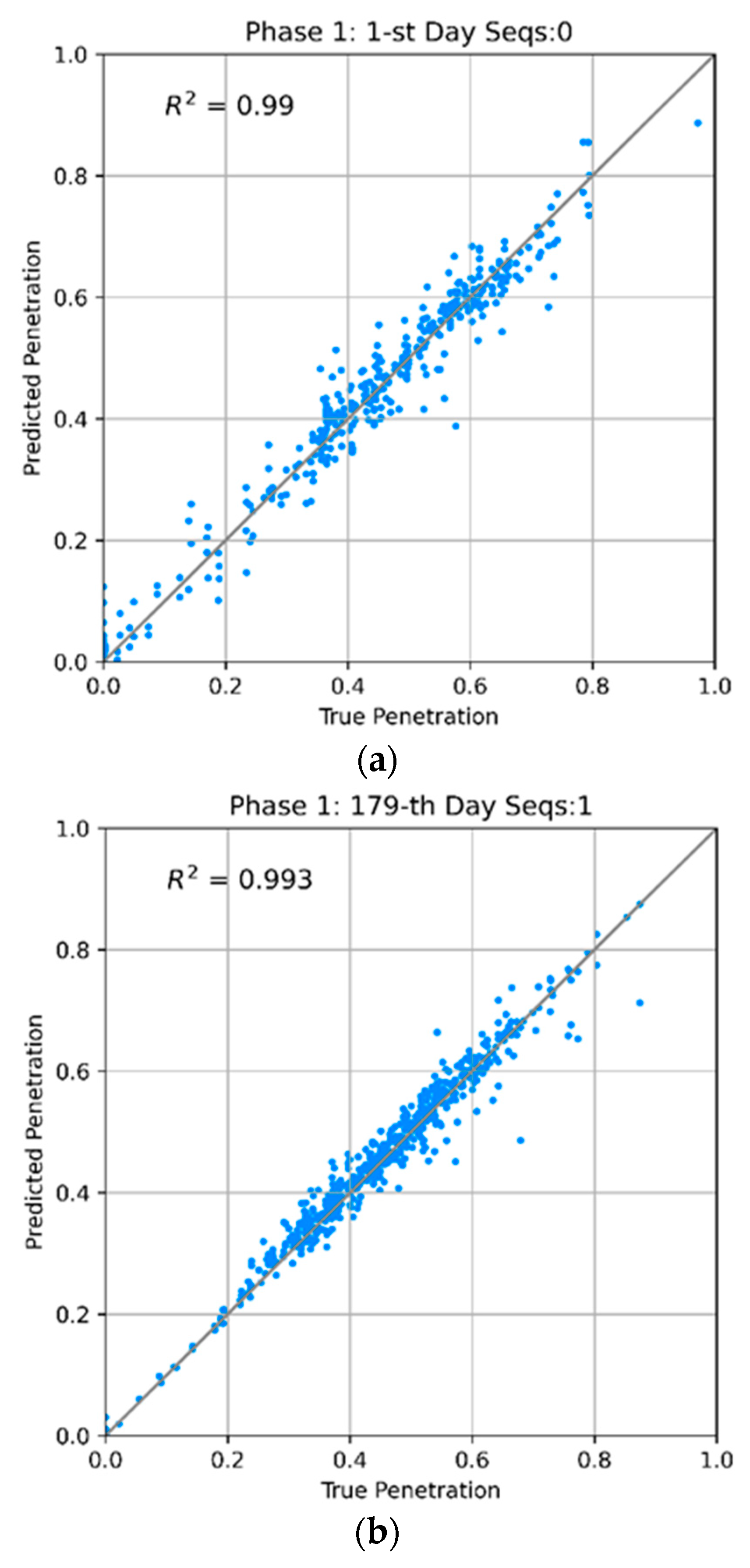
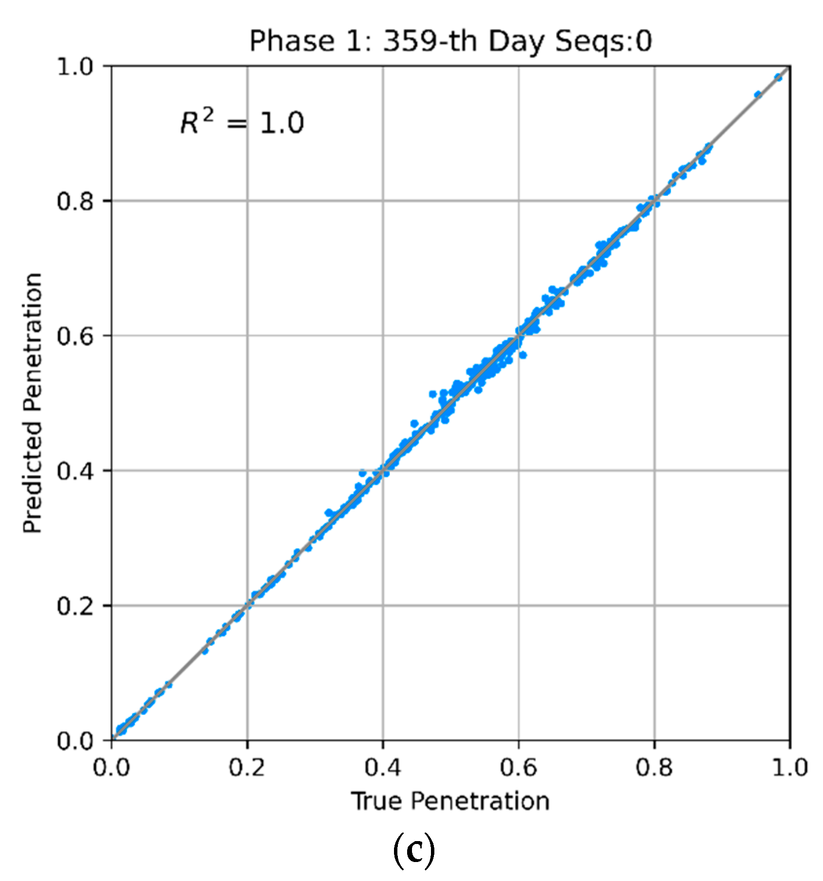
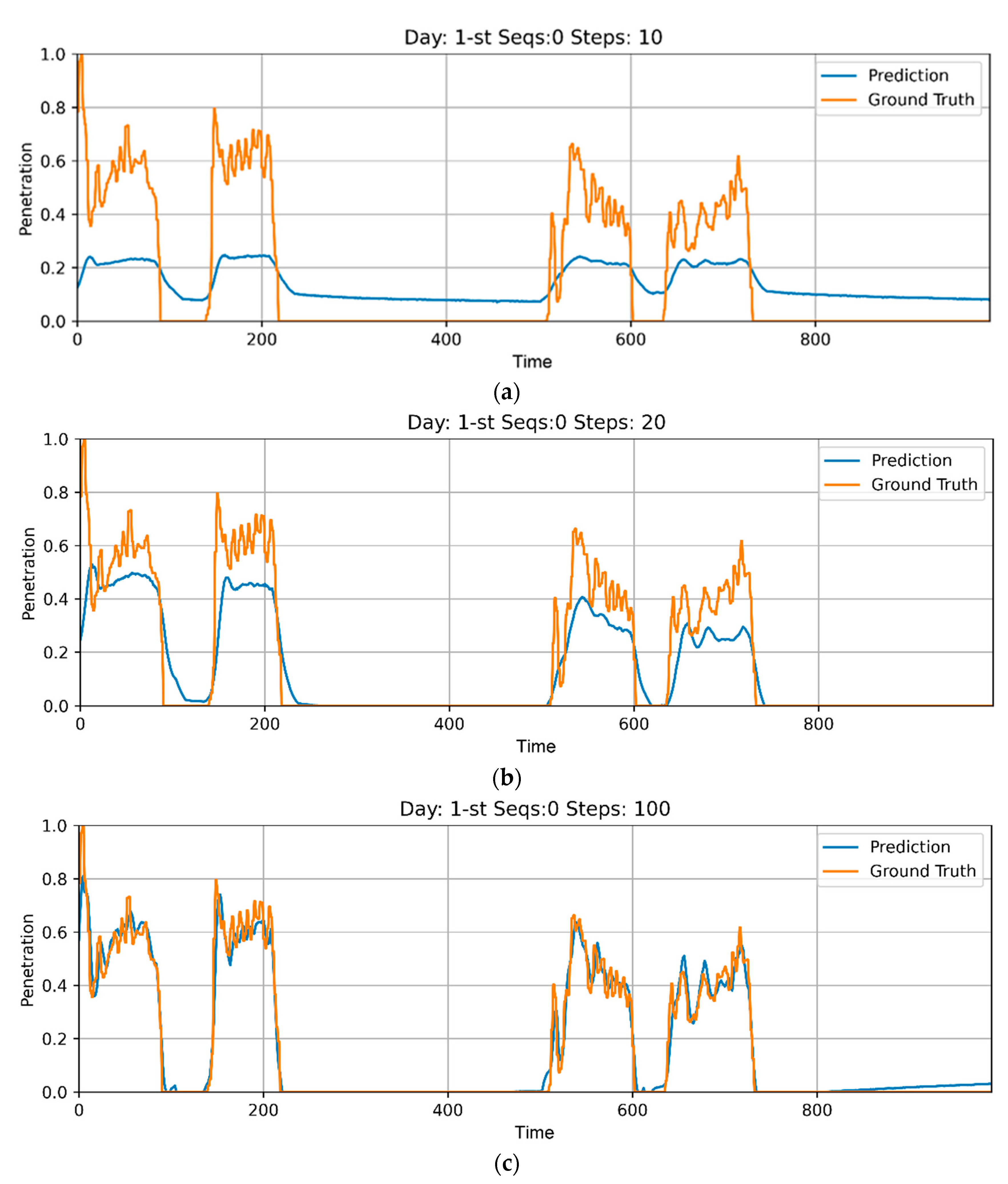
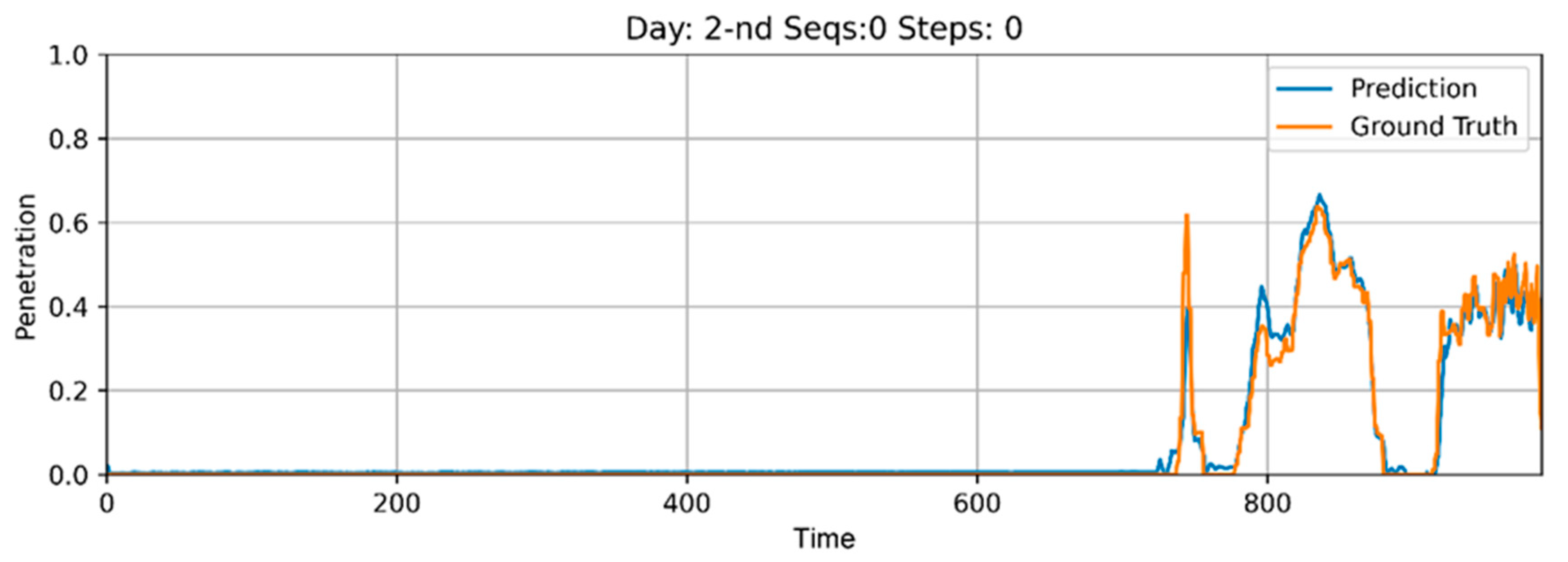
5.3. Results of Phase 1 Training

Figure 13 shows the evolution of the loss, which represents the progress of the machine data learning. The loss at step zero was small because the training process had begun using the pre-trained model file by accident, after multiple attempts to initiate training. However, the performance of the Phase One model was suitable for the generation of an input sequence for Phase One training model.

Figure 14a–c shows the evolution of the prediction versus the ground truth of the machine data for the 500 training iterations. At first there was no capability of prediction, as the initial weights were random. However, after ten iterations, the model began to capture the penetration pattern, and after 100 iterations, the trained prediction sequence closely matched the ground-truth sequence.

Figure 15 shows the evolution of the loss of training for the first batch of the second-day machine data, which represents the progress of the machine data learning process. Similar to Figure 13, the loss at the initial step was even smaller, because the training had just begun using the pre-trained model file from previous learning steps. Periodic jumps of the loss might be due to the dropout layers for the regularization and avoiding overfitting.

Because the purpose of Phase One training was to extract sequences of excavation features to provide input for subsequent Phase Two training, the entire data set was used for training, but not for the evaluation. However, the effectiveness of the evaluation was demonstrated by the fact that the loss on the second-day excavation sequence at the zeroth iteration was already low and the prediction well matched with the actual data from the beginning of training steps, as shown in Figure 16.

Figure 17 shows the prediction performance of the Phase One training model at (a) the first, (b) midst and (c) last day of excavation. It shows a great performance, as the coefficients of determinant (R2) are 0.99, 0.993 and 1.0, respectively, for the first, midst, and last day, which supplemented the good performance shown in the Figure 14 and Figure 16.

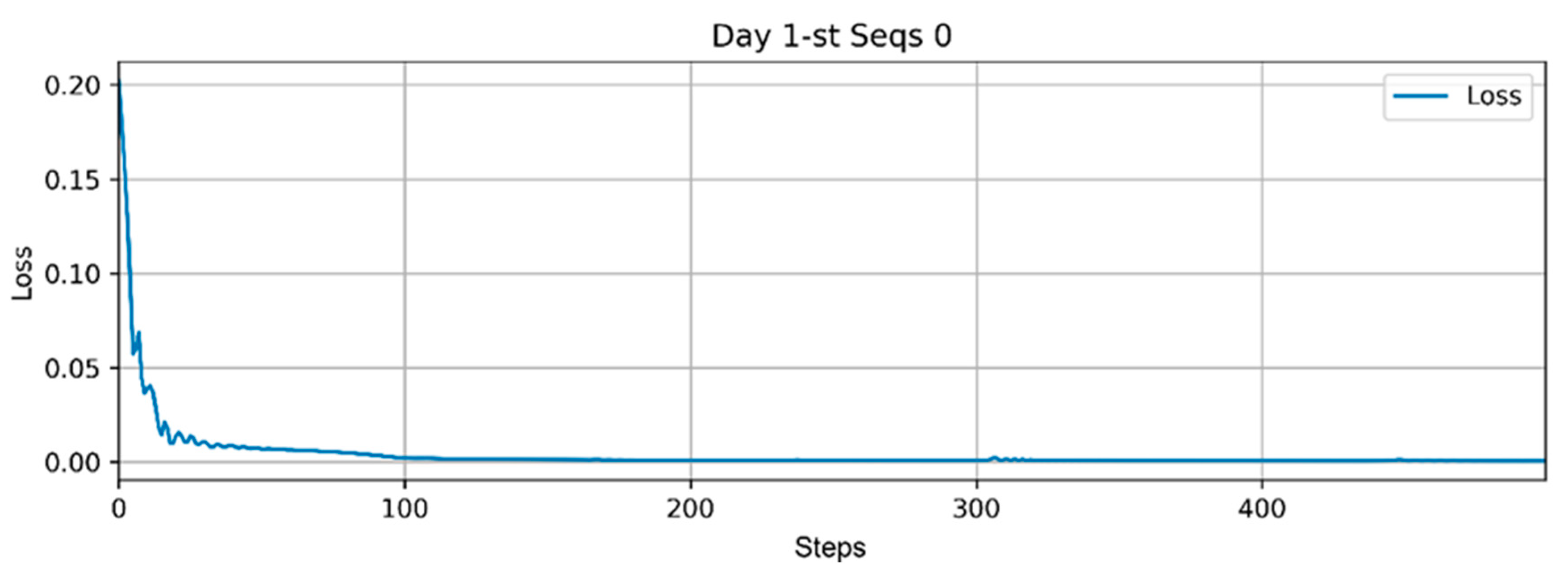
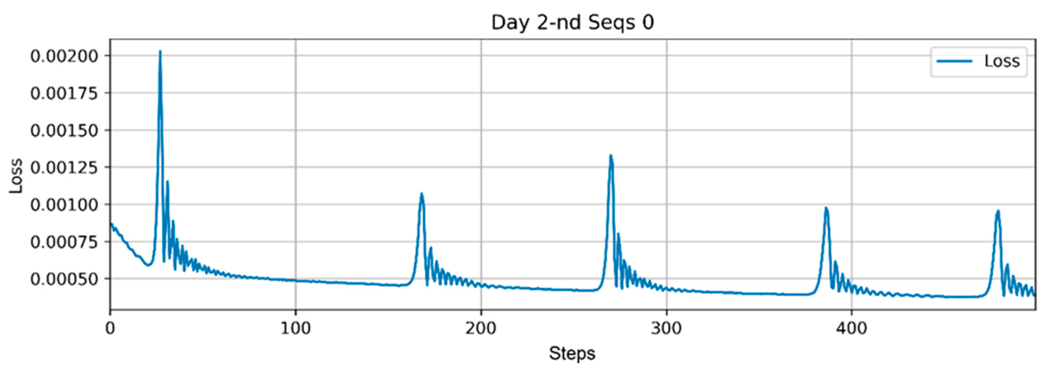
5.4. Training Phase Two: Subsidence Estimation of Features from Machine Data

The purpose of Training Phase Two was to train the weights of the hidden layers and to predict subsidence. Subsidence is governed by how the TBM drives, how well the face pressure is controlled to avoid or minimize ground movement, and the distance of the excavation work. Subsidence will be relatively high if the settlement marker is near the excavation face and the quality of the excavation is poor. However, subsidence will be low if either the excavation quality is high, or if the settlement marker is far from the excavation face. The output from Training Phase One (subsidence monitoring) and the distance of the settlement markers from the excavation face constituted the input for Phase Two model.

The structure of the Phase Two model was essentially identical to that of the Phase One model. If penetration was the key item for training in Phase One, then subsidence was the key item for training in Phase One. In the Phase One model, ten other fields, including chamber pressure, torque, thrust, and muck-out volume, were chosen as supplementary items for training. In the Phase Two model, four other fields, including chainage of excavation face, chainage and offset of settlement markers, and date, were the supplementary items for training. Settlement measurements were made at 48 settlement markers. Measurement data were assigned to the training and test sets, which received data from 44 and 4 markers, respectively. To be successful, the Phase Two model should perform well for the test set.

The Phase Two model has three LSTM layers, as well as three layers of fully connected layers. Similar to the model for Phase One, a dropout rate of 0.001 was used for regularization. As a summary, Figure 18 displays the flow of Phase One and Phase Two NN models.

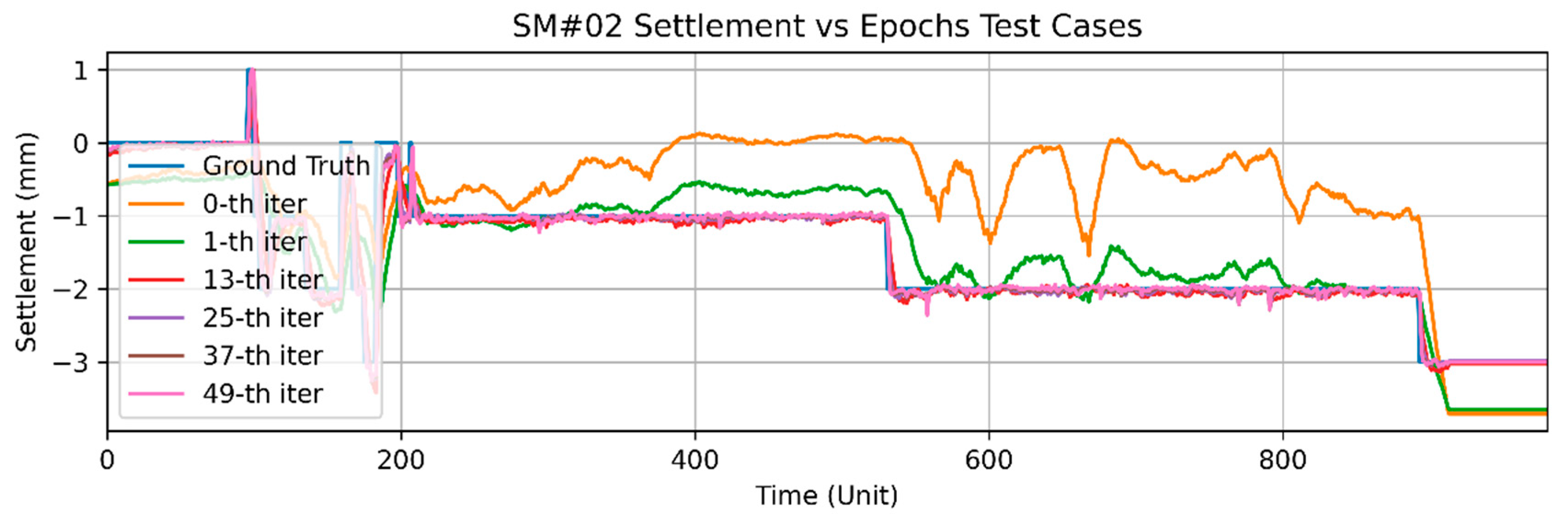
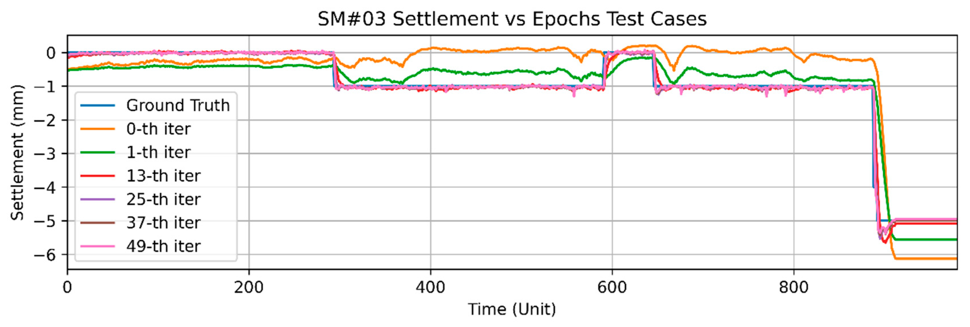
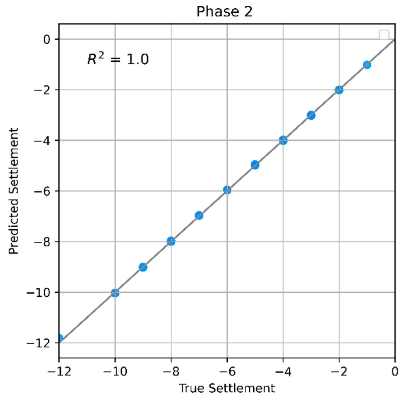
5.5. Results of Phase Two Training

As shown in Figure 19, the loss of the test and training sets rapidly decreased to a negligible level. At the beginning of Phase Two training, the loss of the test set was lower than that of the training set, but the loss in the test sets became stagnant, while that of the training set steadily decreased. In the end, the losses in both the training and test sets converged to negligible levels.

Figure 20 shows the prediction performance of the Phase Two model. It shows a great performance, whose coefficient of determinant (R²) is 1.0. As the actual settlements are measured with the precision of millimeters, points of actual and predicted settlements in truth-prediction plot are discrete in mm-wise integer numbers.

Figure 21 illustrates the evolution of predictions for the ground truth for one of the training sets. At the first epoch of training, the prediction of the training set roughly followed a timing of the occurrence of subsidence. At the thirteenth epoch, the prediction was relatively consistent in terms of the timing and maximum value of the settlement. At the final (49th) epoch, the prediction and ground truth were closely matched, with only subtle fluctuations in settlement within a brief period. While this may have been a result of overfitting, Figure 22 and Figure 23 show the satisfactory performance of the LSTM model in Phase Two: the evolution of the prediction of the test sets, which were not made for training, were similar or even superior to, those of the training set with respect to ground truth.

The superior performance of the Phase Two model for the test sets demonstrated that the weights of the hidden layer of the Phase One model were appropriate features for the training of settlement monitoring records, suggesting that this approach could be successfully applied to current construction projects.

5.6. Discussion

The input sequence for Phase 1 training was a series of chosen TBM data: penetration, chainage, thrust cylinder, torque of cutting wheel, current pressure of real lance, pressure of excavation chamber, rotation speed of screw conveyor drive, calculated excavated material depending on advance, the actual quantity of excavated material belt scale and stroke-thrust cylinder. Among parameters, penetration is a key parameter for training in such a way that the rest of the parameters are supporting the penetration prediction. The output from Training Phase one, subsidence monitoring and the distance of the settlement markers from the excavation face constitute the input for Phase two model.

The choice of the machine data as an input for training is not by sensitivity analysis but by engineering judgement of authors. It was by far more successful than initially anticipated as shown in Figure 19 and Figure 20, in which LSTM approach can be effectively applied to predict the ground surface settlement. However, a very long computation time was required for LSTM model training of phase 1 due to the large amount of the input data.

Therefore, next step would be performing the sensitivity analysis to optimize the number of parameters for phase one and applying various AI models to predict the risks of excessive subsidence or sinkhole induced by TBM excavation in mixed ground condition. It would be a meaningful to investigate the performance of the AI models for the prediction of ground subsidence as well as the machine parameters of the TBM.

6. Conclusions

Due to the high demand for new transportation infrastructure, large numbers of tunnels and underground spaces are being constructed for urban roads, railways, and electrical and telecommunication infrastructures, which are associated with rapid urbanization. Among the risks posed by tunnel construction in a congested urban area are the risks of subsidence or the creation of a sinkhole. The resulting costs to society from such incidents can be significant. Tunneling using a TBM, which can apply face pressure to stabilize the ground, is widely used to address the threat of subsidence. However, to effectively prevent such incidents, it is crucial to be able to predict where they might happen, so that it enables the engineer to plan beforehand.

It is well recognized that subsidence during tunnel construction is closely correlated with the driving characteristics of the TBM. However, so far, the use of complete sequences of machine data is unprecedented for capturing the features that correlates the way that TBM drives with resulting settlement. A TBM generates data from various machine sensors, including thrust, torque, chamber pressure, and muck discharge volume, which would contain the TBM driving characteristics including the response of ground against the thrust force of the boring machine.

Throughout this study, it was shown that machine data could encapsulate the features related to settlement occurrence patterns. The cause and consequence, i.e., TBM driving and settlement, can be modeled with an LSTM and fully connected layers separately. Data can be obtained from the TBM every 10 s, whereas settlement is recorded daily or weekly, according to the distance of the excavation face. The Phase One model for TBM driving, which is the cause of settlement, can train the TBM data and extract features related to the consequences. The output of Phase One model is the weights of the hidden layers, which are extracted features from machine data, and which formed the input for the Phase Two model, together with additional information, such as the location of the settlement markers, and tunnel face and settlement records.

The performance of the models for the test sets demonstrates that the weights of the hidden layer of Phase One model are appropriate for the training of settlement-monitoring records and, suggests that this two-phase LSTM approach can be effectively applied to TBM excavation projects.

References

1. Ko, T.Y.; Lee, S.W. Effect of Rock Abrasiveness on Wear of Shield Tunneling in Bukit Timah Granite. Appl. Sci. 2020, 10, 3231. [Google Scholar] [CrossRef]
2. Peck, R. Deep excavations and tunneling in soft ground. In Proceedings of the 7th International Conference on Soil Mechanics and Foundation Engineering, Mexico City, Mexico, 29 August 1969; pp. 225–292. [Google Scholar]
3. You, K.H.; Jung, S.T. A study on the behavior of surface settlement due to the excavation of twin TBM tunnels in the clay grounds. J. Korean Geo-Environ. Soc. 2019, 20, 29–40. [Google Scholar] [CrossRef]
4. Kasper, T.; Meschke, G. On the influence of face pressure, grouting pressure and TBM design in soft ground tunneling. Tun-Nelling Undergr. Space Technol. 2006, 21, 160–171. [Google Scholar] [CrossRef]
5. Zhang, K.; Lyu, H.M.; Shen, S.L.; Zhou, A.; Yin, Z.Y. Evolutionary hybrid neural network approach to predict shield tunneling induced ground settlements. Tunn. Undergr. Space Technol. 2020, 106, 103594. [Google Scholar] [CrossRef]
6. Mair, R.; Taylor, R.; Burland, J. Prediction of ground movements and assessment of risk of building damage due to bored tunneling. In Geotechnical Aspects of Underground Construction in Soft Ground; Balkema, Brookfield: Rotterdam, The Netherlands, 1996; pp. 713–718. [Google Scholar]
7. Vorster, T.E.B.; Klar, A.; Soga, K.; Mair, R.J. Estimating the effects of tunneling on existing pipelines. J. Geotech. Geo-Environ. Eng. 2005, 131, 1399–1410. [Google Scholar] [CrossRef]
8. Franza, A.; Marshall, A.M. Empirical and semi-analytical methods for evaluating tunneling-induced ground movements in sands. Tunn. Undergr. Space Technol. 2019, 88, 47–62. [Google Scholar] [CrossRef]
9. Meschke, G. From advance exploration to real time steering of TBMs: A review on pertinent research in the collaborative research center, “interaction modeling in mechanized tunneling”. Undergr. Space 2018, 3, 1–20. [Google Scholar] [CrossRef]
10. Lee, H.; Choi, H.; Choi, S.; Chang, S.; Kang, T.; Lee, C. Numerical Simulation of EPB Shield Tunneling with TBM Operational Condition Control Using Coupled DEM–FDM. Appl. Sci. 2021, 11, 2551. [Google Scholar] [CrossRef]
11. Chou, J.S.; Lin, C. Predicting disputes in public-private partnership projects: Classification and ensemble models. J. Comput. Civ. Eng. 2013, 27, 51–60. [Google Scholar] [CrossRef]
12. Bouayad, D.; Emeriault, F. Modeling the relationship between ground surface settlements induced by shield tunneling and the operational and geological parameters based on the hybrid PCA/ANFIS method. Tunn. Undergr. Space Technol. 2017, 68, 142–152. [Google Scholar] [CrossRef]
13. Chen, R.; Zhang, P.; Wu, H.; Wang, Z.; Zhong, Z. Prediction of shield tunneling-induced ground settlement using machine learning techniques. Front. Struct. Civ. Eng. 2019, 13, 1363–1378. [Google Scholar] [CrossRef]
14. Kim, C.; Bae, G.; Hong, C.; Park, S.; Moon, H.; Shin, H. Neural network-based prediction of ground surface settlements due to tunneling. Comput. Geotech. 2001, 28, 517–547. [Google Scholar] [CrossRef]
15. Suwansawat, S.; Einstein, H. Artificial neural networks for predicting the maximum surface settlement caused by EPB shield tunneling. Tunn. Undergr. Space Technol. 2006, 21, 133–150. [Google Scholar] [CrossRef]
16. Hasanipanah, M.; Noorian-Bidgoli, M.; Jahed Armaghani, D.; Khamesi, H. Feasibility of PSO-ANN model for predicting surface settlement caused by tunneling. Eng. Comput. 2016, 32, 705–715. [Google Scholar] [CrossRef]
17. Samui, P.; Sitharam, T. Least-square support vector machine applied to settlement of shallow foundations on cohesionless soils. Int. J. Numer. Anal. Meth. Geomech. 2008, 32, 2033–2043. [Google Scholar] [CrossRef]
18. Choi, Y.-H.; Lee, S.S. Predictive Modelling for Blasting-Induced Vibrations from Open-Pit Excavations. Appl. Sci. 2021, 11, 7487. [Google Scholar] [CrossRef]
19. Dindarloo, S.; Siami-Irdemoosa, E. Maximum surface settlement-based classification of shallow tunnels in soft ground. Tunn. Undergr. Space Technol. 2015, 49, 320–327. [Google Scholar] [CrossRef]
20. Santos, O.J.J.; Celestino, T.B. Artificial neural networks analysis of Sao Paulo subway tunnel settlement data. Tunn. Undergr. Space Technol. 2008, 23, 481–491. [Google Scholar] [CrossRef]
21. Shi, J.; Ortigao, J.A.R.; Bai, J. Modular neural networks for predicting settlements during tunneling. J. Geotech. Geo-Environ. Eng. 1998, 389–395. [Google Scholar] [CrossRef]
22. Gao, M.; Zhang, N.; Shen, S.; Zhou, A. Real-time dynamic earth pressure regulation model for shield tunneling by integrating GRU deep learning method with GA optimization. IEEE Access 2020, 8, 64310–64323. [Google Scholar] [CrossRef]
23. Kim, Y.K.; Lee, S.W. Study on Risk Assessment of Mine Subsidence by Machine Learning. Appl. Sci. 2020, 9, 1302. [Google Scholar] [CrossRef] [Green Version]
Figure 1. A traverse settlement trough (Peck, 1969).
Applsci 11 12130 g001
Figure 2. Five phases of settlement according to TBM construction.
Applsci 11 12130 g002
Figure 3. Geological layout along the alignment.
Applsci 11 12130 g003
Figure 4. Layout of settlement markers along the alignment.
Applsci 11 12130 g004
Figure 5. Evolution of settlement markers of a departure trip.
Applsci 11 12130 g005
Figure 6. Evolution of settlement markers of a return trip.
Applsci 11 12130 g006
Figure 7. A recurrent neural network and its unfolding form.
Applsci 11 12130 g007
Figure 8. A long short-term memory neural network.
Applsci 11 12130 g008
Figure 9. Sequence of chosen items of TBM data for machine learning. network.
Applsci 11 12130 g009
Figure 10. Pearson correlation coefficients of parameters with respect to penetration at the first, midst, and last stages of TBM drive.
Applsci 11 12130 g010
Figure 11. Evolution of the Pearson correlation coefficients with respect to penetration. They are listed as: (a) Negative PCC parameter; (b) Neutral PCC parameters; (c) Positive PCC parameters; (d) All parameters combined.
Applsci 11 12130 g011
Figure 12. Features extracted from the hidden layers of LSTM model 1.
Applsci 11 12130 g012
Figure 13. Evolution of the loss of training for the first batch of the first day of machine data.
Applsci 11 12130 g013
Figure 14. Evolution of the trained sequences according to training steps. (a) step 10; (b) step 20; (c) step 100.
Applsci 11 12130 g014
Figure 15. Evolution of the loss of training for the first batch of the second-day machine data.
Applsci 11 12130 g015
Figure 16. Prediction vs. ground truth for the second day at the 0th iteration.
Applsci 11 12130 g016
Figure 17. Prediction performance of the Phase One model. (a) Prediction of penetration on the 1st day; (b) Prediction of penetration on 179th day; (c) Prediction of penetration on the last day.
Applsci 11 12130 g017aApplsci 11 12130 g017b
Figure 18. Phases of machine data and subsidence training.
Applsci 11 12130 g018
Figure 19. Evolution of loss in the training and test sets.
Applsci 11 12130 g019
Figure 20. Performance of settlement prediction.
Applsci 11 12130 g020
Figure 21. Evolution of the trained sequences of settlement (SM#8).
Applsci 11 12130 g021
Figure 22. Evolution of the trained sequences of settlement (SM#2).
Applsci 11 12130 g022
Figure 23. Evolution of the trained sequences of settlement (SM#3).
Applsci 11 12130 g023