1. Introduction
Learning to recognize new objects may be a simple task for humans (even for small children), but successful implementations of this in machines prove to be very difficult. While the challenge of teaching machines how to distinguish (i.e., classify) between a set of pre-learned objects has already seen many solutions which present impressive results, e.g., ResNet50 [
1], the challenge of teaching the same machine on the fly how to learn to classify new objects on top of those already known remains very much unsolved [
2].
In this context, artificial neural networks (NN) have been extensively researched and proven to function with outstanding levels of precision over a variety of applications. The go-to approaches for the first part of the problem (teaching a machine to classify an initial set of objects) are typically based on the application of deep neural networks (DNN). So, intuitively, the solution for the next part of the problem (teaching a machine new objects on the fly) is to elaborate on the existing solutions, but the problem with this is that the trained weights in neural networks are extremely fragile, meaning that any change to accommodate new objects can severely damage their capacity to perform the functions they were trained for. This phenomenon is known as catastrophic forgetting (CF) [
3].
The usual approach for avoiding the problems associated with the addition of new classes (objects) (i.e., avoiding catastrophic forgetting) is to simply retrain the entire network from scratch, using data from all the classes that are intended for the network to be able to classify. The issue with this is that the training process tends to be very computationally heavy and, therefore, time-consuming, even when performed on powerful machines. This may not be a problem in some situations, but it is a problem if the goal is to consistently add new classes regularly. Given that when using currently accessible hardware, the training process often takes between hours and days, it is, therefore, impossible to expect networks to learn multiple classes per day with this approach. This type of learning problem, learning a new class without retraining the entire network, is known as continual learning (CL) [
4], where several other names are also commonly used, such as sequential learning [
5], lifelong learning [
3] and incremental learning [
6]. For a comprehensive explanation about this subject, see [
7].
This paper presents a new continual learning architecture for object classification, the modular dynamic neural network (MDNN), with the intention of creating a framework capable of learning new classes (on the fly) without forgetting the previously learned ones. As already mentioned, the current state of the art (see next section) shows that the methods most effectively used for object classification are DNN based. The presented framework is also DNN based and is divided into two main components: (a) the ResNet50-based [
1] feature extraction component; and (b) the modular dynamic classification component, which consists of multiple sub-networks structured in such a way that they can function independently from one another. In more detail, it consists primarily of a static feature extraction component that passes extracted image features onto a modular dynamic classification component. The modular dynamic classification component is made up of multiple neural networks that serve as binary classifiers which are joined together to form a tree-like structure, where internal classifications dictate the path to follow down the tree of networks. The modules function independently of one another, which means the structure can be dynamic and that, after initializing with at least two classes, new modules can be added as more classes are learned to avoid affecting other modules. Another important advantage of the implemented structure is that classifications can be made using only a percentage of the modules, meaning that the addition of new modules will not have the same negative impact on scalability as it would if every new module had to be processed for every classification. While the scalability of the presented framework has not yet been proven on large datasets, the use of a percentage of the network is undoubtedly lighter in terms of computational requirements compared to the use of the entire network.
The main contribution of this paper is a framework that can learn new classes without having to retrain its entire network of classifiers, with features that help it to cope with the scalability problems that generally come with this type of expanding architecture. The presented framework is in itself original, as the methodology behind its architecture does not directly fit into any of the categories normally used to define CL methods, such as regularization, memory/replay, architecture or parameter-isolation-based methods [
3,
8], where it is, in fact, a kind of mixture of the mentioned categories. It is partially regularization-based because parts of the network are selectively not interfered with while training; partially memory/replay based because some data are stored and re-used; partially architecture-based because the network of modules does expand over time; and partially parameter isolation-based because specific parts of the network are assigned specific tasks. On top of being original in itself, the presented framework possesses a feature that is of particular interest in terms of innovation, which is the modular dynamic training component that is the main reason it is able to learn continuously, as modules can be added over time which are responsible for recognizing classes or groups of classes, and the assignment of which classes are attributed to which modules is done automatically as the network grows progressively.
The test results on the CORe50 dataset [
9] show state-of-the-art results when compared with other CL architectures and, in some cases, the MDNN was even able to almost match results obtained on the same data without CL restrictions (i.e., the final accuracy after learning classes incrementally was similar to that of another network presented with all the data at once). The tests made primarily evaluate the framework’s ability to learn classes incrementally and to re-evaluate its accuracy on old classes as new ones are added to make sure they were not forgotten.
The present section introduced the context and goals.
Section 2 includes the related work on continual learning along with some background concepts.
Section 3 addresses the presented architecture,
Section 4 shows the tests and results of the implemented CL architecture and, finally, the conclusions and future work are presented in
Section 5.
2. Related Work
Neural networks are currently receiving a large amount of interest and are being applied to a large variety of real-world problems. They are currently the go-to choice for image detection, image recognition and the classification of persons, objects or scenes. While they are widely used and considered to be very effective, if the goal is to add new classes to the previously learned ones, and therefore continue the learning process from where they left off, they fail. This is because after learning new classes on the fly, the network’s ability to recognize the previously known classes would be severely reduced; this phenomenon is known as catastrophic forgetting [
3] (as already mentioned in the Introduction).
In this context, continual learning [
4] means being able to update the prediction model for new tasks while still being able to reuse and retain knowledge from previous tasks. CL challenges assume an incremental setting, where tasks are received one at a time and, in addition, most studies on the matter also consider the non-storage of data to be an essential characteristic of a continual learner. Usually, continual learning studies refer to humans as ideal examples of continual learners, examples can be seen in [
2,
3,
5,
8]. This is because, as is the case with NN, a large part of the ideas behind CL are inspired by how researchers presume human brains work, including how the process of consolidation and reconsolidation from short- to long-term memory can occur [
10].
Lesort et al. [
11] presented possible learning strategies, opportunities and challenges for CL, but one of the major problems when dealing with developing CL architectures is the lack of datasets available to test them with. There is a huge amount of datasets to test regular object classification (popular examples include ImageNet [
12] and CIFAR [
13]), but none of them has the fundamental characteristics to test CL, such as rules dictating how many classes should be learned at a time, if new data from known classes should be presented later, and how frequently they should be tested. Lomonaco and Maltoni [
9] proposed CORe50, a dataset and benchmark that is more suitable for testing CL methods when compared with the “usually” used image datasets for object classification. CORe50 takes a variety of factors into account, such as intermediate testing, the order of image capture, different levels of occlusion and illumination, the number of classes to be learned at a time and the use or non-use of new data for previously known classes. The same authors presented a leaderboard (CORe50 benchmark:
https://bit.ly/3klHhhK, accessed on 15 October 2021), where they keep track of both published and unpublished results achieved on the CORe50 benchmark so that they can be easily compared with other CL strategies; however, these results are not necessarily up to date. She et al. [
2] tested a variety of continual learning methods on this dataset in order to evaluate their performance in real-world environments and concluded that the currently employed algorithms are still far from ready to face such complex problems.
Maltoni and Lomonaco [
14] proposed AR1, a CL approach combining architectural and regularization strategies, where they were able to sequentially train complex models such as CaffeNet and GoogLeNet by limiting the detrimental effects of catastrophic forgetting. The reported results on CORe50 [
9] and CIFAR-100 [
13] showed that AR1 was able to outperform other models such as elastic weight consolidation (EWC) [
15], learning without forgetting (LwF) [
16] and synaptic intelligence (SI) [
17].
Additionally, Delange et al. [
8] studied a variety of CL methods and proposed a taxonomy, where they categorized 29 different methods. They came to the conclusion that iCaRL [
18] had the best performance for replay-based methods, MAS [
5] had the best performance for regularization-based methods, and PackNet [
19] had the best performance for parameter isolation methods. However, each method had its own advantages and limitations, e.g., PackNet demonstrated the best accuracy, but even though it can learn a large number of tasks, there is a limit based on the size of the model. For more details about each method please see [
8]. It is also important to mention the approach by Requeima et al. [
20], which consists of a multi-task classification that uses conditional neural adaptive processes; while it might not be directly considered a CL method, it can be applied in CL settings.
van de Ven and Tolias [
21] applied an array of CL methods to three different CL scenarios with increasing difficulties in order to compare their performance in different situations. In the first scenario, each model is aware of the identity of the task being performed, meaning that they can opt to use the best-suited components for the given task. In the second scenario, the task’s identity is no longer known, but the models are only expected to solve the task and not necessarily identify its nature. In the third scenario, the model must be capable of not only solving a given task, but also identifying it.
Parisi et al. [
3] explored three different continual learning approaches (they referred to it as lifelong learning). The first approach is based on the retraining of the entire network using regularization, meaning that catastrophic forgetting is dealt with by having constraints applied to the training of the neural network’s weights. The second approach trains specific sections of the network and expands when necessary, operating as a kind of dynamic architecture, adding new neurons which are dedicated to newly learned information. The third approach is made up of methods that model complementary learning systems for memory consolidation, where they make a distinction between memorizing and learning.
Pellegrini et al. [
22] presented latent replay for real-time CL. The authors make a separation between low-level feature extraction and high-level feature extraction. They also control the rate at which each level is trained so that, when training on new information, the low-level feature extraction is modified only slightly or not at all. This strategy enables them to store intermediate data to be re-used alongside new data when new classes are being learned, avoiding the need to re-perform the low-level feature extraction on the stored data. Very recently, from 2021, two CL surveys were made available [
8,
23] that present overviews of this subject.
To summarize, while there may be references to CL as far back as the 1990s, where ideas and concepts are discussed, almost all the research with practical tests and applications is very recent. The fact that a large number of the research papers employ different terms for CL, and the fact that standardized categories are absent for CL methods or consistent descriptions of CL are indications of just how “new” this area of study is when it comes to practical applications. The state of the art shows, especially in recent studies, that there are various CL approaches with a lot of differences between them. They vary so much that it is hard to find a scenario where they could all be tested equally. Nevertheless, some of the mentioned papers share similarities with the proposed architecture, and those are discussed throughout the paper.
3. Modular Dynamic Neural Network
Throughout the literature, the main goals for building CL architectures are very similar: to solve the catastrophic forgetting problem while at the same time reducing memory consumption and allowing for scalability. In the present framework, those goals are considered to be of great importance, but for a CL method to be functional and applicable to real-world problems, avoiding catastrophic forgetting is considered to be the most important objective to follow (the same happens in the majority of the papers that deal with CL). With the elimination of catastrophic forgetting being the main focus (and to consider memory and network size constraints as secondary goals), the presented approach prioritizes accuracy.
The modular dynamic neural network (MDNN) architecture is comprised of modular sub-networks that, as it learns continuously, continuously grows and re-arranges itself. It is structured in such a way that the modules function independently of one another. This configuration means that, as new classes are learned, only certain sub-networks are modified, making it so that old knowledge is retained. The network is divided into two main components: (a) feature extraction and (b) modular dynamic classification.
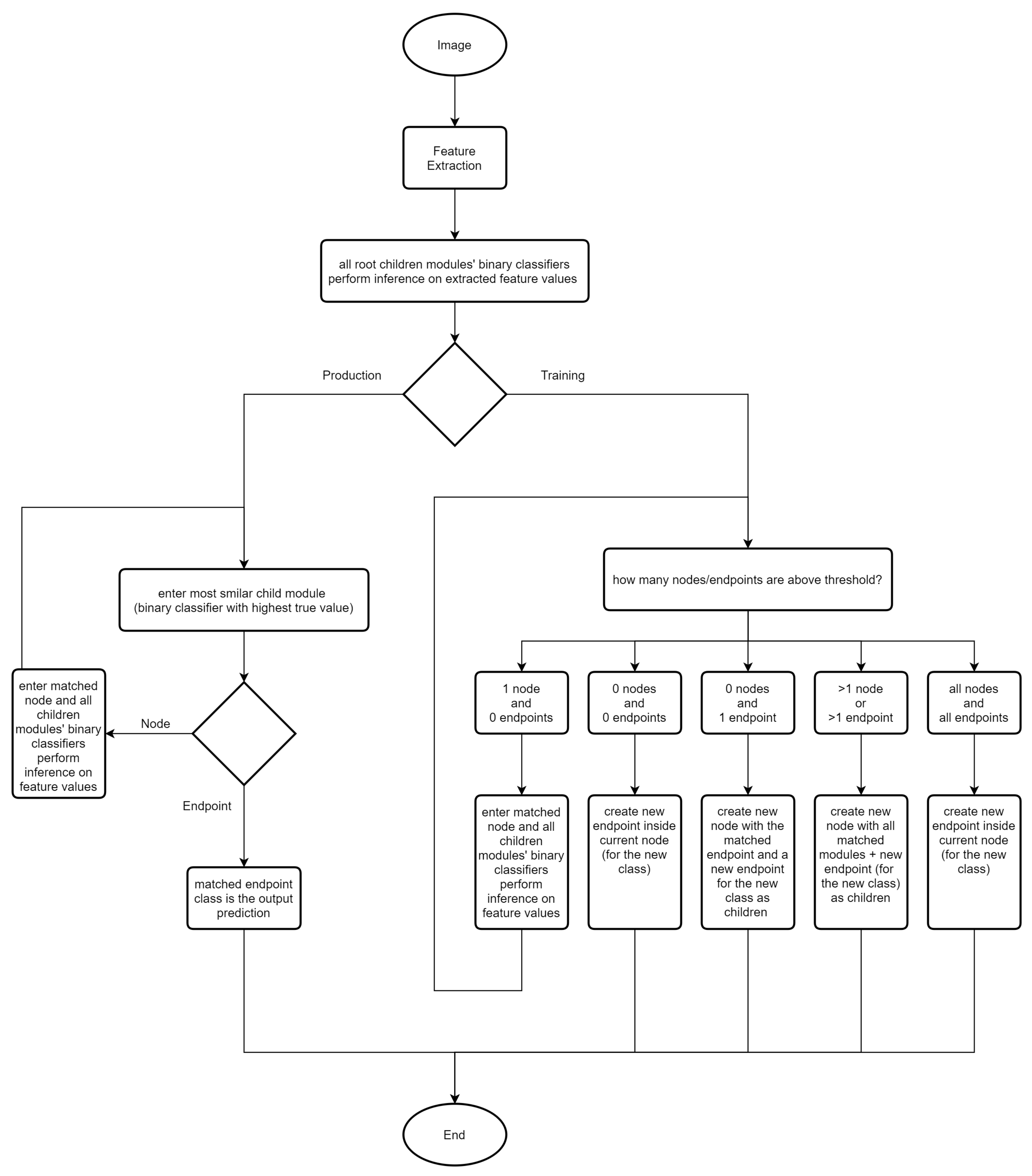
Figure 1 shows a global flowchart of the MDNN training and production processes, which are later explained in detail in the present section, where it can be seen that the feature extraction component is general to both training and “production” (inference) and how, based on decisions made by algorithms that are discussed in the paper, some recursive processes can occur.
For the first component of the network, (a) feature extraction, a pre-trained (ImageNet) ResNet50 [
1] was used as a backbone, which is known to provide excellent results for image classification; see [
24]. This component is only used for extracting generic “low-level” features, while smaller and more basic (modular) networks exist for extracting class-specific features in the dynamic classification component. The feature extraction part of the presented architecture is the only component that is never altered when new classes are being learnedbecause the modules in the next component rely on it to be consistent, so if the feature extraction part changed, they would be invalidated.
The second component of the network, the (b) modular dynamic classification component, is made up of numerous small modules. These modules serve the purpose of classifying specific classes or groups of classes that, as new ones are learned, are automatically split into groups of modules and sub-modules based on their class’s similarities. This grouping of classes can also be done manually if desired, but the standard operation of the network is to place them automatically based on the algorithms explained in
Section 3.2.
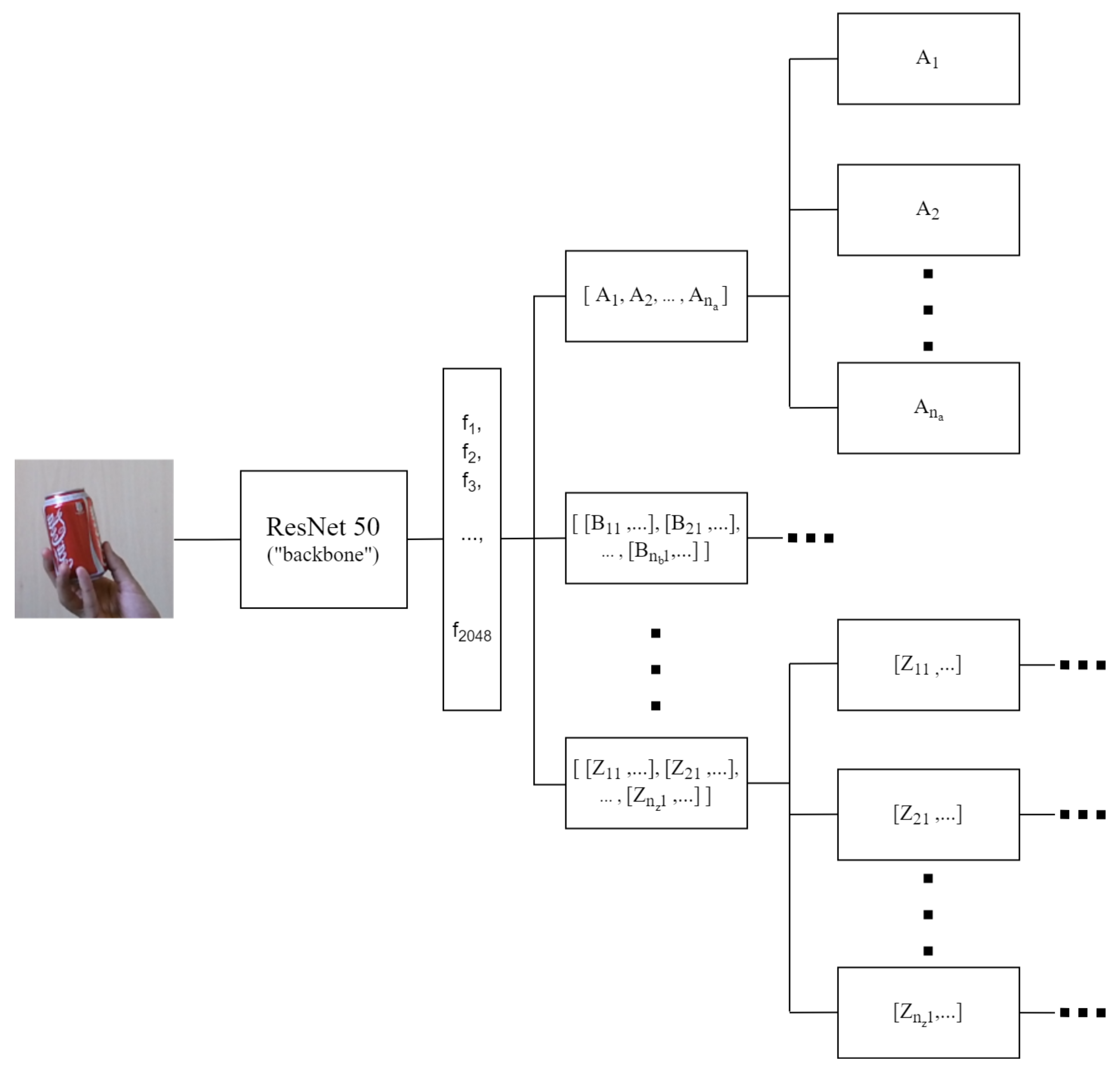
Figure 2 demonstrates how the modules fit into the proposed architecture: the modules with information inside brackets contain their own sub-modules (e.g.,
) or groups of sub-modules in the case of nested brackets (e.g.,
), where
to
are modules with no children and
represents the number of sub-modules belonging to their parent. The modules containing their own sub-modules are designated as
node modules and they have one binary classifier per direct child module. The modules with no children are named
endpoint modules and contain nothing but feature data obtained during the training process.
As the network learns new classes, the extracted feature values are stored within the
endpoint modules for future use, specifically for when some binary classifiers have to be retrained in order to avoid confusion with a new class. It is crucial to emphasize that the data preserved from each class are not the input data in their original format (“image”), but the resulting feature values obtained by the feature extraction component, which have smaller dimensions. In the case of the ResNet50, after being re-sized using nearest-neighbor interpolation, each sample image with a dimension of 224 × 224 pixels (px) and 3 color channels (224 × 224 × 3) is reduced to a 1 × 2048 vector (represented in
Figure 2 as
).
The module-based structure allows the network to grow dynamically while still being able to cope with the scalability-related issues that usually accompany dynamic approaches. This is possible because the modular structure makes it possible to make classifications without needing to use the entire network (see
Section 3.1). In addition, the fact that certain parts of the network are able to work independently from one another means that it is possible to add new modules or modify existing ones without affecting others. In short, the modularity of the networks’ sub-sections and each one being responsible for a given class or group of classes allow for parts of the networks’ knowledge base to be safely added, removed or altered without affecting the rest.
Finally, it is important to mention that other viable options could substitute the chosen feature extraction method (ResNet50), such as VGG16, Inception, or EfficientNet [
25,
26,
27]. In future work, tests will be done using feature extraction sections from different networks to compare them to each other. In the following sections, the modular dynamic classification component is presented in detail, as well as how the network is trained and how the stored data are used.
3.1. Modular Dynamic Classification
As mentioned, there are two different types of modules present in the presented arquitecture: (a)
endpoints, which are responsible for storing feature data extracted from a single class during training, and (b)
nodes, which contain references to two or more sub-modules along with a binary classifier (BC) for each one. Each sub-module can either be an
endpoint or a
node. The top part of
Figure 3 shows the difference between
nodes and
endpoints with a simple example of a potential network structure with three classes.
Each
node module has its own set of binary classifiers, which, in this case, are simple NN with two output values: a certainty value for “true” and a certainty value for “false” (both between 0 and 1), where the definition of what is true or false depends on the module in question and its location in the network. Each binary classifier represents one of a
nodes’ sub-modules. The binary classifiers that represent
endpoints define “true” as the only class they are responsible for, and “false” as the classes present in all the other modules and sub-modules in parallel with that
endpoint. The binary classifiers representing
nodes consider all of their sub-module classes as “true” and all the classes present in the other parallel modules and sub-modules as “false”. During the classification process, these binary classifiers are used to select which sub-module to continue with and end up defining a type of path that eventually leads to a final prediction. During the training process, they are used similarly to determine the best positions in which to “insert” new modules (see
Section 3.2).
Going back to
Figure 3, the bottom two rows show the same example as shown at the top but using a different representation, with the last one including an analogy with real-world objects. Classes B and C are joined as children of a
node (node [B, C]) and class A is on its own. This means that when this network was constructed, the algorithms in the training process calculated that classes B and C were similar to each other, grouped them together and trained new binary classifiers to distinguish between A and B ∪ C. Afterwards, a pair of sub-classifiers were trained to specialize in differentiating between classes B and C. To clarify, in this example, there are 4 binary classifiers present: A (against [B, C]), [B, C] (against A), B (against C), and C (against B).
Going into further detail, each binary classifier has the same structure, but naturally, different trained weights. In other words, the number of neurons per layer, the number of layers, the connections, the activation functions, etc., are all the same for every BC; the only difference between them is their trained weights. The main reason for this is to ensure consistency and provide all the BCs with an equal chance of success and avoid “favoritism”. This is important because both the classification and training processes have moments where comparisons are made between the predictions of the different classifiers.
The composition of the binary classifiers consists of six fully connected layers with the following numbers of neurons, 128, 64, 64, 32, 32 and 2, respectively, with rectified linear activation functions (ReLU), except for the last layer. The last layer’s activation function is a Sigmoid function. This is because the algorithms that use the output of these classifiers only make use of the true values, so there is no reason to let the false values interfere with the true values, which is what would happen in the case of an activation function, e.g., SoftMax. The architecture of the binary classifier, including the numbers of layers and neurons per layer, are determined empirically. In the future, this classifier will be the object of further studies in a way to improve the scalability of the network and save memory. It is important to justify at this point, the reason behind having a neuron representing the false value when it is not used. The reason is quite trivial: it is much more straightforward to implement and train a binary classifier this way, as this allows for the use of standard backpropagation for the true and false classes as if they were two normal classes. Nevertheless, in the future, the false values will be taken into account and also become part of the decision-making algorithms.
Figure 4 shows a more detailed view of the MDNN architecture (complementing
Figure 2): the left side shows the ResNet50 [
28] feature extraction, with the 2048 vector of extracted features, and the right side shows the network’s flexibility and how the number of sub-modules that a
node can have is not limited, including sub-modules of sub-modules. The figure also shows the use of the maximum value for deciding which sub-module should be used to continue the process. For the proposed network to meet its purpose of distinguishing between classes, the minimum number of classes for initialization is two. Therefore, the root module will always be a
node, as
endpoints only ever represent one class and
nodes are the only modules that can contain more modules.
It is worth remembering that whenever a binary classifier is called upon, no matter its position in the network, the input values will always be the same feature values (2048 length vector) which are extracted once from the data sample being classified. The positions of modules within other modules are symbolic and serve only to decide if and which other modules are to be used, but the extracted feature data are never altered. This is important to clarify because, when visualizing tree-like structures that are based on NN, one might easily mistake the presented architecture for a single network with a tree format, similar to what is shown in [
29], where everything is backwards dependent. Therefore, it must be emphasized that the “tree” serves only as a representation of the order in which things are done and which data are used by each binary classifier. The main takeaway from this is that the feature data are not altered intermediately, i.e., the input data for the last modules are the same as those for the first modules.
The nesting of modules within modules means that the classification process can be recursive. This is because, when applied to a node, the results dictate whether it should be re-applied to another sub-node, i.e., the classification process is (i) initially applied to the network’s root node and then, potentially, (ii) recursively applied to more nodes depending on the intermediate results.
So, to make a classification, the first step is for all the binary classifiers in the current
node to process the extracted features and then for all their outputs to be evaluated. Keeping in mind that these binary classifiers indicate the certainty that the input sample data belong to the module they represent, the application of the input sample’s extracted feature values to each of the binary classifiers (displayed in
Figure 4 as
, with
), results ina group of values between 0 and 1 (because of the final layer’s sigmoid activation function) that represent the likelihood of the input sample belonging to each of the modules in the
node being analyzed. Then, the highest value from these results is sought out, which indicates which module is the most likely to include the correct class. This selected module can then either be an
endpoint or a
node, where each one has a different next step. If the chosen module is of the
endpoint type, then the classification process ends here, and the output prediction is the class represented by that
endpoint. If, on the other hand, the chosen module is of the
node type, then it is necessary to enter that
node and keep repeating this process until eventually an
endpoint module is selected, resulting in a final classification.
This implementation plays a big role in one of the mentioned objectives, which is to avoid or at least attempt to minimize scalability issues. The main reason this implementation contributes toward this is because only the binary classifiers from the top-scoring sub-nodes are used, meaning that, for many cases, classifications are made using only a small percentage of the overall network. This means that, as the network grows, the classification speed is only slowed down for classes that get grouped with lots of other similar classes because they require a bit more time to be distinguished between them; for non-similar classes, only a very small fraction of time is required to make distinctions between them. In future work, the optimization of the classification process will be explored.
The next section is fundamental in understanding the architecture and explains how the network is trained (the second component; we stress that the first component, feature extraction, always remains unchanged—frozen), as it is not similar to the most “traditional” networks.
3.2. Modular Dynamic Training
The process for the addition of a new class starts (as usual) with the network being fed a set of data samples along with a label. With this, the network will (i) process the data samples, (ii) decide where best to place the new endpoint, (iii) make any necessary adjustments to the existing modules, and (iv) train the necessary classifiers so that when the network is presented with data from the same class, in the future, it can identify them.
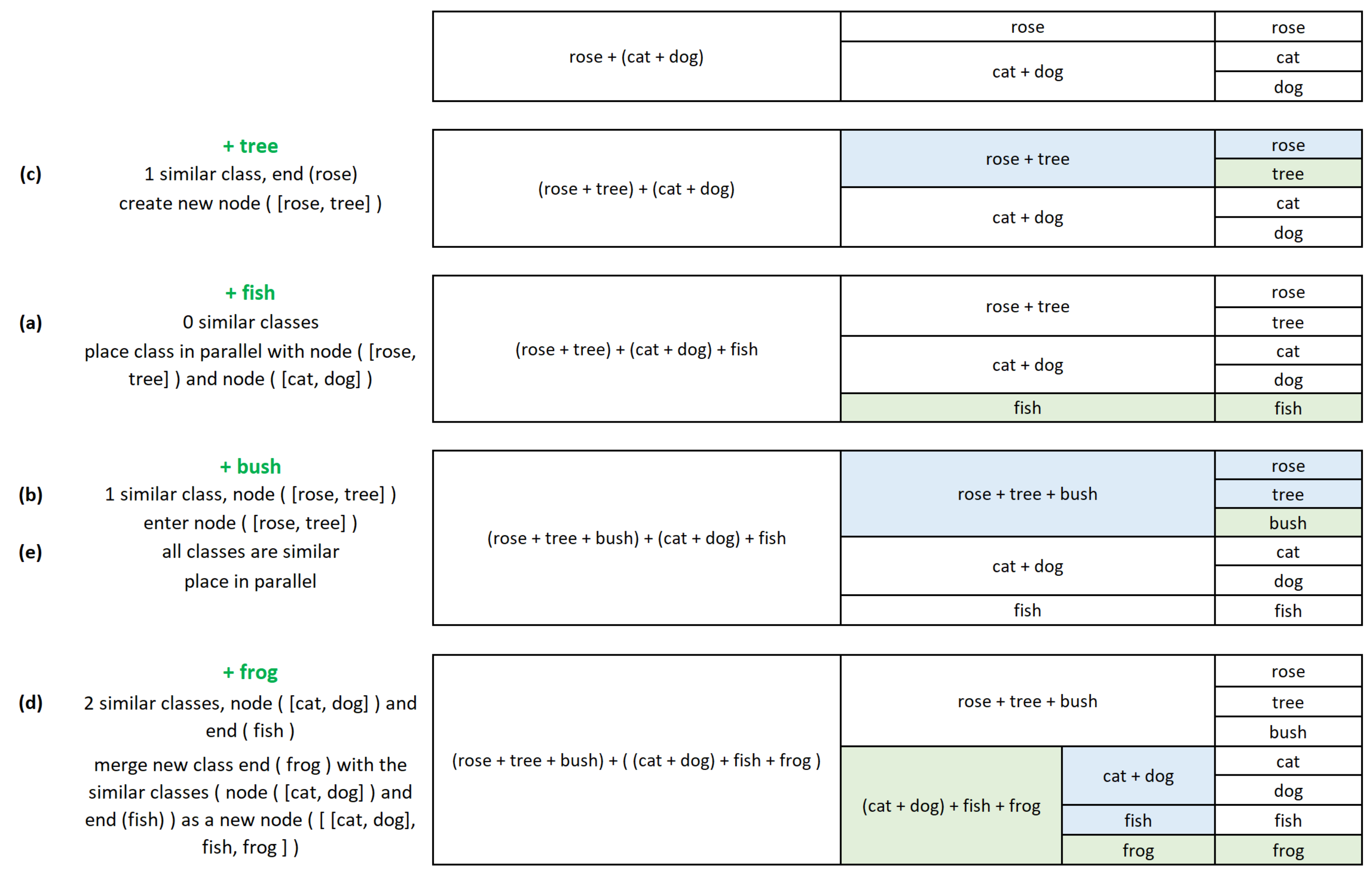
Following the scheme presented in
Figure 3, the right side of
Figure 5 shows an example of how the network changes as classes are added over time. Here, it is shown how it can classify three classes (shown in
Figure 3) (A—rose, B—cat, and C—dog), where B and C are grouped together, and then another four classes are added sequentially(D—tree, E—fish, F—bush, and G—frog), making the network capable of classifying a total, in this example, of seven classes.
The positions in which new modules are placed within the network are not random. There are several procedures behind the calculation of the optimal position for a new module (some of which can be recursive). Learning a new class essentially means that the network can distinguish the new class from the ones which were previously learned.
The most main goal of this class placement process is to avoid conflict or confusion between classes. In avoiding confusion between classes, the goal is to (i) group them by their similarities and then (ii) focus on their differences. This notion of grouping classes by similarities is referring to the parallel placement of modules within
nodes, as shown in
Figure 5, where, among other examples, in the network’s initial state, class B is grouped in a node with class C.
The binary classifiers are used to see if any existing classes share any resemblance with the class being added. The procedure for checking if classes are similar is relatively similar to the classification process, but instead of just searching for the most similar class, here, the goal is to search for any classes that could be partially similar, i.e., it looks for “somewhere” to place the new class.
Upon entering a node, there are n possible paths to follow, which can be a mix of endpoints and/or nodes. The idea here is that any node or endpoint binary classifiers that, without any alteration, might accidentally mistake the new class for their own should be grouped with that new class and retrained so that, in future, when presented with samples of the new class, they do not repeat the same mistake. To achieve this, it is necessary to first verify which nodes and or endpoints share any resemblance with the new class. Therefore, the first step here is to classify all the data samples (extracted feature values) of the new class with each of the binary classifiers in the current node and then use these results to decide how best to proceed.
After obtaining all the current node’s classifier results from all the new data samples, the next step is to calculate the average confidence per classifier, which returns a single value for each node/endpoint, representing the likelihood of mistaking the new class with the existing class (or classes if it represents a node). It should be noted that the use of the average for this task was a natural choice, but in the future, other solutions will be investigated in order to attempt to achieve even better discrimination between classes.
Next, the obtained average values are analyzed to see which classes are the most similar to the new one. Each value is compared with an established threshold value, , which makes it possible for a final decision to be made on whether a class should be considered similar, where this threshold value dictates the necessary confidence value for two classes to be considered similar.
To establish this threshold value (
), logic says it should not be too high because some similar classes could be missed, but should also not be too low so that only reasonably similar classes are considered. Different values between 0.1 and 0.5 were tested, and the best results were achieved with
= 0.3. These tests were done with three different datasets or subsets of those datasets, namely Core50 [
9], ImageNet [
12] and CIFAR-10 [
30]. The ideal value depends on how accurate the binary classifiers are and it essentially dictates how grouped or separated the final network is. Future work for this component includes the use of a dynamic threshold value that is re-calculated as the network expands.
After comparing the averages of the classifications of all the input samples with the threshold value
, it is known which, if any, modules are similar to the input class. This results in one of five possible outcomes in the function of how many similar
nodes and/or
endpoints are found (see also
Figure 5 left side): (a) 0 similar modules (0 similar
nodes and 0 similar
endpoints); (b) 1 similar
node and 0 similar
endpoints; (c) 0 similar
nodes and 1 similar
endpoint; (d) more than 1 similar
node and/or
endpoint but not all, and (e) all
nodes and
endpoints are similar. Each outcome is dealt with differently, as detailed next for each case:
- (a)
0 similar modules (0 similarnodesand 0 similarendpoints): Place a new
endpoint in the current
node for the new class. Train the classifier for the new
endpoint with true data as data from the new class and false data as a balanced distribution of data (see
Section 3.3 for the explanation) from the other
endpoints and
nodes present within in the current
node.
- (b)
1 similarnodeand 0 similarendpoints: Enter the similar node and repeat the positioning process on its children.
- (c)
0 similarnodesand 1 similarendpoint: Create a new
node and place a new
endpoint inside it for the new class as well as the
endpoint that was matched with the new class. Train the classifier for the new
endpoint with true data as data from the new class and false data as data from the class it was matched with (see
Section 3.3). Retrain the classifier for the pre-existing
endpoint that was moved into the new
node with true data as the data it has stored and false data as data from the new class.
- (d)
More than 1 similarnodeand/orendpoint: Create a new
node and place inside it a new
endpoint for the new class as well as all the
endpoints/nodes that were matched with the new class. Train the classifier for the new
endpoint with true data as data from the new class and false data as a balanced distribution of the data from all the other
nodes/endpoints it was matched with (see
Section 3.3). Retrain the classifiers for all the pre-existing
nodes and
endpoints which were moved into the new
node using balanced distributions of their own data as true data and balanced distributions of all their sibling’s data as false data. The child modules of the
nodes that were moved into the new
node do not need to be touched, as they are not dependent on their parents and only relate to each other.
- (e)
Allnodesandendpointsare similar: Place a new endpoint in the current node for the new class. Train the classifier for the new endpoint with true data as data from the new class and false data as a balanced distribution of data from the other endpoints and nodes present in the current node. Retrain the classifiers for all the pre-existing nodes and endpoints in the current node using balanced distributions of their data as true data and balanced distributions of all their sibling’s data as false data.
Out of these processes, case (b) is the only one that does not involve the placement of the new class or the training of any networks, but it repeats the entire process applied to a selected sub-node and, eventually, there is a point where there are no more sub-nodes and case (b) is no longer be a viable option; therefore, the new class is guaranteed to be placed somewhere in the network eventually.
After the new module is placed within the network, the parent node has to be re-trained so that it considers the new class as true, thereby increasing the chance of success for the classification process in production. This is because it increases the probability of future samples of the new class reaching the correct endpoint. The retraining of parent nodes must be recursive, i.e., the process must then also be applied to the parent of the parent until the root node of the network is reached. This process helps to ensure that the initial nodes are more likely to send samples of the new class down the correct path during production.
It is important to stress that the use of the same classifiers during the training process as those used during the classification of new data immediately makes huge improvements to the overall classification process. This is because with this strategy, it is possible to predict and correct the modules most likely to cause errors related to the addition of the new class before they are even a problem. The next section is dedicated to explaining how the data are balanced when train or re-training the binary classifiers.
3.3. Balanced Training Data
Research shows that neural networks have higher success rates when trained with balanced data [
31], meaning that they should be trained with a similar number of samples per class. As this architecture deals with binary classifiers (true or false), it should aim to use an equal number of true and false samples, leaving us with the problem of deciding what to do when there is a different number of each.
The algorithm implemented for the selection of training samples starts by calculating the maximum number of samples per class that can maintain an ideal distribution based on where they are positioned in the network. In this situation, where various groups of classes have their own sub-groups, an ideal distribution does not mean using an equal number of samples per class. It means the same number of samples should be used from each of a nodes’ children, i.e., if one of these children is an endpoint and one is a node, then the same number of samples should be used from each, where the nodes’ samples are a mix of their children’s samples and so on.
For example, recalling
Figure 3, if a classifier were trained to recognize an
endpoint A as true and a
node [B, C] as false, and A, B and C all had
m samples each, the balanced distribution of samples for this classifier would be
m samples of A and
m samples of [B, C]. Then, to continue aiming for an equal distribution, the
m samples of [B, C] would consist of
m/2 samples of B and
m/2 samples of C.
This example makes the problem appear straightforward, but with different numbers of samples per class and a more complex network structure (more known classes and more nested nodes on the true and false sides), an algorithm is needed for calculating the ideal distribution in any situation and making use of as many samples as possible. Using this equal distribution means classes with fewer samples will reduce the number of samples that can be used from other classes with more samples. So, to minimize this effect, it is recommended to establish a minimum number of samples (MNS) for when classes are added to the network. The currently applied MNS value was determined empirically and was set to 175; nevertheless, when using the MDNN architecture in a real-world situation, there is no knowledge of how many samples will be available per new class, and so a minimum value must be defined. Using MNS = 175 presented good results over the various tests performedand, during intermediate tests with the three datasets mentioned before, increased MNS values provided better results. Data augmentation would normally be a solution for increasing the amount of data available for the classes with fewer samples, but as the stored data consist of feature vectors and not raw images (as mentioned), the produced samples would not be reliable.
There are two main steps involved in computing the maximum number of samples to obtain a balanced training set: (i) calculate the largest number of samples that allows for the use of the distribution explained above and (ii) recursively divide this number by the number of children in a node until all endpoints are reached.
For the first step, (i), the number of sub-modules in the node is multiplied by the number of samples of the sub-module with the largest number of samples. The numbers to be calculated for the sub-modules which are also nodes are calculated in the same way. This means that the algorithm is applied recursively until all the sub-modules belonging to the node in question have been calculated and the node in question itself has also been calculated. When this process is complete, it results in the maximum number of samples that allows for an even distribution of samples for the node in question.
So, with
representing the maximum possible number of samples that can allow for an equal distribution for the
node being calculated,
represents the maximum number of samples that can be used by one of the
node’s sub-modules, with
p representing the path created by the indexations that lead to the location of the
node in question and
i being the index of a sub-module. For example, in the final state of the network shown in
Figure 5, the path required to reach the
node “[cat, dog]” would be the second sub-module of the root
node and then the first sub-module of that
node. Meaning that for the
node “[cat, dog]”, the indexations represented by
p would be “2,1”, and the number of samples present in the endpoint “dog” would be “
”. The value of
represents the number of sub-modules present in the
node being calculated, and
the number of samples which is computed (sometimes recursively) as follows:
The second step (ii) is to keep dividing equally between the children in nodes until all the endpoints are reached, resulting in the numbers of samples to use per class. For that, the value obtained from the first step is used, (the maximum possible number of samples that allows for an even distribution), and is progressively divided throughout the network. The node being calculated distributes its number evenly between its children. The children that are also nodes then do the same thing with their values to their children, resulting in sub-divided values. This is repeated until all the sub-modules of the initial node are reached and eventually results in a final number of samples to be used for each class . So, with the value of calculated in part one, it is possible to compute , which is essentially the value of evenly distributed between each of the node’s sub-modules.
While in step (i) the parent’s values depended on the the children’s values, in step (ii) the children’s values depend on the parent’s values. To initialize this process, the value for the node being calculated is set with and then its sub-modules values are calculated as . Afterwards, each sub-modules’ values are calculated the same way until all the endpoints that are descendants of the node being calculated are reached, which eventually results in a series of final numbers of samples to be used from each endpoint.
4. Tests and Results
One of the most common image classification datasets is ImageNet [
12]. In the literature, numerous benchmarks use this dataset, and others like it, where the networks/methods are trained to learn all the classes at once. Although their leaderboards show outstanding accuracy in their results, these are not the datasets and benchmarks used to validate CL methods. As mentioned, to validate continual learning architectures, we need to feed images (data/classes) to the network incrementally. To properly test a networks’ capacity for learning continually, a dataset and benchmark with pre-established CL-related rules and guidelines is needed; one of the most used datasets of this type is CORe50 [
9].
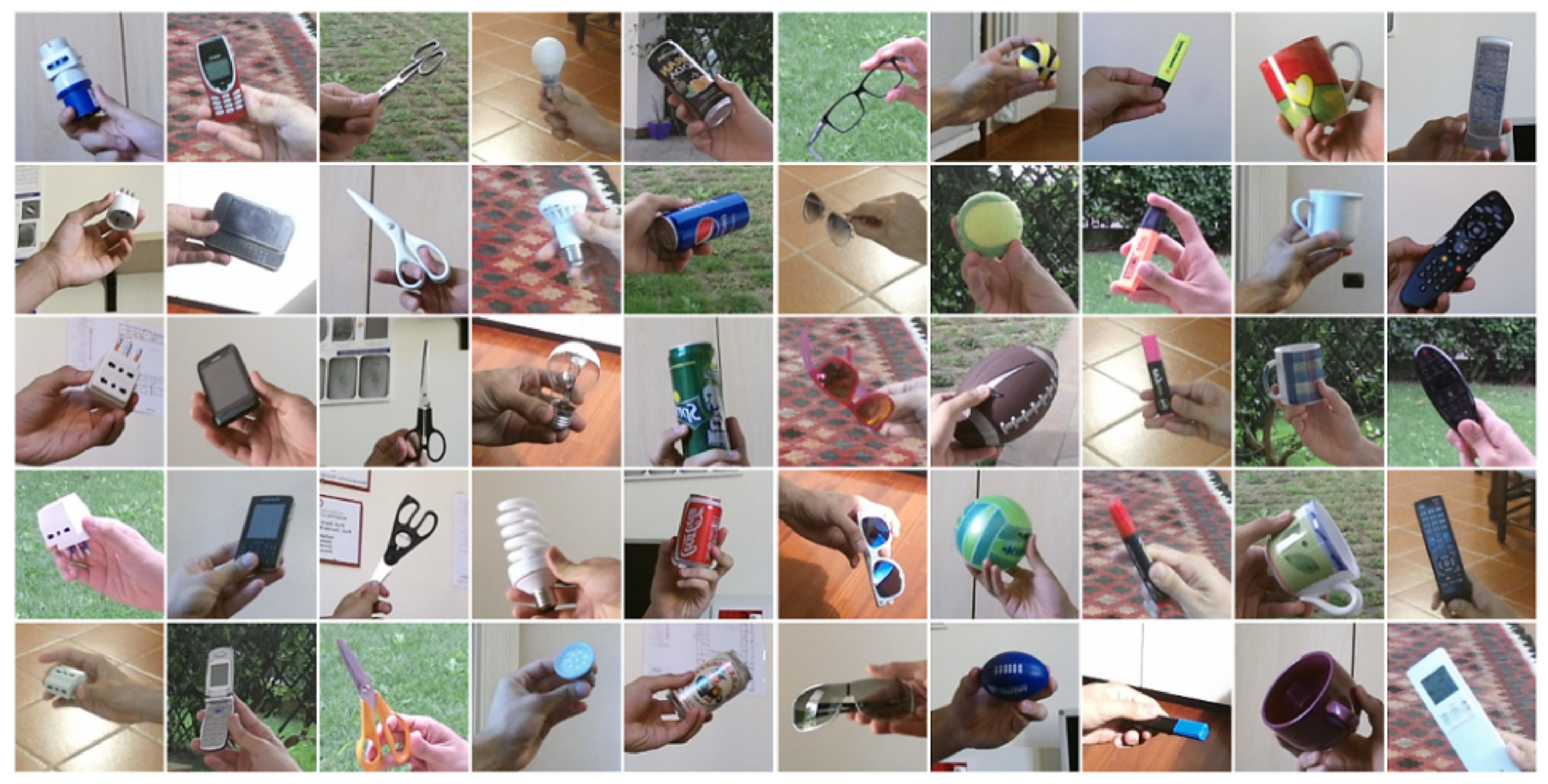
The CORe50 dataset consists of 50 classes (10 categories with 5 classes each). The 10 categories are as follows: plug adapters, mobile phones, scissors, light bulbs, cans, glasses, balls, markers, cups and remote controls.
Figure 6 shows an example of each class and how they are divided into the mentioned categories. The data were collected over 11 distinct sessions (8 indoor and 3 outdoor) characterized by different backgrounds and lighting. For each session and each object, a 15-s video (at 20 fps) was recorded using a Kinect 2.0 sensor producing 300 RGB-D frames. The objects were handheld by the operator, and the camera’s point-of-view is that of the operator’s eyes. The full dataset consists of 164,866 128 × 128 RGB-D images obtained from 11 sessions × 50 objects × (around 300) frames per session. More details can be seen in [
9].
In summary, each class has around 2398 training images and 900 test images which are split into various test/train batches (the number of batches and their contents depend on the CL scenario being considered). Here, batches represent sets of data (images) that are fed to the network in blocks [
9]. The dataset considers three continual learning scenarios: (a) new instances (NI), where all the classes are learned in the first batch and then new data for each class are added over the following batches; (b) new classes (NC), where the first batch includes 10 classes and then the following batches introduce 5 classes at a time until reaching the total 50; and (c) new instances and classes (NIC), where both new instances and classes are presented over time.
We opted to test our framework on the NC scenario, as its implementation is the one most comparable with the paper’s objectives. However, of course, we do plan in the future to implement the use of new instances to improve knowledge of already known classes, which will allow us to show results on NI and NIC.
As mentioned, the NC test begins with learning 10 classes and then continuing to learn more classes in groups of 5 until reaching a total of 50; this makes for 9 total steps. The first batch (the 10 initial classes) consists of one class from each of the 10 categories, and the rest of the batches consist of 5 random classes each (different for each run). We executed 30 runs of this test using the algorithms and parameter values described throughout this paper, where the feature extractor (ResNet50) maintained all its default parameters and pre-trained weights, the binary classifiers used the layer structure mentioned in
Section 3.1, and the minimum number of samples (MNS), which we typically set to 175, was not needed, as each class had a relatively large number of samples (approximately 2398 as mentioned above). The hyperparameters for the binary classifiers were as follows: RMSprop [
32] as the optimizer, the loss was set to sparse categorical cross-entropy, the metrics were set to only sparse categorical accuracy, 4 epochs, and validation split equal to 10%. The 30 runs were all that were executed, i.e., there was no preferential selection (cherry-picking). The tests were made on a 64-bit 3.20 GHz i5-3470 CPU accompanied by 8 GB RAM, and each run took between 12 h and 13 h (approximately 15 min per class). In the future, the whole process will be converted to be processed by GPUs, where it is expected that by using state-of-the-art GPUs, the framework will be able to learn new classes at a much faster rate, potentially approaching real time.
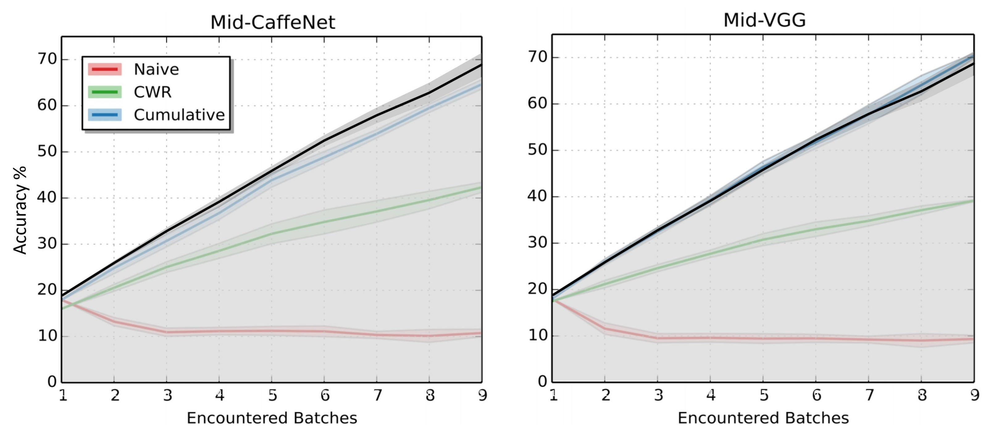
The graphs shown in
Figure 7, left and right, are adapted from [
9] and show the MDNN results obtained from the tests mentioned in the previous paragraph (black line) compared with three other methods. The copy weight with reinit (CWR) results (in green) are from the CL method presented in [
9]; naive (red line) simply continues training as batches become available; and cumulative (blue line) uses the current batch and all previous batches to demonstrate the potential accuracy of a network without CL restrictions and behaves as a kind of upper bound, but not quite, as Lomonaco and Maltoni [
9] state that “in principle a smart sequential training approach could outperform a baseline cumulative training”. Going back to the figure, the results we are comparing MDNN with on the left are based on a CaffeNet [
33] and the ones on the right are based on a VGG-CNN-M model [
34], but our results are the same on both graphs (the presented MDNN network was not based on a CaffeNet or a VGG, but simply structured as discussed in the paper).
When it comes to test data, Lomonaco and Maltoni [
9] considered what they refer to as a “full test set” where, at any moment during the continual learning process, the tests include all the classes from the dataset, so with that in mind, as the total dataset includes 50 classes and is initialized with 10 classes, the maximum possible accuracy is 20% and not 100%. So, where the x-axis in the graphs in
Figure 7 shows the 9 steps mentioned above and the y-axis represents the test accuracy at that point, after training on the first set of classes (step 1–10 classes) all the methods hover around 20%, which means that, based on the data available, they are all performing at close to 100% accuracy. The results shown in the last step (step 9–50 classes) are the accuracies achieved after adding 5 classes at a time and reaching 50 total classes. Here, when using the full test set (all 50 classes), as the networks were presented with all the training data, the accuracy values on this last step are a “normal” accuracy representation, where MDNN finished with 69.8% accuracy, and CWR ended just over 40% accuracy when based on a CaffeNet and just under 40% accuracy when based on a VGG. The cumulative results are similar to MDNN in both instances, showing that, in some cases, the presented network is capable of keeping up with (and outperforming) a method with no CL restrictions, i.e., demonstrating that based on the quote from before, “in principle a smart sequential training approach could outperform a baseline cumulative training”, and the presented approach can be considered “smart”.
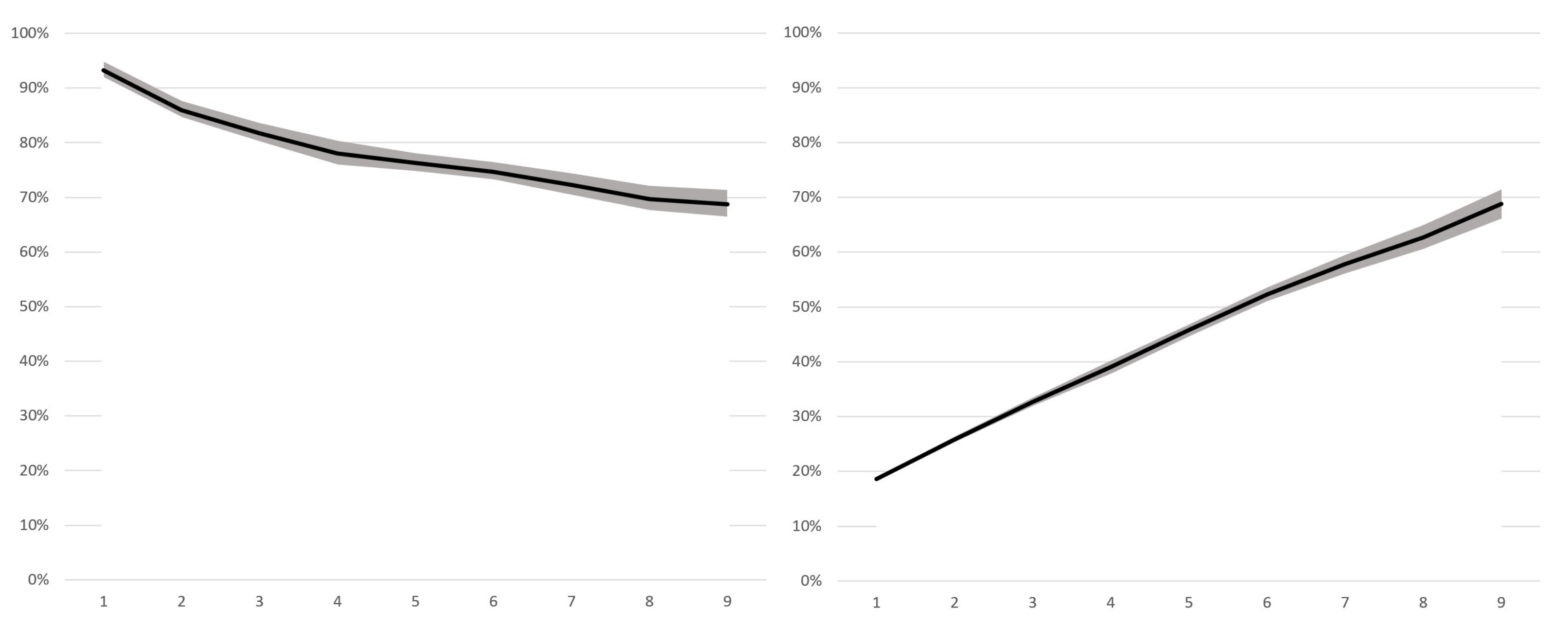
The left graph in
Figure 8 shows the average accuracy and standard deviation for each batch over time, where the tests at each batch are only of the classes supposedly learned, meaning that, in the first batch where 10 classes are learned, the network is only tested on its capacity to recognize those same 10 classes. In the same figure, the graph on the right shows the same results but considering the tests always being made with all classes (so when only 10 classes of the total 50 are known, the best possible achievable accuracy is 20%). The results are shown in both formats because the former (left) is how we think the results are the most understandable and gives a more clear idea of the networks’ overall performance over time, while the latter (right) is how the results were demonstrated in [
9], allowing us to make a more direct comparison.
The table on the left in
Table 1 gives a more detailed insight into the performance of the network by showing the individual results from each run and their accuracies over time after each set of 5 classes was added. The initial accuracy results from each run where 10 classes are learned sit between 84.4% and 96.5%, and the final accuracy results after all 50 classes are learned incrementally sit between 57.3% and 76.2%. It is also interesting to note that in some cases, the accuracy can actually be seen to increase when more classes are added (e.g., run 8 going from 35 to 40 known classes, there is a 7.4% increase in accuracy). Additionally, in
Table 1, the table on the right showcases all the increases and decreases in accuracy between each batch by using the same row/column representation but instead of showing the accuracy at each step, it shows the increase/decrease (delta) between the current accuracy and that obtained in the previous batch. Increases in accuracy are highlighted in green and decreases in accuracy are highlighted in red.
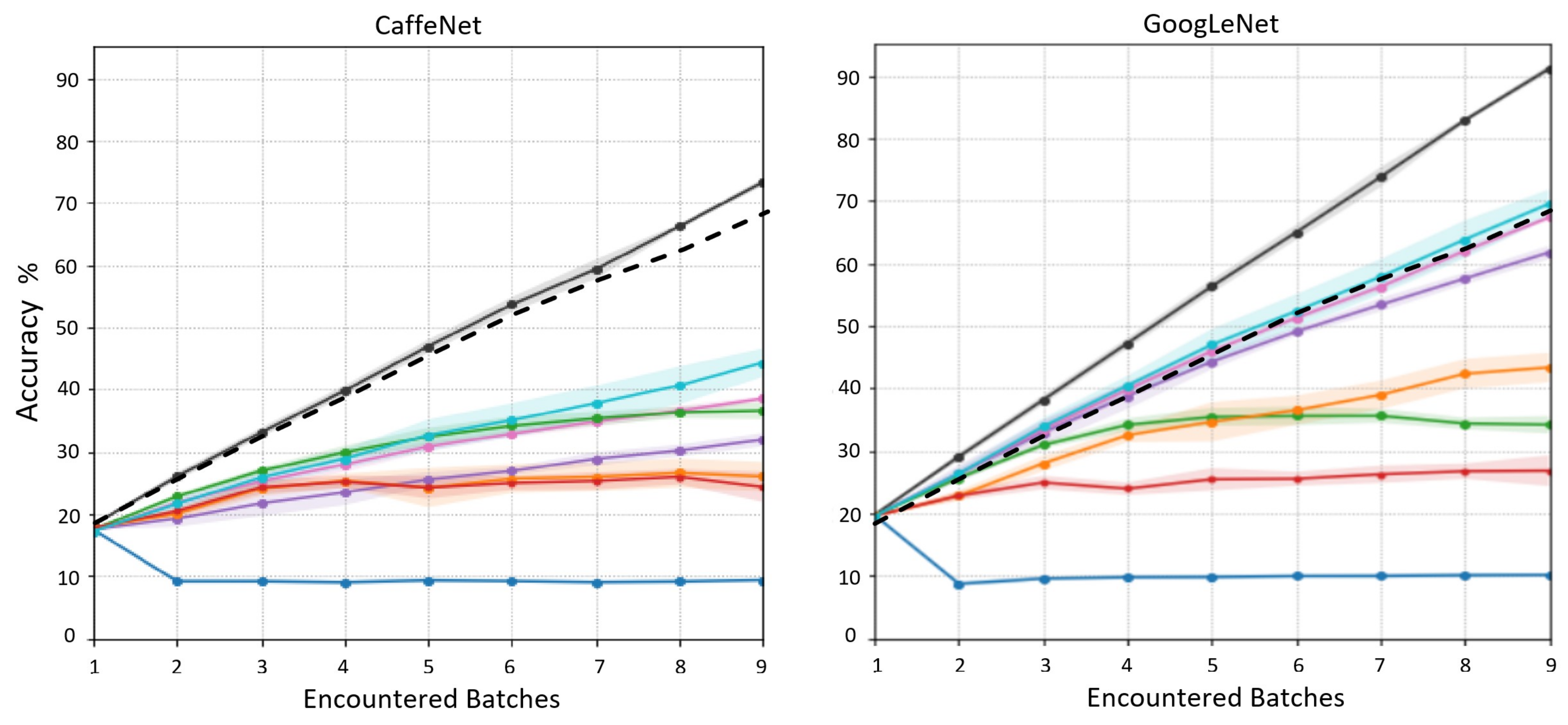
Figure 9 also shows the MDNN accuracy (dashed black line) on the CORe50 dataset, but this time compared with GoogLeNet [
35] using the following methods: cumulative (black line), naive (blue line), AR1 (turquoise line), CWR (purple line), CWR+ (pink line), LWF (green line), EWC (orange line), and SI (red line) (see [
14]). The dataset, context, and method of testing are all identical to those discussed in relation to
Figure 7. In the GoogLeNet comparison, our method no longer reaches as close to the cumulative result but is more in between AR1 and CWR+.
Before performing tests on CORe50, MDNN was also tested on ImageNet; although the dataset is not designed for testing CL methods, the test still provided some insights into the method’s performance. The test, shown in [
36], was made using 11 randomly selected classes. It consisted of the addition of one class at a time and evaluated the overall accuracy after the addition of each class. The test ended with 81% accuracy, where the average was brought down by two similar looking classes that generated confusion between each other (alyssum and astilbe). On top of that test, two additional classes (not from ImageNet) were added to the same network to measure the performance of the network when learning from multiple sources of data. The overall accuracy after the additional two classes were added was 82% and none of the pre-learned classes appeared to be negatively affected.
As the bottom line, a framework is presented that can learn new classes without the need to retrain its entire network of classifiers, with features that help it to cope with the scalability problems that generally come with expanding architectures. The test results on the CORe50 dataset [
9] show accuracy results just under 70% and in the case of comparisons against VGG and CaffeNet based models, MDNN was even able to practically match and even surpass results obtained on the same data without CL restrictions. The tests show that the framework has the ability to learn classes incrementally and to maintain its accuracy on old classes as new ones are added, making sure they are not forgotten.
5. Conclusions and Future Work
This paper presents a modular dynamic neural network framework: a continual learning solution that allows new classes to be learned incrementally, growing and structuring itself as it learns while re-training only specific sub-modules as needed. This way, parts of the network are not altered, allowing them to retain their knowledge.
The idea of constantly adding new smaller neural networks to a global main network creates initial concerns for scalability, but the network is structured in such a way that different parts are used for different tasks, which considerably reduces the severity of this problem. In addition to this, the architecture functions in a completely different way compared to other CL methods. The most similar one is LR [
22], where the main differences are that (i) their feature extraction component is not static (its alterations are sometimes slowed down during training), where for MDNN, that component is permanently fixed so that the MDNN binary classifiers maintain validity. (ii) When they train new classes, they re-use their stored samples from already known classes. This means that their high-level feature extraction is not affected too badly for old classes by the slow training of their low-level feature extraction. The presented architecture also re-uses samples of already known classes during training but only from particular classes in specific cases, where it depends on the location of the module in question. Finally, (iii) the classification part of their network is made up of one NN of fixed size, whereas the presented architecture is made up of multiple NNs with more being added progressively as needed.
In terms of future work, as mentioned, the framework is made up of many different components, which leaves us with several areas that can be improved in terms of performance and adaptability. The main six (future works) are presented in detail:
(a) Scalability and memory usage. With the elimination of catastrophic forgetting being the main focus (and the consideration of memory and network size constraints as secondary goals) priority is given to accuracy over scalability. While the presented approach does make efforts toward scalability and performance-related issues by using only the necessary sub-modules in both the training and classification processes, there is still more that can be done by attempting to reduce the dimension/quantity of the stored features and by attempting to reduce the algorithmic complexity of each module.
(b)
Feature extraction. The currently implemented feature extractor (ResNet50), while very performant, is not the only option for this task. As mentioned, there are other viable solutions that could substitute it, such as VGG16, Inception, or EfficientNet [
25,
26,
27]. The type of feature extractor also depends greatly on the data being used. One of the ideas behind the structural separation between the feature extractor and the modular dynamic component is that the feature extractor can be altered to whatever is best suited to the data being dealt with, so, for instance, to apply MDNN to problems other than image-related ones (such as audio, NLP, etc.), theoretically, one would only need to alter the feature extractor (and, of course, the binary classifiers would need to be structured to have the same input format as the feature extractor’s output). With this in mind, there is much work to be done to achieve and prove/validate this claim.
(c) Binary classifiers. The binary classifiers implemented here are relatively simple neural networks, and, like most other neural network applications, their structure and parameters could be subject to a lot of alterations and still perform equally, making it hard to know the “ideal” structure for any given situation. However, while an ideal structure for each application is not necessarily known, there is still room for work to be done and tests to be made concerning the binary classifiers seen here and to also look into alternative classification methods (instead of neural networks).
(d) New module placement. The placement of new modules considers the average accuracy value obtained by the binary classifiers using all the training data provided. This method has proven to be functional, but some factors could be taken into account to improve this algorithm. For instance, when the resulting similarity results from a set of training data show a large standard deviation, this could indicate that only a sub-sample of the class being learned is considered similar, and the current algorithm would not account for this fact.
(e) Usage of new data of known classes. Currently, the architecture is not prepared to make use of new data of an already known class. Once a class is learned from a certain set of training data, that is it. The implementation of this feature will consist of preparing the binary classifiers to resume training, the selection of which binary classifiers to continue training (and how much they should be trained) and also the calculation of when to re-arrange/re-structure the network in face of new data, e.g., upon continuing training parts of the network with new data, new intermediate test/validation results could show that some of the classes it considered to be similar are, in fact, not as similar as initially predicted and this situation could benefit from a re-structure. The implementation of this feature will also allow us to make comparisons with other methods’ results achieved on the NI and NIC benchmarks from the CORe50 dataset.
(f) More tests using different datasets. Finally, after doing the total or partial improvements mentioned in (a–e) we will also test the method using different CL datasets.
In a final summary, this paper presents an extension to an initial proof of concept for MDNN [
36] that showed test results from ImageNet, which revealed it to be a viable continual learning approach. Now, the present framework is detailed, improved, validated and tested on a CL-specific benchmark. It is possible to conclude that the framework presents similar or better results when compared with the state-of-the-art CL architectures. Nevertheless, the framework still has space for improvement and the potential to achieve even better performance results with real-time data, CL datasets and standard datasets.


