1. Introduction
1.1. Research Background and Necessity
Welding is an essential technology in industry and provides metals for applications in the building of ships, aircrafts, and automobiles. In the shipbuilding and offshore plant industry, welding is a major part of the production process, and it is important to inspect the condition of the welds because the weld zone affects the strength and durability of the structures. Non-destructive testing technologies are primarily used to determine the quality of the weld zone. Representative non-destructive testing technologies include radio-graph testing, ultrasonic testing, magnetic particles testing, liquid penetrant testing, eddy current testing, leak testing, and visual testing [
1]. Radiographic testing and ultrasonic testing are especially used in the shipbuilding field [
2]. Radiographic testing is the most preferred method by ship owners as the resulting images can be stored permanently, and the interior of the weld zone can be examined visually.
Currently, to collect information on welding in several shipyards, people are directly checking welding inspection information on shipbuilding and offshore plant structures of as many as 500 blocks or more. To inspect and determine the quality of the weld zone, experts as well as considerable time, expenditure, and manpower are required to manually examine the weld images. Additionally, the checking of the weld zone and information, is subjective and made through experience, resulting in inconsistent and irrational results. If deep learning could be used to automate the extraction of the weld bead shape, it would save considerable time and money, and efficient quality inspections could be conducted. As a result, objectivity can be secured in the quality inspection and determination of the weld zone in the shipbuilding and offshore plant industry. Depending on the bead and base metal generated in the welded area during a welding operation, areas with the same shape may be classified as different types of defects. Therefore, when determining the weld quality, it is necessary to efficiently perform inspections and determine whether the weld zone has defects or inadequate quality by extracting only the bead from the weld image and identifying the bead’s generation pattern.
Algorithms that extract only weld beads from the radiographic testing image have been used to perform weld detection via image preprocessing; however, they have been inefficient owing to noise outside beads that occurs via thresholding, which requires the algorithms to perform the additional task of removing the noise [
3,
4]. Additionally, image preprocessing methods including noise reduction, contrast enhancement, thresholding, and labeling, were performed to segment only bead from the radiographic testing image [
5]. In the image where thresholding was performed, the boundary of the bead area was defined and the edge was extracted to segment only the bead area [
6,
7]. Attempts to extract only beads from the radiographic testing image are continuously being made in various ways. However, since several tasks are performed manually, efficient tasks are not performed. It is difficult to say that the weld bead was extracted automatically. Therefore, it takes a lot of time and money to extract the weld bead and detect weld defects. This study aims to automatically segment the shape and location of the weld bead from the radiographic testing image through deep learning and the extracting of only the weld bead. To accurately detect weld defects, the weld bead must be extracted from the radiographic testing image, and this task can be performed efficiently if the weld bead extraction is automated.
1.2. Research Methods
This study used the deep learning-based U-Net [
8] algorithm to automatically examine weld bead shapes in radiographic testing images and determine the shapes and locations of the beads for detailed defect classification. For increased accuracy of the bead detection, image preprocessing was performed via histogram equalization [
9] to improve the contrast of the images before the model training. Furthermore, to diversify the data and improve the deep learning performance, data augmentation was performed to artificially expand the image data [
10]. It was checked whether the performance of deep learning was improved through training results before and after image preprocessing and data augmentation were applied. The weld images were captured using radiographic testing, and the radiographic images were marked with information to classify and distinguish them. For training, mask images were created by performing a labeling process that removed areas other than the bead area from the weld images. The weld images and the data with labeled bead areas were combined to create the training dataset to train the bead areas, such that the bead shape extraction could be automated. The images that constituted the dataset were divided into training and testing images to determine the training accuracy. The images had a variety of pixel sizes of approximately 1030 × 300 or greater. It was found that high-quality images reduced the learning speed. To efficiently train the images, the image pixel sizes were reduced to 256 × 256, then training was performed [
11]. After completing the training, the shapes and locations of the predicted weld beads were compared to those of the actual beads. Image post-processing was performed from the predicted bead shape and location image to extract only the weld bead.
2. Methods
Given the properties of radiographic testing images, the current conditions during the process of converting analog images to digital images via scanning may result in varying image quality. Additionally, it is necessary to have a method that can extract various weld bead shapes from limited data as it is difficult to collect a large amount of data owing to security concerns. To resolve these two complications, this study utilized a preprocessing method that changed various types of images into standardized images, and a data augmentation method that artificially expanded the data to avoid the problem of overfitting that can occur while using a small dataset during deep learning.
2.1. Contrast Limited Adaptive Histogram Equalization
In weld images that have been captured by radiographic testing, there are cases where the weld zone cannot be seen clearly as the image is too dark, and it is difficult to extract the weld bead shape. Therefore, this study used a histogram equalization (HE) method as a preprocessing technique to improve the contrast of the image by changing the image’s pixel distribution. HE adjusts the image’s histogram so that the pixel intensities that are concentrated within a certain range are distributed evenly. However, because HE redistributes the pixels of the image using a single histogram, it can only be performed if the pixel distribution is the same throughout the entire image. Furthermore, because various bright and dark areas exist in the image, the image may become overly bright or distorted when HE is performed. To compensate for this, the contrast-limited adaptive histogram equalization (CLAHE) [
12] was developed. CLAHE is a method that divides the image into several blocks of a fixed size and performs HE on each block to compensate for the challenges of the normal HE. As shown in
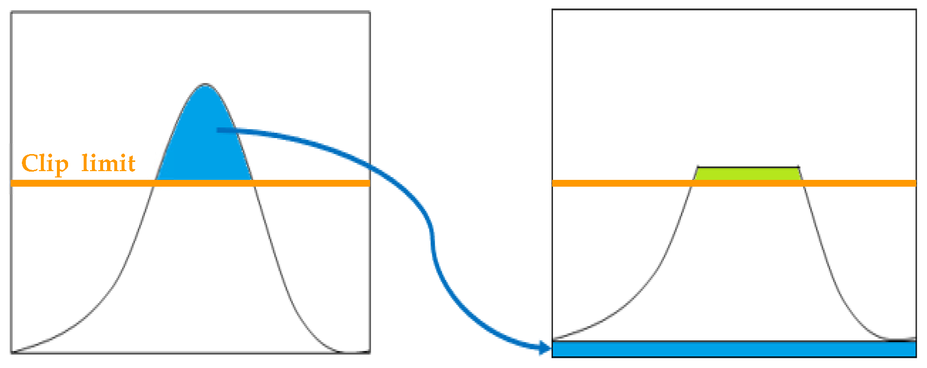
Figure 1, it undergoes a process of redistributing the pixel intensities that are above a certain height in the histogram. A value that limits a certain height in the histogram is called clip limit. Clip limit depends on the normalization of the histogram and thereby on the size of the neighborhood region, and is usually set between 3 and 4.
2.2. Data Augmentation
Data augmentation is a technique used during deep learning that artificially expands the dataset when there is a small amount of data available for training. Using an insufficient amount of data for deep learning can cause overfitting, which may reduce the deep learning performance. Moreover, for a deep learning model to generalize the test data efficiently, more data must be used for training. Therefore, it is necessary to expand and diversify the data based on the dataset that has already been procured to improve the learning performance of deep learning. Standard data augmentation methods include various techniques such as rotating, cropping, flipping, and adding noise to images. The data conversion efficiency of these methods has already been verified in several studies [
13].
2.3. U-Net
In recent years, several studies have been conducted on image segmentation techniques owing to the increasing interest in self-driving vehicles and object recognition [
14]. Deep learning models are often used for video and image segmentation. U-Net is an end-to-end fully convolutional network-based model [
15] designed for image segmentation, and has been used for image segmentation in applications such as X-ray and magnetic resonance imaging (MRI) [
16].
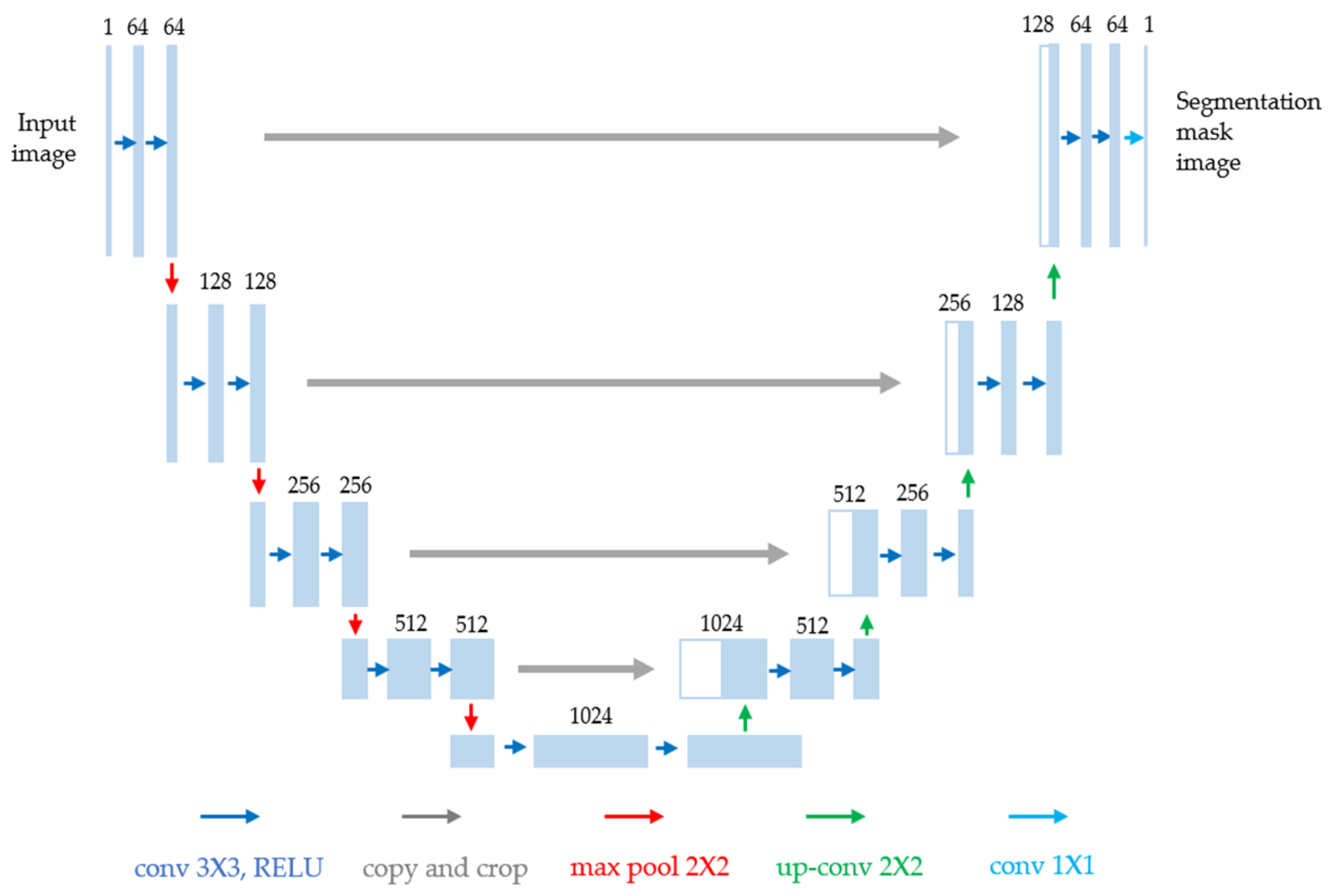
U-net has a U-shaped network configuration, as shown in
Figure 2. As it uses a convolutional neural network (CNN) [
17] structure, it contains several layers and extracts features from images. After extracting the features, transpose convolution is used to begin the image segmentation based on these features. The U-shaped structure can be broadly divided into three parts. The first is the contracting path, which examines a broad range of image pixels and extracts context information. The second is the expanding path, which combines context information with pixel location information (localization) to distinguish the object to which each pixel belongs. The third is the bottleneck, which converts the contracting path to the expanding path.
In the contracting path, a downsampling process is repeated to generate a feature map. The bottleneck is the segment that converts the contracting path to an expanding path. In the expanding path, the feature map is upsampled. Additionally, the expanding path performs the role of combining the contextual information that was generated in the contracting path with the location information using skip connections. If the size of an image is reduced and increased again, detailed pixel information is lost, which is a major challenge in segmentation requiring dense pixel-by-pixel predictions. Clearer image results are obtained from the decoder part through the skip connections, which directly pass important information from the encoder (contracting path) to the decoder (expanding path), allowing for more accurate predictions.
3. Data and Training
3.1. Data Configuration
In this study, 500 weld images were obtained for use in the experiments, and the CLAHE image preprocessing technique was used to improve the contrast of the weld images. The 500 weld images were from three in three different shipyards and each shipyard had own radiographic testing environment such as X-ray energy.
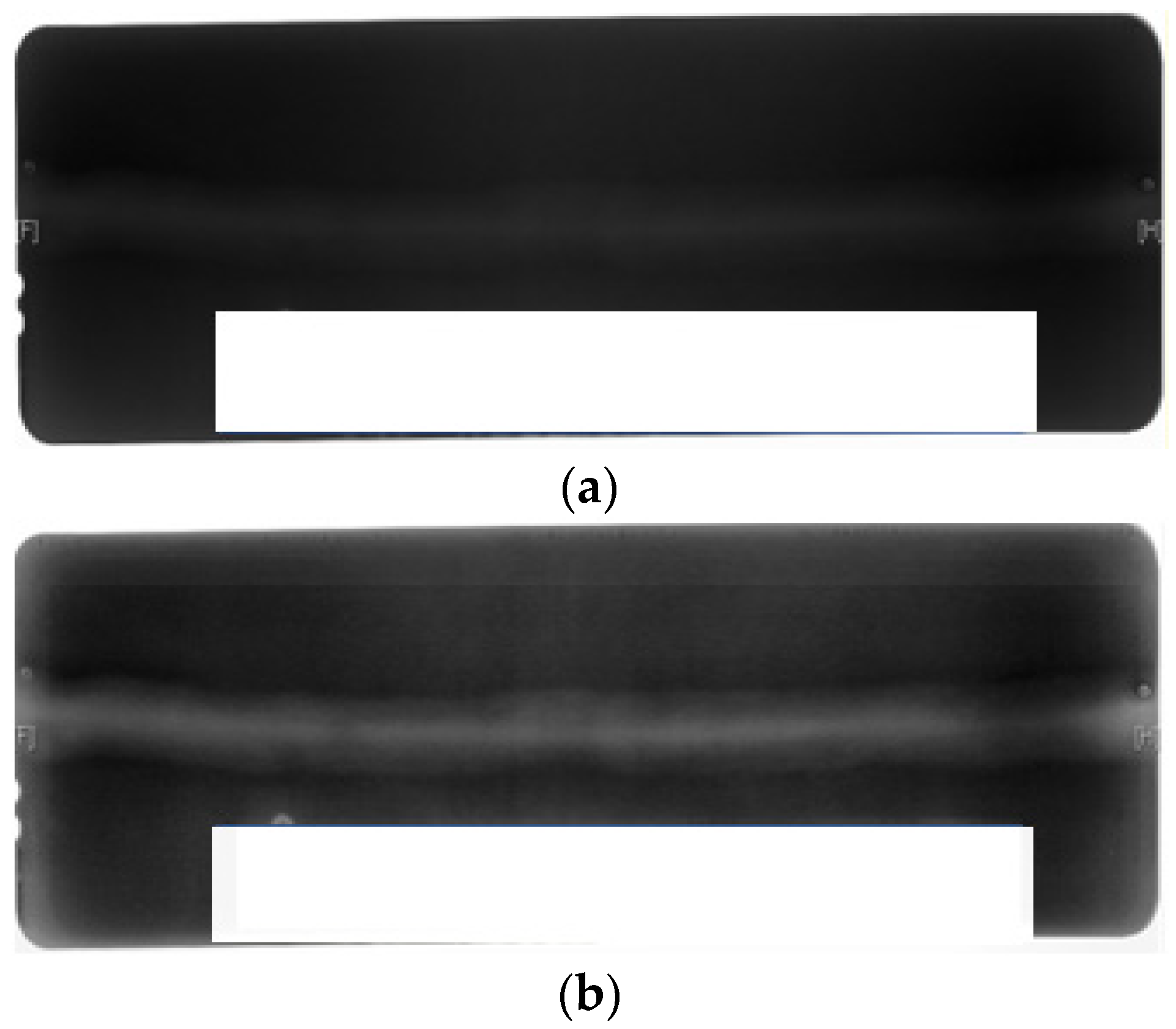
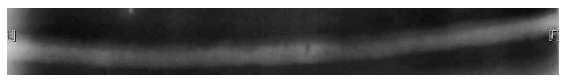
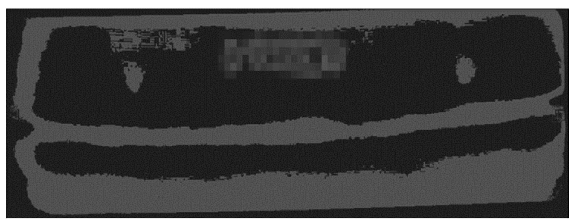
Figure 3a,b show the original image and the image after CLAHE was performed, respectively. In the images presented in this paper, there is a white rectangular box, which covers the information about the radiographic image for security.
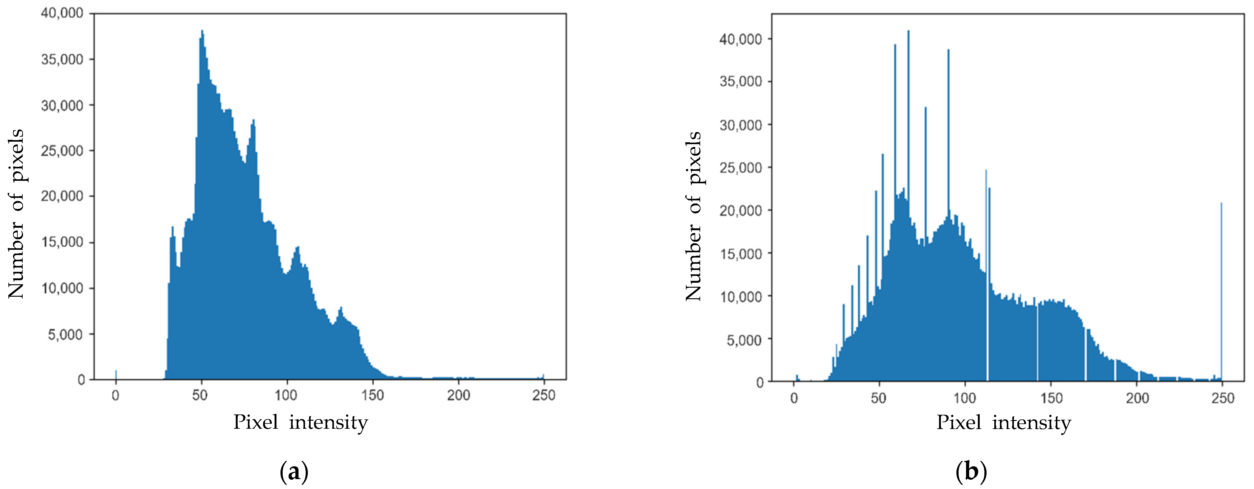
Figure 4a,b show the histograms of the original image and the image after CLAHE was performed, respectively. Furthermore, among data augmentation techniques, rotating, cropping, flipping, and brightness adjustment were used to expand the weld images to a total of 2500 images.
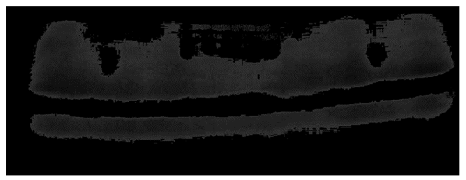
This study also used mask images as training data for the U-Net model. Mask images are created by performing a labeling process. These mask images only contained pixel intensities of 0 or 1, where 0 indicates the area outside bead and 1 indicates the bead area.
Figure 5 shows a binary mask image in which labeling is performed on the image presented in
Figure 3b.
When image data are read, the images are saved in PNG and JPEG formats, and the label information is saved separately. Additionally, when images are read in the PNG or JPEG format and encoded and decoded several times, significant performance reductions occur in the training stage, which become an inefficient part of the process.
To perform the training efficiently and improve the speed, the weld images were combined with the mask images that had gone through the labeling process and contained only the 0 and 1 values, and the Tfrecord files were created. A Tfrecord file is a binary data format for storing TensorFlow training data. Tfrecord files allow the management of the training data and the label information in one file. Tasks such as encoding and decoding can be batch processed in a single file, eliminating the need for additional work and increasing the training efficiency and speed [
18]. The weld images and mask images are encoded into a Tfrecord file, and the width and height of the image are additionally saved. Additionally, the encoding format is set to bytes.
The most common method for evaluating deep learning models is to divide and use the collected data [
19]. The 500 raw images and 2500 images after data augmentation was performed were divided and specified as the training and test dataset: 350 and 1750 images were used for training, and the remaining 150 and 750 images were used for testing. Of the collected data, the training data were used in the model training process. The test data were used to deduce the model’s performance; that is, how well the model learned using the training data.
3.2. Deep Learning Model Training
U-Net was used to extract the features from the weld images and predict the shape and location of the weld beads. For training, U-Net received weld images and mask images that would become the training target images. The original weld images and mask images that would become the training target images were combined into the Tfrecord files, and these were used as the training dataset. High-quality images reduce the training speed, making it difficult to achieve good performance as there are many parameters that must be learned. Therefore, to perform training efficiently, the image pixel sizes were reduced to 256 × 256 before training was performed. Additionally, the input images were normalized to (0,1), and the activation function of each layer was set up so that ReLU [
20] was used to apply the normalized values. The training was performed with a batch size of 1 and a learning rate of 0.00001; 18,000 iterations were performed. Binary cross entropy [
21] was used as the loss function, and Adam [
22] was used as the optimization function. Algorithm 1 shows a detailed algorithm.
Table 1 presents hardware and software for the experimental environment. Depending on the hyperparameters and the experimental environment, the time required for the experiment varies. The model was trained using only the training dataset, and the trained model was tested using the test dataset.
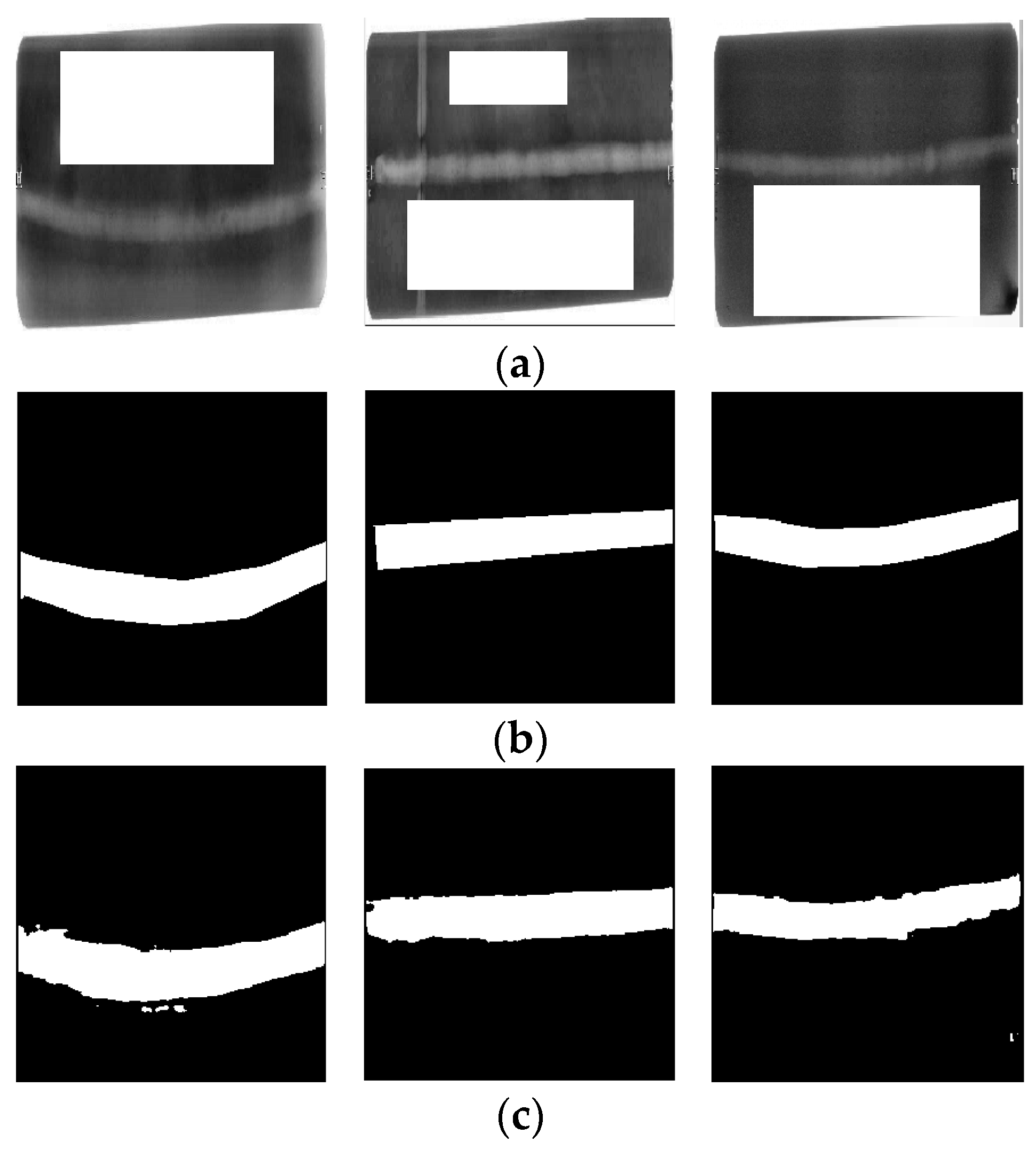
Figure 6 shows the results of testing the model that trained 2500 images in which CLAHE and data augmentation are performed: (a) is the actual weld image used as the input, (b) is the actual mask image, and (c) is the mask image that was predicted via the training process.
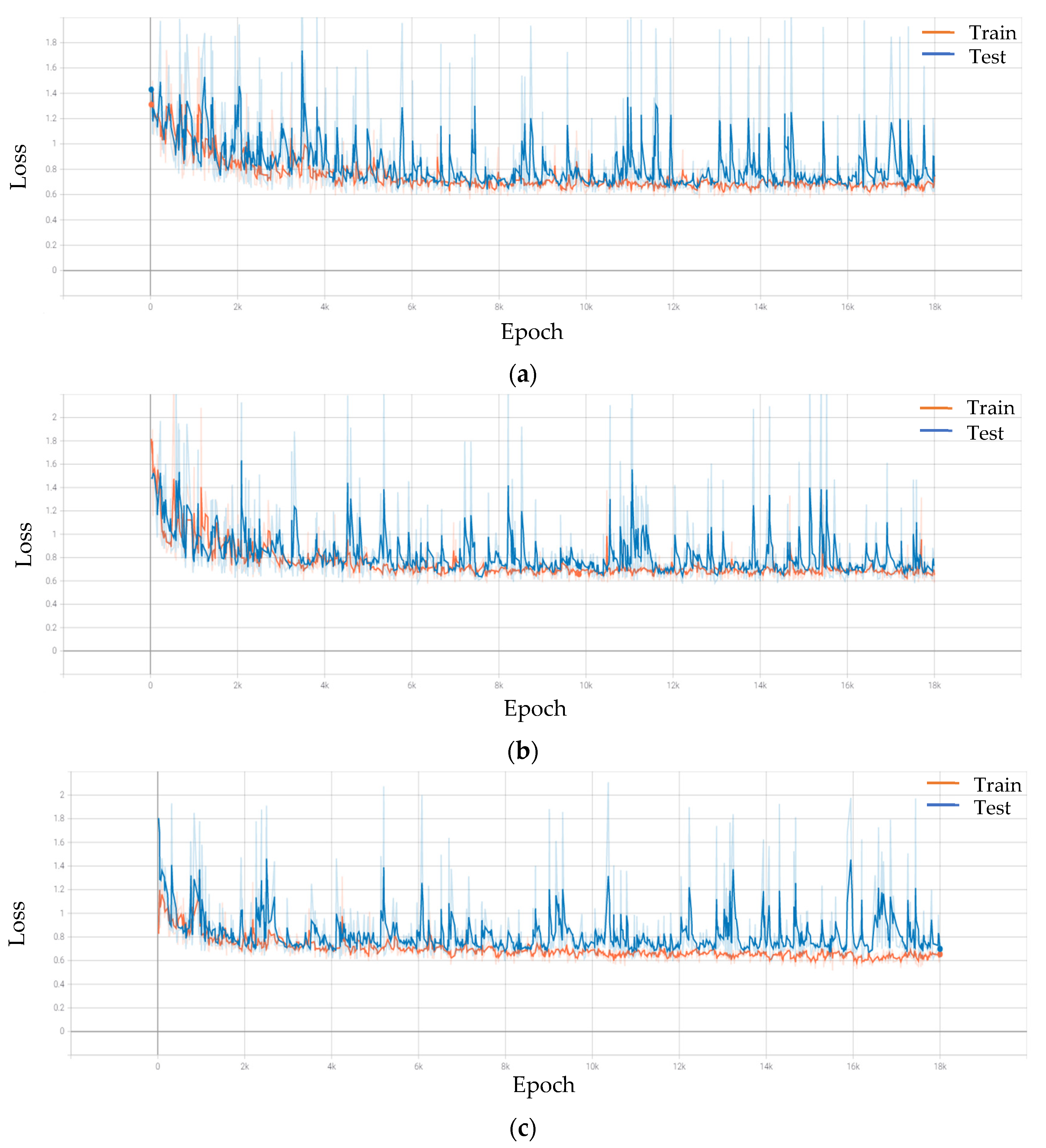
Figure 7 shows the loss functions of the training and test data.
Figure 7a shows the loss function when training 500 raw images,
Figure 7b shows the loss function when training 500 images in which CLAHE is performed,
Figure 7c shows the loss function training 2500 images in which CLAHE and data augmentation are performed. From the loss function, it can be determined that overfitting did not occur in the model.
| Algorithm 1. Learning for image segmentation. |
| Input: Image pixel feature , , and training step .
|
| |
| Output: U-net model parameters , Predicted values .
|
| |
| Loss function: |
|
|
| |
| Optimization: Adam |
| Require: : Step size
|
| Require: |
| Require: Model parameters |
| (Initializer initial moment vector)
|
| (Initializer initial moment vector)
|
| (Initializer timestep)
|
| While not converged do |
| |
| |
| |
| |
| |
| |
| End While |
| Return (Resulting parameters) |
4. Results
4.1. Experimental Results
To evaluate the performance of the image segmentation model, this study used the intersection over union (IoU), mean intersection over union (mIoU), and pixel accuracy [
23], which are evaluation methods from the PASCAL visual object classes (PASCAL VOC) [
24]. The values of each of these parameters were obtained for each pixel.
Table 2 depicts a comparison of the actual and predicted values to measure the performance of the trained model. The IoU is an evaluation index that measures how well the predicted bead shape and location in the weld image match the actual bead shape and location. Specifically, the IoU measures how well the areas with a pixel intensity of 1 match when comparing the mask image and the predicted image, as shown in Equation (1). The mIoU is the average of how well each of the bead areas and base metal areas match, as shown in Equation (2). The pixel accuracy is a number that expresses the accuracy of the prediction with respect to the entire base metal in the weld image, as shown in Equation (3).
Table 3 presents the results for the training and test data. In
Table 3, (a) is the result of training with 500 raw images, (b) is the result of training with 500 images in which CLAEH is performed, and (c) is the result of training with 2500 images in which CLAHE and data augmentation are performed.
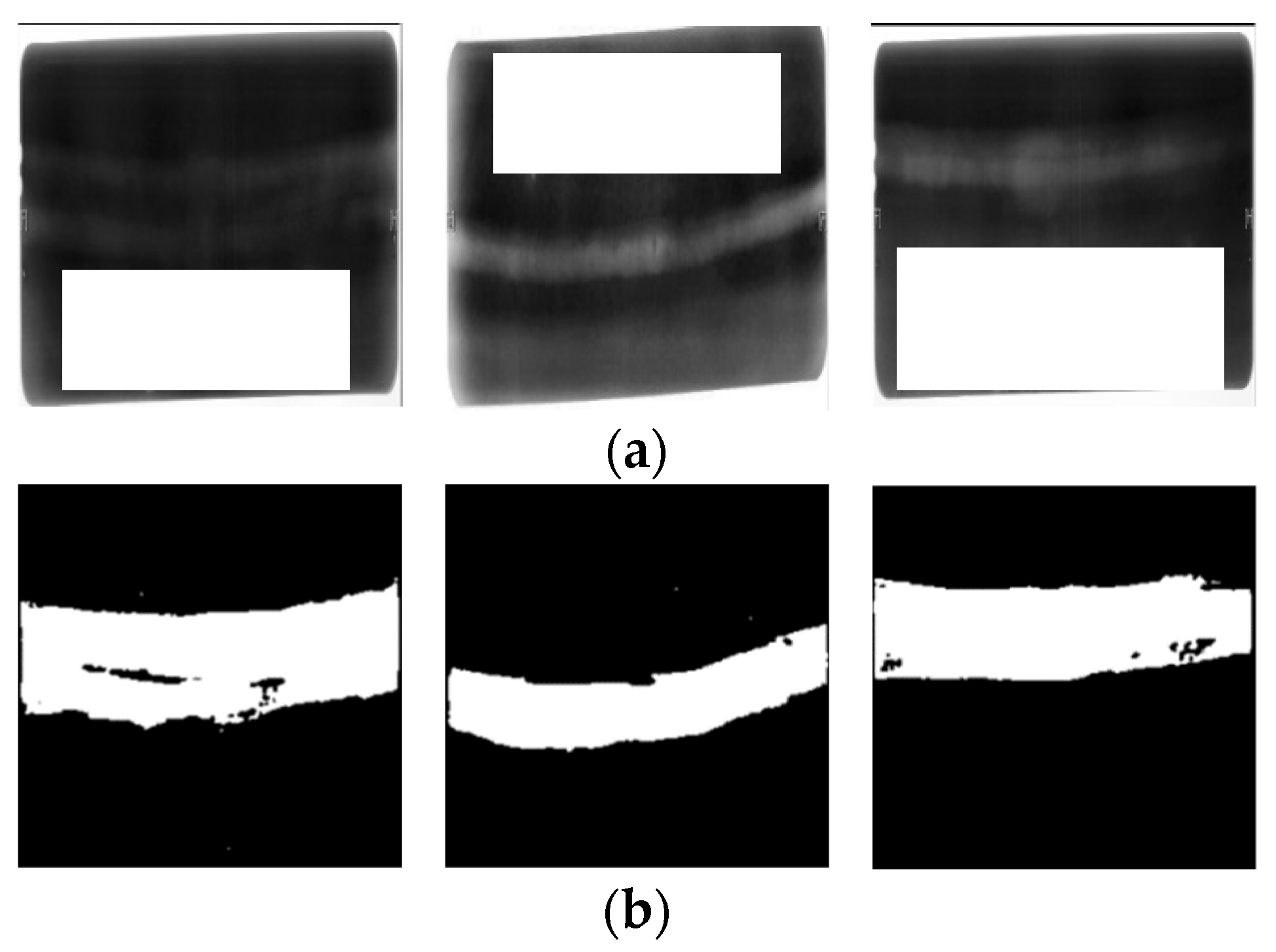
Figure 8 shows the predicted mask image results when only the weld images were input to the trained model without the mask images.
Figure 8a shows the image that was input to the trained model, and
Figure 8b shows the predicted shape and location of the bead in the input image.
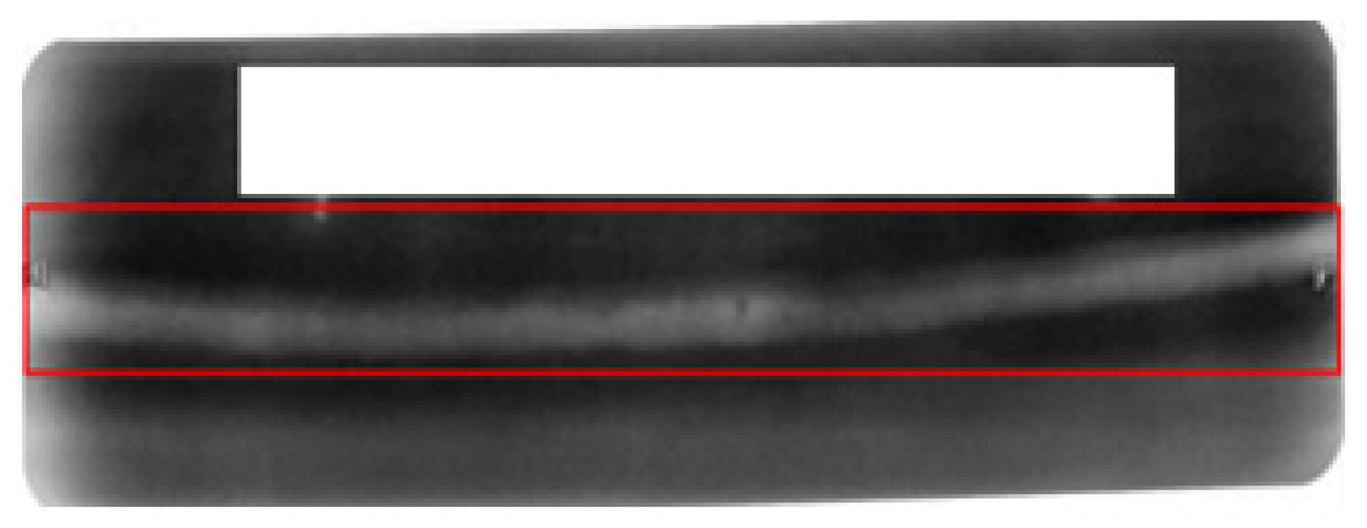
To extract only the weld bead from the predicted bead shape image as a post-processing operation, only the area with a pixel intensity of one was used; however, when detecting the bead, problems can occur owing to noise in the image. To resolve these problems, the algorithm shown in Algorithm 2 was used to find the largest area among the areas with a pixel intensity of one and perform a bounding box labeling operation on the weld image, as shown in
Figure 9. The coordinates of the four edges of the bounding box were determined, and the image was cropped to extract only the weld bead, as shown in
Figure 10.
| Algorithm 2. Algorithm for cropping image. |
| Input: Raw image, mask area coordinates:
|
|
|
| |
| Output: bead image
|
Calculate areas of : : min : max : min : max
|
- 2
Extract the largest area coordinates:
|
- 3
Draw bounding box in mask image: Rectangle
|
- 4
Cropping image: Bead image = Raw image
|
4.2. Results of Image Segmentation with Other Algorithms
The image segmentation method presented in this study was compared with other algorithms. Two algorithms were used for comparison. The first method is k-means clustering [
25]. The k-means algorithm is a clustering algorithm that divides given data into k regions. In the field of image segmentation, it refers to a process of dividing an image into several parts; that is, a set of pixels. The second method is image thresholding [
26], which is often used in image processing. Image thresholding is one of the simple methods of image segmentation, which distinguishes objects and backgrounds in an image and resets the pixel intensity with only two intensities. Two methods were performed on the same weld image as in
Figure 9.
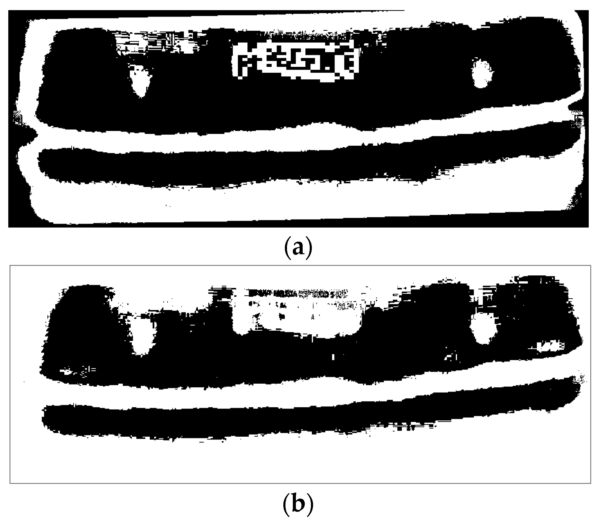
Figure 11 shows an image in which k-means algorithm is performed.
Figure 12 shows an image in which image thresholding is performed. When image segmentation was performed in two methods, it was difficult to extract only beads from the image. In the radiograph image, information of the image was also indicated in text form. The k-means and image thresholding methods determined the bead and text as the same area and segmented the image. Additionally, the border of the image was determined to be the same area as the bead. Accurate image segmentation was impossible because the contrast of the image varies depending on the light transmittance and a specific area may become too bright.
Figure 13a,b shows the binary images of
Figure 11 and
Figure 12, respectively. To evaluate the performance of the algorithms, binary images were compared with the true mask image set to obtain IoU, mIoU, and pixel accuracy.
Table 4 presents the performance evaluation results as average values for the image set. In
Table 4, (a) is the result of images in which k-means is performed, and (b) is the result of images in which thresholding is performed.
5. Conclusions
To efficiently inspect and determine defects and inadequate of the weld zone, a method of extracting only the weld bead from radiographic testing image was conducted.
The contrast of the weld image was improved using CLAHE as an image preprocessing operation, so that the weld zone became more prominent. Additionally, by performing data augmentation, 500 weld images were expanded to a total of 2500 images. The U-Net deep learning algorithm was used as an algorithm for extracting weld beads. After the training, the performance of the three models was compared.
The mIoU values for training and test data derived from model trained with images applied with CLAHE and data augmentation were 90.58% and 85.44%, respectively, and those for training and test data derived from model trained with images applied with only CLAHE were 89.93% and 84.88%, respectively. On the other hand, the mIoU values for training and test data derived from model with raw images were 89.10% and 83.47%, showing the lowest values. The deep learning performance was improved by applying CLAHE and data augmentation.
In the radiographic testing images, information about the image as well as weld bead was marked. Additionally, although the proportion of weld bead in the image is not large, the weld bead could be effectively extracted as a result of image post-processing based on the trained results.
The method presented in this study was compared with the results of general image segmentation methods. Since general image segmentation methods determined that beads and text were the same area in the image, it was difficult to extract only beads. In contrast, it was confirmed that U-Net could extract only beads from images and produced better results than other image segmentation methods.
Five hundred radiographic testing images were used in the experiment, and a higher degree of accuracy for a wider variety of weld image types can be achieved by procuring additional images in the future. Additionally, it will be possible to reduce the time and cost of the weld quality inspections by automating the extraction of the weld bead shapes.
Author Contributions
Conceptualization, G.-s.J., S.-j.O., Y.-s.L. and S.-c.S.; methodology, G.-s.J., S.-j.O., Y.-s.L. and S.-c.S.; validation, G.-s.J., S.-j.O., Y.-s.L. and S.-c.S.; formal analysis, G.-s.J., Y.-s.L. and S.-c.S.; investigation, G.-s.J. and S.-j.O.; writing—original draft preparation, G.-s.J.; writing—review and editing, G.-s.J. and S.-j.O.; supervision, Y.-s.L. and S.-c.S.; project administration, Y.-s.L. and S.-c.S. All authors have read and agreed to the published version of the manuscript.
Funding
This research received no external funding.
Institutional Review Board Statement
Not applicable.
Informed Consent Statement
Not applicable.
Data Availability Statement
Not applicable.
Acknowledgments
This paper was written with the support of the Korea Institute for Advancement of Technology funded by the Ministry of Trade and Industry in 2021, the “Autonomous Ship Technology Development Project (20200615)”.
Conflicts of Interest
The authors declare no conflict of interest.
References
- Kim, Y.; Kil, S. Latest Technology of Non Destructive Inspection for Welded Structure. J. Weld. Join. 2017, 35, 63–70. [Google Scholar] [CrossRef]
- Lee, S.B. Trend of Nondestructive Testing in Shipbuilding Industry. J. Weld. Join. 2010, 28, 5–8. [Google Scholar] [CrossRef][Green Version]
- Mahmoudi, A.; Regragui, F. Welding defect detection by segmentation of radiographic images. In Proceedings of the 2009 WRI World Congress on Computer Science and Information Engineering, Los Angeles, CA, USA, 31 March–2 April 2009; pp. 111–115. [Google Scholar]
- Mahmoudi, A.; Regragui, F. Fast segmentation method for defects detection in radiographic images of welds. In Proceedings of the 2009 IEEE/ACS International Conference on Computer Systems and Applications, Rabat, Morocco, 10–13 May 2009; pp. 857–860. [Google Scholar]
- Vilar, R.; Zapata, J.; Ruiz, R. An automatic system of classification of weld defects in radiographic images. NDT E Int. 2009, 42, 467–476. [Google Scholar] [CrossRef]
- Jiang, H.; Zhao, Y.; Gao, J.; Wang, Z. Weld extraction of radiographic images based on Bezier curve fitting and medial axis transformation. Insight-Non-Destr. Test. Cond. Monit. 2016, 58, 531–535. [Google Scholar] [CrossRef]
- Jiang, H.; Li, H.; Yang, L.; Wang, P.; Hu, Q.; Wu, X. A fast weld region segmentation method with noise removal. In Proceedings of the 2019 IEEE 4th Advanced Information Technology, Electronic and Automation Control Conference (IAEAC), Chengdu, China, 20–22 December 2019; Volume 1, pp. 1492–1496. [Google Scholar]
- Ronneberger, O.; Fischer, P.; Brox, T. U-net: Convolutional networks for biomedical image segmentation. In Proceedings of the International Conference on Medical Image Computing and Computer-Assisted Intervention, Munich, Germany, 5–9 October 2015; Springer: Cham, Germany, 2015; pp. 234–241. [Google Scholar]
- Reza, A.M. Realization of the contrast limited adaptive histogram equalization (CLAHE) for real-time image enhancement. J. VLSI Signal Process. Syst. Signal Image Video Technol. 2004, 38, 35–44. [Google Scholar] [CrossRef]
- Shorten, C.; Khoshgoftaar, T.M. A survey on image data Augmentation for deep learning. J. Big Data 2019, 6, 60. [Google Scholar] [CrossRef]
- Rukundo, O. Effects of Image Size on Deep Learning. arXiv 2021, arXiv:2101.11508. [Google Scholar]
- Kang, S.J.; Han, D.S. A Robust Road Sign Information Detection Method in Dark and Noisy Scene Using CLAHE. In Proceedings of the Korean Society of Broadcast Engineers Conference, Jeju, Korea, 29 June–1 July 2016; The Korean Institute of Broadcast and Media Engineers: Seoul, Korea, 2016; pp. 361–363. [Google Scholar]
- Perez, L.; Wang, J. The effectiveness of data Augmentation in image classification using deep learning. arXiv 2017, arXiv:1712.04621. [Google Scholar]
- Kaymak, Ç.; Uçar, A. A brief survey and an application of semantic image segmentation for autonomous driving. In Handbook of Deep Learning Applications; Springer: Cham, Germany, 2019; pp. 161–200. [Google Scholar]
- Long, J.; Shelhamer, E.; Darrell, T. Fully convolutional networks for semantic segmentation. In Proceedings of the IEEE Conference on Computer Vision and Pattern Recognition, Boston, MA, USA, 7–12 June 2015; pp. 3431–3440. [Google Scholar]
- Oh, Y.T.; Park, H.J. Multi-resolution U-Net for segmentation of lung CT scan. In Proceedings of the Institute of Electronics and Information Engineers Autumn Conference, Gwangju, Korea, 27–28 December 2020; pp. 652–655. [Google Scholar]
- Albawi, S.; Mohammed, T.A.; Al-Zawi, S. Understanding of a convolutional neural network. In Proceedings of the 2017 International Conference on Engineering and Technology (ICET), Antalya, Turkey, 21–23 August 2017; pp. 1–6. [Google Scholar]
- Wan, F. Deep Learning Method Used in Skin Lesions Segmentation and Classification; KTH Royal Institute of Technology: Stockholm, Sweden, 2018. [Google Scholar]
- Brownlee, J. Train-Test Split for Evaluating Machine Learning Algorithms. 2020. Available online: https://machinelearningmastery.com/train-test-split-for-evaluating-machine-learning-algorithms/ (accessed on 9 September 2021).
- Hayou, S.; Doucet, A.; Rousseau, J. On the Impact of the Activation Function on Deep Neural Networks Training. In Proceedings of the International Conference on Machine Learning (PMLR), Long Beach, CA, USA, 9–15 June 2019; pp. 2672–2680. [Google Scholar]
- Ruby, U.; Yendapalli, V. Binary cross entropy with deep learning technique for image classification. Int. J. Adv. Trends Comput. Sci. Eng. 2020, 9, 5393–5397. [Google Scholar]
- Zhang, Z. Improved adam optimizer for deep neural networks. In Proceedings of the 2018 IEEE/ACM 26th International Symposium on Quality of Service (IWQoS), Banff, AB, Canada, 4–6 June 2018; pp. 1–2. [Google Scholar]
- Jordan, J. Evaluating Image Segmentation Models. 2018. Available online: https://www.jeremyjordan.me/evaluating-image-segmentation-models/ (accessed on 9 September 2021).
- Everingham, M.; Van Gool, L.; Williams, C.K.; Winn, J.; Zisserman, A. The pascal visual object classes (voc) challenge. Int. J. Comput. Vis. 2010, 88, 303–338. [Google Scholar] [CrossRef]
- Dhanachandra, N.; Manglem, K.; Chanu, Y.J. Image segmentation using K-means clustering algorithm and subtractive clustering algorithm. Procedia Comput. Sci. 2015, 54, 764–771. [Google Scholar] [CrossRef]
- Sahoo, P.K.; Soltani, S.A.K.C.; Wong, A.K. A survey of thresholding techniques. Comput. Vis. Graph. Image Process. 1988, 41, 233–260. [Google Scholar] [CrossRef]
Figure 1.
The redistribution will push some pixels over the clip limit again (region shaded green in the figure). It can be left as it is, but if this is undesirable, the redistribution procedure can be repeated recursively until the excess is negligible.
Figure 1.
The redistribution will push some pixels over the clip limit again (region shaded green in the figure). It can be left as it is, but if this is undesirable, the redistribution procedure can be repeated recursively until the excess is negligible.
Figure 2.
U-Net architecture.
Figure 2.
U-Net architecture.
Figure 3.
An average of 33 differences were present in the pixels in the bead area before and after HE was applied: (a) raw image; (b) CLAHE image.
Figure 3.
An average of 33 differences were present in the pixels in the bead area before and after HE was applied: (a) raw image; (b) CLAHE image.
Figure 4.
Pixel distribution of the image was broadened through HE: (a) histogram for the raw image; (b) histogram for the CLAHE image.
Figure 4.
Pixel distribution of the image was broadened through HE: (a) histogram for the raw image; (b) histogram for the CLAHE image.
Figure 5.
Mask image consisting of pixel intensity 0 of basic metal and 1 of weld bead.
Figure 5.
Mask image consisting of pixel intensity 0 of basic metal and 1 of weld bead.
Figure 6.
Results of the testing of 2500 images model in which CLAHE and data augmentation are performed: (a) input images; (b) true mask images; (c) predicted mask images.
Figure 6.
Results of the testing of 2500 images model in which CLAHE and data augmentation are performed: (a) input images; (b) true mask images; (c) predicted mask images.
Figure 7.
Loss function in training and testing: (a) 500 raw images model; (b) 500 images model in which CLAEH is performed; (c) 2500 images model in which CLAHE and data augmentation are performed.
Figure 7.
Loss function in training and testing: (a) 500 raw images model; (b) 500 images model in which CLAEH is performed; (c) 2500 images model in which CLAHE and data augmentation are performed.
Figure 8.
Results of entering only weld images in 2500 images model in which CLAHE and data augmentation are performed: (a) input images; (b) predicted mask images.
Figure 8.
Results of entering only weld images in 2500 images model in which CLAHE and data augmentation are performed: (a) input images; (b) predicted mask images.
Figure 9.
Bounding box image drawn along the bead shape.
Figure 9.
Bounding box image drawn along the bead shape.
Figure 10.
Results of the experiment.
Figure 10.
Results of the experiment.
Figure 11.
An image in which k-means is performed.
Figure 11.
An image in which k-means is performed.
Figure 12.
An image in which image thresholding is performed.
Figure 12.
An image in which image thresholding is performed.
Figure 13.
Binary images: (a) binary image of image in which k-means is performed; (b) binary image of image in which thresholding is performed.
Figure 13.
Binary images: (a) binary image of image in which k-means is performed; (b) binary image of image in which thresholding is performed.
Table 1.
Experimental environment.
Table 1.
Experimental environment.
| | Value |
|---|
| OS | Window 10 64 bit |
| CPU | Intel(R) Core(TM) i7-8700k@3.70 GHz |
| RAN | 32 GB |
| GPU | NVIDIA TITAN Xp |
Table 2.
Confusion matrix.
Table 2.
Confusion matrix.
| | Predicted Positive | Predicted Negative |
|---|
| Actually Positive | True positive (TP) | False negative (FN) |
| Actually Negative | False positive (FP) | True negative (TN) |
Table 3.
Results of experiment: (a) the result of 500 raw images; (b) the result of 500 images in which CLAHE is performed; (c) the result of 2500 images in which CLAHE and data augmentation are performed.
Table 3.
Results of experiment: (a) the result of 500 raw images; (b) the result of 500 images in which CLAHE is performed; (c) the result of 2500 images in which CLAHE and data augmentation are performed.
| | | IoU | mIoU | Accuracy |
|---|
| (a) | Train | 83.00% | 89.10% | 97.48% |
| Test | 73.58% | 83.47% | 95.53% |
| (b) | Train | 83.24% | 89.93% | 97.58% |
| Test | 75.01% | 84.88% | 95.61% |
| (c) | Train | 83.78% | 90.58% | 98.01% |
| Test | 76.01% | 85.44% | 95.90% |
Table 4.
Results of comparing with the true mask image set: (a) the result of images in which k-means is performed; (b) the result of images in which thresholding is performed.
Table 4.
Results of comparing with the true mask image set: (a) the result of images in which k-means is performed; (b) the result of images in which thresholding is performed.
| | IoU | mIoU | Accuracy |
|---|
| (a) | 20.06% | 40.22% | 44.18% |
| (b) | 18.34% | 29.93% | 38.72% |
| Publisher’s Note: MDPI stays neutral with regard to jurisdictional claims in published maps and institutional affiliations. |
© 2021 by the authors. Licensee MDPI, Basel, Switzerland. This article is an open access article distributed under the terms and conditions of the Creative Commons Attribution (CC BY) license (https://creativecommons.org/licenses/by/4.0/).


