Abstract
The water in the rock medium is exchanged with the confined aquifer through the fracture, which leads to the water inflow line in the confined aquifer is no longer horizontal. This paper assumes that the aquifuge is a kind of semi-isolation layer, while the first-order derivative of the total head slope line function within the influence of precipitation approaches the slope of the line connecting the top plate of the aquifuge with the spherical center. This hypothesis demonstrates the relationship between the bottom of the well water inflow and the complete well gushing water. Laplace’s equation for the spherical coordinate transformation is used to find the analytical solution of the water inflow for stable flow. The calculation results are in line with reality through actual engineering and numerical simulation methods. The current numerical simulation methods and theoretical methods mostly consider the aquifer in the ideal state, which is difficult to simulate the fractured rock mass. The theoretical formula proposed in this paper can more effectively reflect the actual seepage situation of fractured rock mass than other formulas. In addition, the combination of theoretical derivation, numerical simulation and field measurement can predict the water inflow more accurately than unilateral research. At the same time, for the question of whether the face excavation is grouted or not, this paper using the subjective and objective assignment weight method combined with analytic hierarchy process method and entropy-weight method to take the weight calculation and giving a slurry excavation judgment method based on the proposed formula. Theoretical support is given for the selection of permeability coefficients for each hole in the overrun exploration and this method is validated by different projects, which has some degree of reference value.
1. Introduction
In the construction of water-rich areas, whether in tunnels or shafts, water gushing is always the most difficult problem to deal with, and accidents such as sudden flooding of tunnels and shaft flooding occur frequently, causing great damage to property and casualties. In the construction of water-rich areas, whether in tunnels or shafts, water gushing is always the most difficult problem to deal with, and accidents such as sudden flooding of tunnels and shaft flooding occur frequently, causing great damage to property and casualties. Generally, the number of over-bored holes is one. However, the parameters of each hole are not the same in the actual rock project. Therefore, how to choose a suitable parameter about the grouting judgment is a very important issue. When excavating the aquifer, if only the ideal geological conditions are considered, there may be a large error in the prediction of water inflow. When the predicted value is small, the excavation without grouting may exceed the drainage capacity of the shaft and cause flooding. Therefore, there is an urgent need to develop mathematical models for different geologies and to form a grouting judgment system in combination with advance exploration to prevent accidents and ensure the safety of the project.
Now there are many methods of predicting influx of water, including precipitation infiltration method, subsurface runoff modulus method, groundwater dynamics method, comparison method, fuzzy mathematical method, numerical simulation method, etc. On the groundwater dynamics method in the normal influx of stable flow problems, Dupuit based on Darcy’s law proposed Dupuit hypothesis. People based on the assumption of semi-infinite aquifer, improve the ground water head above the surface of the horizontal tunnel steady-state flow, transient flow of water prediction formulae and the ground water head below the surface of the water inlet formula [1,2,3,4,5]. Furthermore, some people proposed their own equations based on different mathematical models [6,7,8,9,10,11,12,13,14,15,16,17]. However, all of them have some errors or are incomplete. For example, the formula of Luo ignores the water inlet at the top of the cave when the water level is higher than the surface [15,16], while the rest of the formulas all ignore the water surge at the palm surface. A number of Chinese scholars improved the previous formulas to some extent based on mathematical methods such as angle-preserving mapping and mirroring method [18,19,20,21,22,23]. Although now has proposed a lot of water surge analytical formula, but all of them are based on different mathematical simplification model proposed. These formulas are more suitable for isotropic geological excavation, but there are still few formulas suitable for fractured rock mass such as anisotropic medium excavation. In addition, double porosity is not considered in many formulas.
With the development of calculation technology, various numerical simulation software have high accuracy in water inflow prediction. Among the available studies, COMSOL Multiphysics [24,25], FLAC3D [26,27,28,29] and MODFLOW [30,31,32] and other software verified to be better able to simulate the engineering water surges in excavations under complex geological conditions. Therefore, the analysis of the water surge in recent years has focused on numerical means of research, and less research on theoretical aspects. Although the numerical simulation method can take into account the actual situation of the project, including geology, excavation profile, flow-solid coupling, etc., to some extent, it has its own limitations. As stated by Hwang and Lu [33] numerical model are tedious, time-consuming, and expensive for tunnel engineers in practice. For example, their assumptions are mostly small deformations and have great reliance on the ground investigation data. Due to the accuracy and difficulty of actual exploration, it makes the model parameters have certain errors, which may produce simulation results that are not in line with reality in some projects.
Therefore, this paper takes theoretical analysis, numerical simulation, field measurements methods to predict the water inflow of Gaoligong Mountain. Propose a new formula for predicting water influx, considering the non-horizontal flow of the aquifer, while combining numerical simulation results and actual measurement results for error analysis. In addition, for the palm face grouting problem, this paper based on the proposed formula to calculate the weight value of the permeability coefficient of different hole backcalculation of over exploration and verification, forming a set of grouting excavation judgment method.
2. Formula Derivation
Basic assumptions.
- (1)
- The rock formation is a homogeneous porous medium;
- (2)
- The permeability coefficient of the formation is the same in all directions;
- (3)
- The flow is steady flow;
- (4)
- The radius of influence is considered to be twice the distance from the stationary water surface to the bottom of the well according to Japanese data [34];
- (5)
- The primary derivative of the full head slope drop curve within the precipitation influence area approximates the slope of the line connecting the top plate of the water barrier to the center of the sphere.
The conservation of mass and the continuity equation gives,
while the schematic diagram is shown in Figure 1. Introducing Darcy’s law, i.e.,
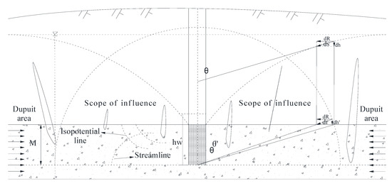
Figure 1.
Mathematical model schematic.
A spherical coordinate representation is used to Equation (2),
The seepage field of the shaft excavation is symmetric about the Z-axis, i.e.,
Taking , separate the variables twice to obtain,
Taking , Equation (5) can be transformed into Legendre’s equation as follows,
Then the general solution of H is,
The following two equations hold in the influence range and outside the influence range,
The boundary condition is,
Due to , the aquifer is less affected by pumping when is large, and the flow line is basically horizontal. Meanwhile, is established and is the flow rate per extended meter of well. Therefore,
Equation (9) is divided by around, i.e.,
The right side of Equation (10) tends to 0 and the first term on the left tends to 0. However, there exist infinite values of the remaining terms, and the orders are all different. So, if both sides of Equation (10) converge to 0, it needs to have,
i.e.,
In the influence range, when is small, is tends to 0. Therefore, is constant, i.e.,
In this paper, we assume that the radius of influence of precipitation is , while there are and for sphere. We can obtain,
i.e.,
We can derive,
Therefore, the total head general solution is,
Since the full head is equal to the sum of position head, pressure head, velocity head. We can derive the relationship between the coefficients as follows,
The slope of the gradient curve of the confined intact well is , while the slope of bottom of confined well is . We can find there are an relationship between and , where is the slop of the line between the top plate of confined aquifer and the center of the sphere. So, we assume that the slope of the semi-infinite confined aquifer gradient curve is approximately equal to the slope of the spherical core line when the head slope tends to 0, i.e., . Equation (18) can be transformed into,
Separating the variables and using the boundary conditions yields, we can acquire,
Since the position head and velocity head of the steady flow are the same, the Equation (20) is equal to,
And the water inflow of confined complete well is,
where is thickness of confined aquifer, is permeability coefficient, is excavation radius, is the total head, is the water inflow at , is the influent radius, is height in well, is the density of water, and is the gravitational acceleration. The following is the derivation of the water inflow formula for grouting. If the water pressure at the inner diameter of the liner is considered to be 0, the water pressure at the outer diameter of the liner is . The water pressure at the radius of the grouting circle is , and the water pressure at the radius of the grouting circle is . The permeability coefficients of the liner, grout layer, and rock are . Therefore, the following equation holds.
Lining
Grouting ring
Lithosphere
Combining Equations (23)–(25), we are able to obtain,
There are for grouting excavation. Therefore, Equation (26) has the following forms,
Combining Equation (22) with the dupuit formula of phreatic, we can acquire,
And we are able to derive confined—phreatic stable flow of water inflow formula,
where is the radius when the total head is equal to the thickness of confined aquifer, the others contents are same to above.
Similarly, we can acquire the formula of grouting,
where is the radius of grouting ring, and the others contents are same to above.
3. Analysis of the Water Inflow in the Main Shaft of Gaoligong Mountain No. 1 Shaft
Gaoligong Mountain No. 1 Shaft construction is under high water pressure. In order to ensure the safe construction of the project, there is need to grout when having water. Therefore, the actual measured water inflow data is the data after the slurry injection and the data of no grouting is unknow. We use the numerical simulation method to acquire the data of no grouting. For the characteristics of steeply tilted large fracture in Gaoligong Mountain No. 1 Shaft construction, a narrow double void media model is used for simulation.
The built-in DFN plug-in function of FLAC3D is used to realize solid random fracture medium modeling, while the pore medium is simulated by solid unit.
3.1. Engineering Background
The Gaoligong Mountain is located between Nujiang and Longling stations, with a maximum burial depth of about 1155 m. The tunnel inlet mileage is D1K192 + 302, the exit mileage is D1K226 + 840, the total length of the tunnel is 34,538 m. In order to speed up the construction progress and solve the problems of construction ventilation and operation ventilation, No. 1 shaft is set up in the middle of the cave. No. 1 shaft sub-shaft is located 52 m to the left of D1K205 + 053 line, and the depth of shaft is 764.74, just like Figure 2.
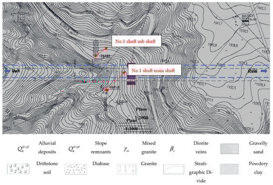
Figure 2.
Topographic plan of shaft No. 1.
3.2. Stratigraphic Lithology and Hydrogeology
According to the drill hole BPDZ-22-01 drilling revealed, the corresponding cores are show in Figure 3. The lithology of the strata traversed by the shaft are shown in Table 1.
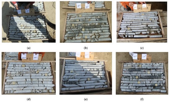
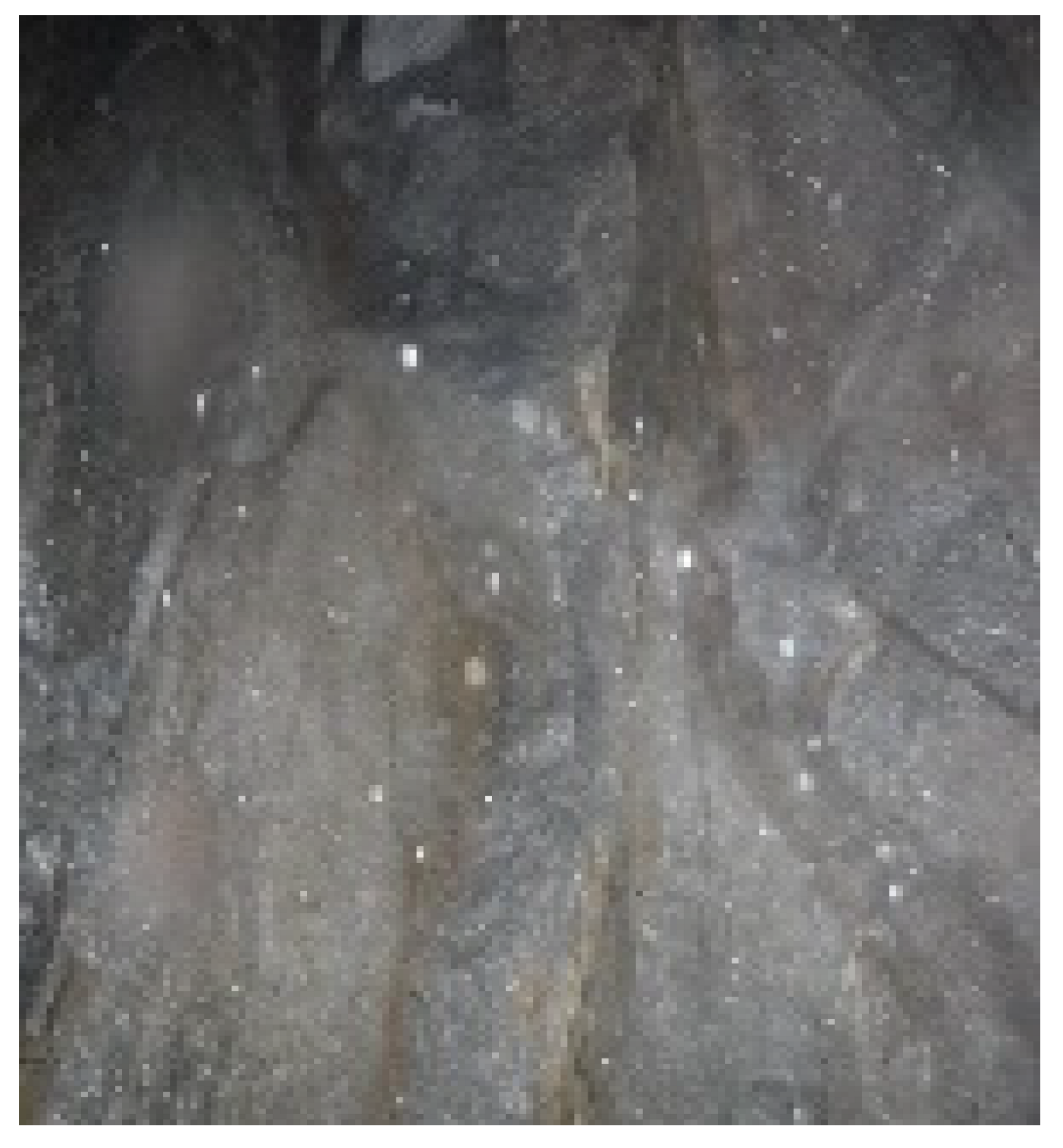
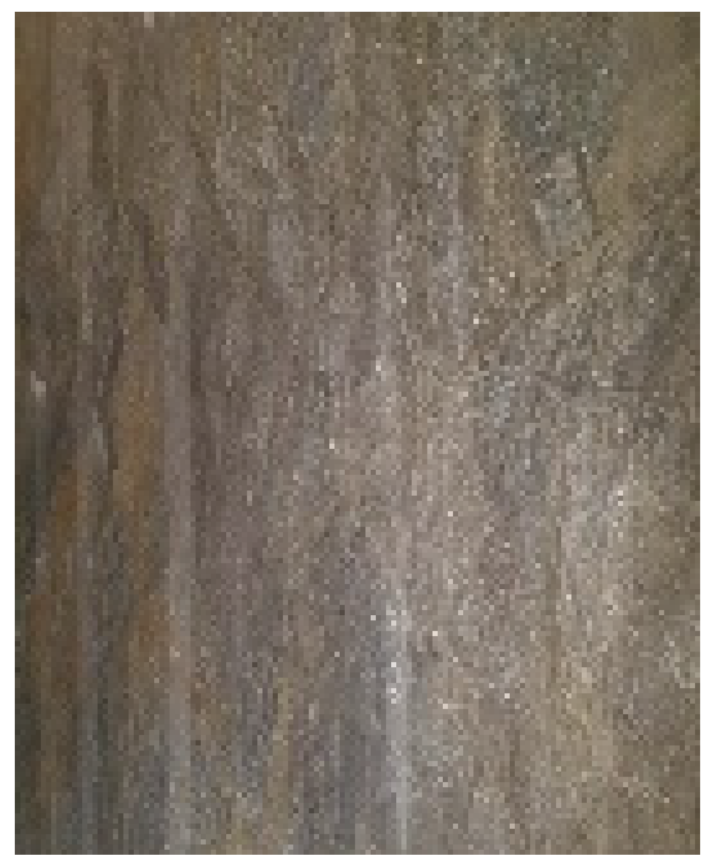
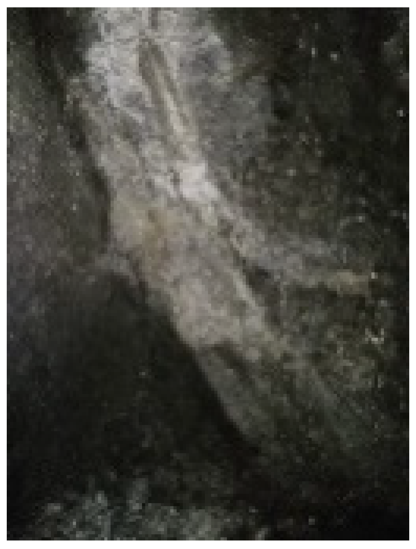
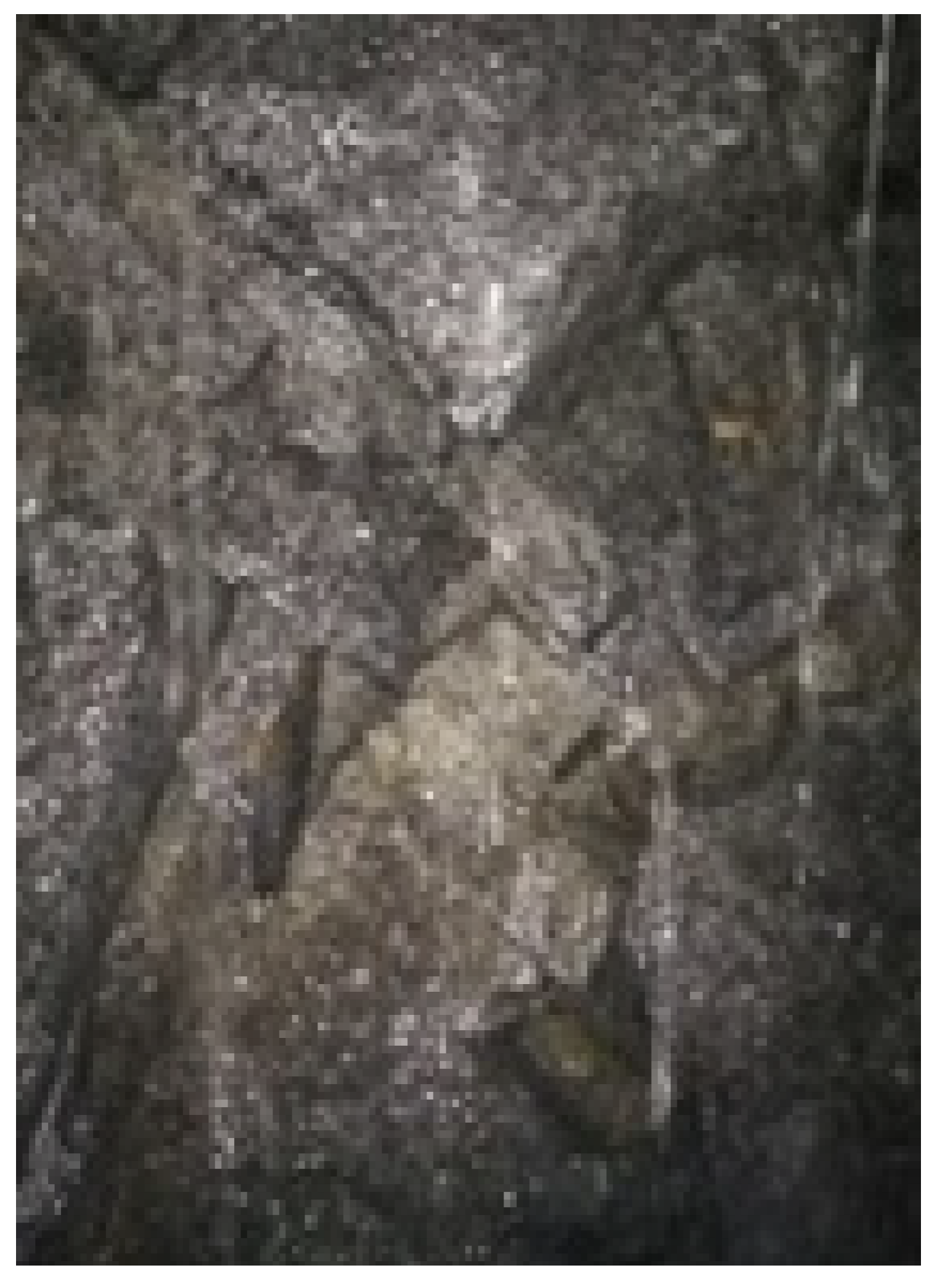
Figure 3.
Core images of No. 1 shaft sub shaft. (a) 101.3 to 114.0 m; (b) 269.10 to 280.50 m; (c) 380.60 to 391.70 m; (d) 456.10 to 466.00 m; (e) 601.30 to 611.50 m; (f) 666.80 to 678.70 m.

Table 1.
Lithology of strata at different depths.
The groundwater of No. 1 shaft is mainly pore water and bedrock fracture water of the fourth system loose rock type, the main aquifer is granite with fracture development. The pore water is mainly pore water in the surface powder clay and fully weathered granite layer. According to the borehole, the wellbore traverses four confined aquifers, and the permeability coefficient is back-calculated by dupuit single-hole stable flow formula. The hydrological parameters are shown in Table 2.
Table 2.
Hydrogeological parameters.
According to the grouting water pressure test of Gaoligong Mountain, the water head of Gaoligong Mountain is very high, as shown in Figure 4. In Figure 4b, the steep crack at 630 m is developed, and the grouting effect is poor. Therefore, several times of grouting have been carried out, which leads to the water pressure obtained at this time belongs to the water pressure after grouting. In addition, this is the reason why water pressure dropped fast at A. The water heads at different depths are basically equal to, regardless of the main shaft or auxiliary shaft.
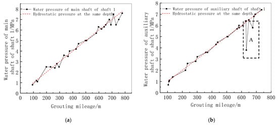
Figure 4.
Measured water pressure of No. 1 and No. 2 shafts in Gaoligong Mountains. (a) Water pressure of main shaft of shaft 1; (b) Water pressure of auxiliary shaft of shaft 1.
3.3. Numerical Simulation
This paper adopts the narrow double void medium theory that assumes rock is composed of fractured medium and pore medium to consider that the steeply dipping large fractured rock masses in the Gaoligong Mountains. Two different hydrological parameters are assigned to model. Both media are simulated by solid units. The gross hole radius of the shaft is 3 m, the lining thickness is 0.45 m, the excavation depth is about 770 m, and the grouting range is 9 m. Since the project size is too large, the layers of four aquifers are used for analysis. Therefore, the model size is taken as 160 m × 160 m × 66 m.
The radius of excavation is 3 m, the thickness of lining is 0.5 m, another 0.1 m thickness of ground stress release area is taken, and the thickness of grouting ring is 4 m. Combined with the field fracture survey data, the statistical parameters of different fracture groups are shown in Table 3. The fractured solid network generated by the random discrete fracture network generation plug-in of FLAC3D is displayed in Figure 5.
Table 3.
In-situ fracture survey data for different fracture groups.
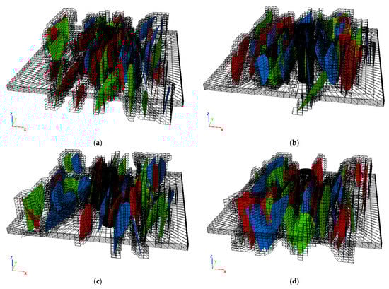
Figure 5.
Discrete fracture networks and aquifers. (a) Aq1, (b) Aq2, (c) Aq3, (d) Aq4.
The geology of Gaoligong Mountain revealed by the overrun borehole is mainly granite geology with different degrees of weathering and fracture filling. Therefore, the geological parameters and hydrological parameters of the model are simplified as Table 4. It is considered that the mechanical parameters decrease by 1 order of magnitude and the permeability parameters increase by 3 order of magnitude for the parameters of the fractured medium. After grouting, the rock strength increases by one order of magnitude and the permeability coefficient is calculated inversely through the water inflow of the inspection hole of the working face. The surrounding boundary of aquifer is a permeable boundary, and the other area is considered impermeable considering the delayed water release characteristics of the rock. The model boundary is the replenishment boundary, which fixes the displacement of each surface.
Table 4.
Model total geological parameters at different depths.
The initial pore pressure field is displayed in Figure 6a,b. When not disturbed by excavation, the water pressure in rock mass is basically equal to . We can see that in addition to solitary fractures, there are many steep large fractures penetrating the aquifer. As for why the water pressure in Gaoligong Mountain is so large, some people think that there is high pressure fracture water in the solitary fracture. This paper believes that the small fracture runs through the steep large fracture, and the steep large fracture runs through the aquifer, so that the total head in the fracture is the same as that in the aquifer. Only in this way can we explain why the total water inflow in the whole period of shaft construction has not been reduced.
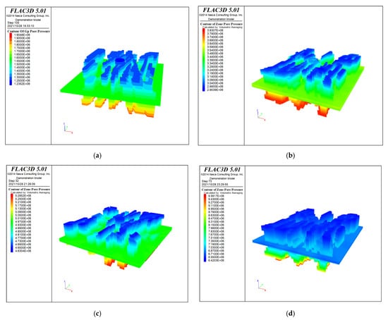
Figure 6.
The initial pore pressure field of fracture network. (a) Aq1, (b) Aq2, (c) Aq3, (d) Aq4.
3.4. Water Inflow Analysis
The site shaft excavation is 3.6 m per section, while this paper takes the simulation of four confined aquifer excavation to the bottom. No grouting excavation and grouting excavation under the four processes at the seepage field changes are shown in Figure 7 and Figure 8. Meanwhile, taking the FISH language programming to derive the shaft the water inflow.
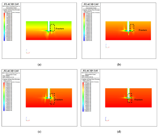
Figure 7.
Hydraulic pressure field of different excavation sections without grouting. (a) Aq1, (b) Aq2, (c) Aq3, (d) Aq4.
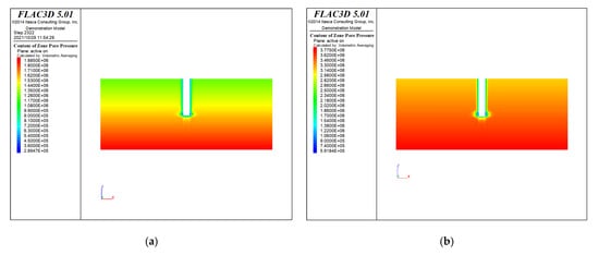
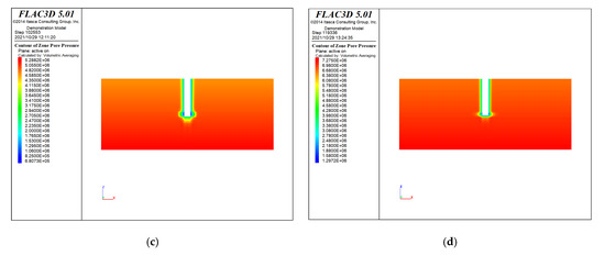
Figure 8.
Hydraulic pressure field of different excavation sections with grouting. (a) Aq1, (b) Aq2, (c) Aq3, (d) Aq4.
Figure 7 and Figure 8 show the water pressure nephogram under non grouting excavation and grouting excavation, respectively. We can see that under the influence of drainage, fissure water will flow through the fractures and supplement the confined water layer. Then, the rock pore water replenishes the fissure water, and replenishes the confined water layer through the fissure. Therefore, when analyzing fractured rock mass, we should consider the influence of rock water replenishment through fractures, rather than using the ideal circular island model simply.
According to the site construction palm surface inspection hole disclosure, the permeability coefficient mean value of each grouted hole is shown in Table 5. As for the reason that taking the mean value will be discussed as following. Next, the dupuit formula and the improved formula proposed by this paper are applied to the prediction of water inflow.
Table 5.
Permeability coefficient values for different aquifers with grouting of No. 1 Shaft.
The calculation results are shown in Table 6. Where Q1 stands for the water inflow for the dupuit formula of no grouting, Q2 represents the actual measured water inflow, Q3 is water inflow for no grouting of the improving formula this paper puts forward, Q4 is water grouting inflow using the improving formula which will shown in forward paper, Q5 is the result of numerical simulation of excavation without grouting, and Q6 is the result of numerical simulation of excavation grouting.
Table 6.
Comparison of predicted values of different formulas of water inflow.
As it can be seen from Table 6, the grouting simulation results are close to the measured values, larger than the original pressure-bearing to pressure-free formula. The measured data is the water inflow after blasting excavation. When the water inflow is large, secondary grouting measures was taken. The results of the grout-free simulation are much larger than the original pressure-bearing to pressure-free equation and are closer to the predicted results of grout-free excavation in this paper with small permeability coefficient. The formula calculation results of both grouting formula this paper proposed and the original pressure-bearing to pressure-free formula all close to the actual measurement and numerical simulation results. However, the permeability coefficient of the original pressure-bearing to pressure-free formula is no grouting, which means the predicted value of water surge has great error.
4. A New Grouting Evaluation Method
Based on the previous proposed formula for predicting the water inflow, firstly, the different permeability coefficients obtained from the over-exploration workface are selected. Secondly, predict excavation of the total water inflow generated by the different feeds, and compare with drainage capacity of engineering. Finally, consider the possibility of using no grout excavation, the logic diagram is shown in Figure 9.
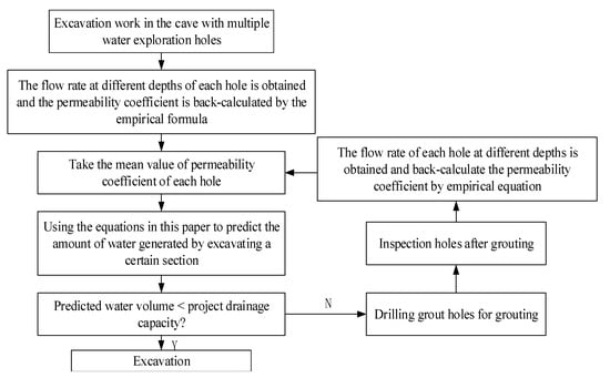
Figure 9.
Working face grouting excavation judgment method.
4.1. Total Water Inflow Prediction Formula
Shaft gushing water comes from well wall most. Therefore, the Grouting excavation total water inflow prediction formula is,
Correspondingly, no grouting excavation total water inflow prediction formula is,
where stand for excavation depth, while the others contents is the same as above. is not related to the excavation feed and take as for tunnel excavation.
4.2. Calculation of Permeability Coefficient Weights Based on the Equations in This Paper
In the existing literature, engineering and research are separated. In the research, we usually think that the permeability coefficient is a fixed value and ignore how it comes from engineering. In engineering, we usually think that when the dispersion of permeability coefficient is small, the mean or minimum value is used for calculation. It seems that we don’t know how to choose the value of permeability coefficient. We instinctively think that the more uniform the coefficient, the better, the smaller the coefficient, and the lower the cost, but how to show it theoretically is a problem, which is the reason why we carry out this problem analysis.
We use the following formula for the in-cave pressure water test here to calculate the permeability coefficient,
where is the water absorption per unit of stratum, is length of water injection or slurry section, is the radius of the water or slurry injection hole, stands for stable flow rate of water or slurry injection holes, and represents water or slurry injection pressure. Generally, the number of over-bored holes is one. However, the parameters of each hole are not the same in the actual rock project. Therefore, how to choose a suitable. parameter about the grouting judgment is a very important issue. For deep buried water-rich tunnels, the water pressure at tunnel top and invert is equal and can be basically treated as a complete well, and then Equation (29) is applicable.
Calculation of the coefficient of permeability using Equation (33) in the context of the Qiyue Mountain Tunnel and its specific weight to Equation (33) are shown below. The data of Qiyue Mountain Tunnel and Gaoligong Mountain No. 1 shaft main shaft were used to verify the accuracy of the calculation. Analytic Hierarchy Process method (APH) was used for calculating the subjective weights, the entropy weight method was used to calculate the objective weights, and the combined subjective and objective assignment weights were used to calculate the combined weights.
4.2.1. Analytic Hierarchy Process
APH model calculations such as Figure 10. In this study, the target layer is how to choose the permeability coefficient value based on the equations in this paper. Suppose the number of grouting inspection holes is and . Combined with the site, we choose five values as follows,
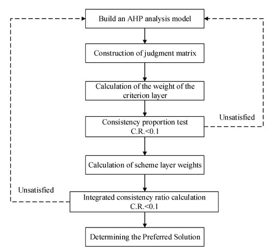
Figure 10.
Calculation process of AHP.
Therefore, the criterion layer is,
The program layer is,
Figure 11 stand for the indicator system. We consulted with domain experts through questionnaires, emails, etc., and scored them using the 9-point scale. Meanwhile, the construction of the judgment matrix is shown in Table 7, Table 8 and Table 9. At present, the methods after expert consultation mainly include sample average and weight average. When a large number of samples are counted, there will be a certain error when using sample average according to the existing research literature. At this time, weighted average should be used. However, in this study, because there are few consulting samples, and the consulting experts have more consistent answers. Therefore, we believe that it is satisfactory to calculate the weight after averaging the samples.
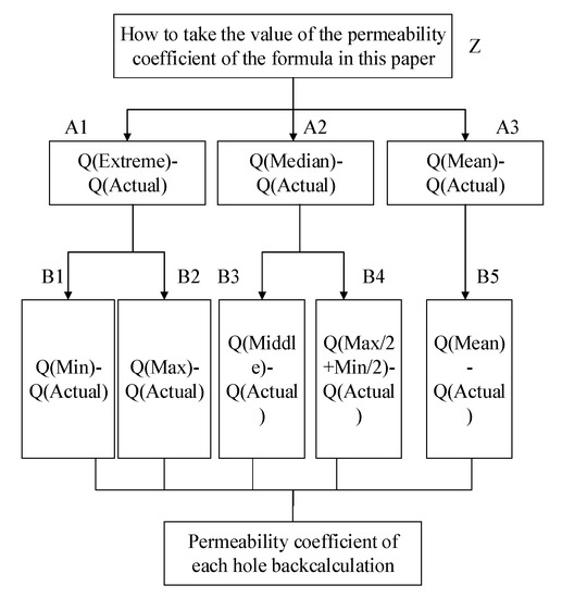
Figure 11.
Index system of AHP.
Table 7.
Judgment Matrix of Z to A.
Table 8.
Judgment Matrix of A1 to B.
Table 9.
Judgment Matrix of A2 to B.
We use to calculate and , i.e.,
Meanwhile, meets accuracy requirements at the same time.
4.2.2. Entropy Method Analysis
Entropy is generally used to measure the uncertainty of the data. The greater the amount of information, the smaller the data error, which also means smaller the entropy value, and vice versa. Therefore, the entropy value can be used to evaluate the dispersion of the data degree and determine the index weights.
- (1)
- Data standardization
There are 5 secondary indicators for each sample, and 15 sets of actual data from Qiyue Mountain were used, as shown in Table 10. Excavation without grouting listed in Table 11, Table 12, Table 13, Table 14, Table 15, Table 16 and Table 17.
Table 10.
Actual measurement data of different sections of Qiyue Mountain Tunnel.
Table 11.
Water inflow of ZD DK365+280 to +250 (0.3 MPA).
Table 12.
PDK365+327.5~+312.5 Circulation section (0.9 MPA).
Table 13.
ZD DK365+333 to +313 (1.7 MPA).
Table 14.
PDK365+335 to +308 circular segment (0.8 MPA).
Table 15.
ZDDK365+320 to +292.5 Circulation section (1.2 MPA).
Table 16.
ZDDK365+300 to +275 (1.2 MPA).
Table 17.
Water output from excavated sections of Gaoligong Mountain (S1ZK0).
Calculating the value of the infiltration coefficient by Equation (33), and then we can acquire the value of water inflow by Equation (32). Due to space, it is not described in detail. Take the value calculated by Equation (32) and the actual value of water inflow to constructs a 17 × 5 dimensional matrix and the matrix is normalized by using the smaller is better indicator .
- (2)
- Redundancy and Information Entropy calculation
Specific Gravity can be calculated with , while Information Entropy can be obtained by as shown below,
Meanwhile, redundancy is able to have as follow,
- (3)
- Calculation of weights
By using the formula of , we can have,
4.2.3. Combined Weighting Calculation
Whether subjective or objective, a one-sided description of the weights is one-sided and must be combined with both.
We assume,
where , and represents the importance of subjective and objective weights.
A linear weighting model was used, i.e., To make the degree of discrimination maximize, the linear model was constructed as follows,
We can set, , i.e.,
Taking the Lagrangian extremum theorem for calculation, the Lagrangian function is constructed as follows,
If , i.e.,
Substituting Equation (41) into Equation (40) and normalizing, we can obtain,
By calculating Equation (41), we can obtain the results in Table 18.
Table 18.
Parameter calculation results.
Substituting into Equation (40), the combined weight value is calculated as Table 19.
Table 19.
Weight values of different indexes.
In summary, if the dispersion of the permeability coefficients from the actual over-hole back-calculations at workface is not large, the recommended values for the permeability coefficients are: Mean > Median > Maximum > Minimum > Extreme mean.
4.3. Validation of Permeability Coefficient Weights for Formulae
We will verify the conclusion according to the following steps, show as Figure 12.
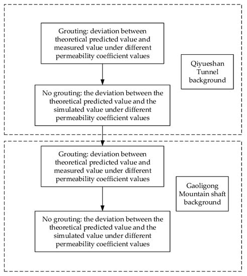
Figure 12.
Verification flow chart.
4.3.1. Comparative Analysis of Water Inflow at Different Sections of Qiyue Mountain Tunnel
- (1)
- Verification for slurry injection excavation water inflow
The excavated section is not continuous, so a point line approach is used for clarity of presentation. According to the calculations, it can be seen that the average and minimum values of the permeability coefficient can be calculated in a way that is very close to the measured influx of water.
However, we can know from Figure 13 that the very small value of the calculation of the water surge is generally less than the measured value, which is not enough safety reserve.
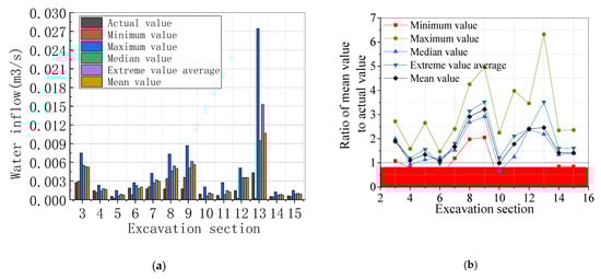
Figure 13.
Comparison of theoretical and measured values. (a) Comparison of theoretical and measured water inflow under different permeability coefficients; (b) Ratio of different theoretical water inflow to measured values. Where 3 stand for ZDDK365+333 to +313, 4 stand for ZDDK365+323 to +313, 5 stand for PDK365+313 to +308 (L), 6 stand for PDK365+316 to +308 (L), 7 stand for PDK365+319 to +308 (L), 8 stand for PDK365+322~+308 (L), 9 stand for PDK365+325 to +308 (L), 10 stand for YPDK365+315.5 to +312.5 (L), 11 stand for YPDK365+317.5 to +312.5 (L), 12 stand for ZDDK365+307.5 to +292.5 (L), 13 stand for ZDDK365+310.5 to +292.5 (L), 14 stand for ZDDK365+290 to +275, and 15 stand for ZDDK365+293 to +275.
Meanwhile, the water influx is calculated using a great value when the error is the largest, the size of the error is inversely proportional to the uniformity of the permeability coefficient taken. It is true that the use of very small values of the permeability coefficient can be a good way of reducing economic costs, but it is risky and should be used with caution.
- (2)
- Verification of water inflow at workface without slurry
As most of the site construction is slurry excavation for water-rich strata, there is a lack of actual measurement data without slurry excavation. However, with the research and application of simulation technology, this problem can be better dealt with. Here we use FLAC3D to simulate 15 sections of the Qiyue Mountain tunnel, taking the model size of 100 m × 40 m × 100 m, showing as Figure 14.
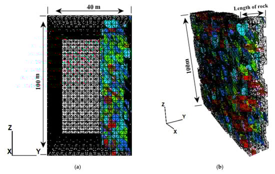
Figure 14.
Calculation model diagram. (a) Model size drawing, (b) Area of random distribution of permeability coefficients outside of grouting.
Considering the study focus on the seepage field, the model parameters were adopted from the site Class IV envelope parameters, see Table 20.
Table 20.
Site Class IV enclosure parameters of IV.
The permeability coefficient can be calculate with mean value, while the parameters for the different sections are shown in Table 21. For the permeability coefficients outside the range of overtopping in front of the workface, the values obtained from the n overtopping are considered to a log-normal distribution and expanded by one order of magnitude, which discretized as shown in Figure 15b with a permeability boundary.
Table 21.
Permeability coefficient after grouting in different sections.
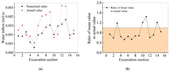
Figure 15.
Comparison of simulated and measured values for slurry excavation of shaft No. 1. (a) Comparison of simulated and measured values, (b) Ratio of simulated to measured values. Where 1 to 15 is same to above.
Meanwhile, the permeability coefficient obtained from the overtopping of the exploration horizon is equivalent to the overall permeability coefficient for that horizon. For the rock masses outside this range, the five sets of permeability coefficients B1, B2, B3, B4 and B5 obtained from the over-survey were randomly discretized using FLAC3D’s DFN plug-in.
Combined with the site conditions, the model through the control of permeability coefficient, grouting circle range and head height and other variables for different sections of the water influx calculation, and with the actual measurement, theoretical comparison are described in Figure 15.
As can be seen from Figure 15, the numerical simulation results are closer to the measured results, the deviation of the two is small, and the trend is similar. Therefore, it is considered that the numerical simulation method can effectively simulate the tunnel excavation water surge. The permeability coefficient distribution is similar to that of the grouting simulation, as show Figure 15. At the same time, different sections of the extraction model are compared with the theoretical values as follows.
Water influx for no grouting excavation of each hole permeability coefficient dispersion is large as displayed in Figure 16. If taking the extreme value of calculation, it will produce a great error, which is different with grouting. The use of intermediate values, extreme mean values, mean values of the calculated water influx values and simulated values are closer. The safety reserve is small when using intermediate values, while is too much when taking extreme mean. In summary, it is recommended that takes the mean value of each permeability coefficient to calculate and analyze the water influx when the dispersion of the permeability coefficient is not significant.
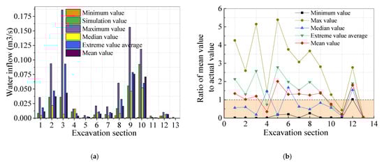
Figure 16.
Comparison of the measured values of the water inflow without grouting excavation. (a) Comparison of theoretical and measured water inflow under different permeability coefficients, (b) Ratio of different theoretical water inflow to measured values. Where 1 stand for ZDDK365+260 to +250, 2 stand for ZDDK365+270 to +250, 3 stand for ZDDK365+280 to +250, 4 stand for PDK365+317.5 to +312.5 circular segments, 5 stand for PDK365+322.5 to +312.5 circular segments, 6 stand for PDK365+327.5 to +312.5 circular segments, 7 stand for ZDDK365+302.5 to +292.5 circular segments, 8 stand for ZDDK365+311.5 to +292.5 circular segments, 9 stand for ZDDK365+315.5 to +292.5 circular segments, 10 stand for ZDDK365+321.5 to +292.5 circular segments, 11 stand for ZDDK365+284 to +275, 12 stand for ZDDK365+293 to +275, and 13 stand for ZDDK365+302.5 to +275.
4.3.2. Comparative Analysis of the Amount of Water Gushing from Different Sections of the Gaoligong Mountain Shaft
- (1)
- Verification of slurry injection excavation water inflow
The above selected values for the permeability coefficient of the tunnel excavation were verified. As for the shaft excavation, we use the main shaft of the Gaoligong Mountain No. 1 shaft to proof. Removing the discrete data on the amount of water gushing from the inspection holes, the amount of water gushing from the inspection holes in each working section are show in Table 17 and Table 22, while no grouting are shown in Table 23.
Table 22.
Water output from excavated sections of Gaoligong Mountain (S1ZK0).
Table 23.
Water output from different excavation sections (S1ZK0).
Combined with the data from Table 17, Table 22 and Table 23, Equation (32) is used to calculate the mean value of the permeability coefficient and the predicted value of the influx of water by using data from Equation (31). The predicted and measured values of water influx are compared in Figure 17.
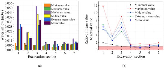
Figure 17.
No. 1 main well grouting excavation gushing water theoretical value and actual measured value comparison. (a) Comparison of theoretical and measured water inflow under different permeability coefficients, (b) Ratio of different theoretical water surges to measured values. Where 1 stand for S1ZK0+198.7 to +278.7, 2 stand for S1ZK0+425.5 to +505.5, 3 stand for S1ZK0 +497.5 to +597.5, 4 stand for S1ZK0+580.3 to +640.3, 5 stand for S1ZK0+619.9 to +679.9, 6 stand for S1ZK0 +652.3 to +712.3, 7 stand for S1ZK0+691.9 to +751.9.
We can conclude that the excavation Sections 1 and 3–7 at the theoretical value of the water surge and the measured value is closer from Figure 17. Theoretical values and measured values have a large error at the excavation Sections 1 and 3, which is because engineering needs to supplement the slurry uninterrupted to make sure the safe of excavation when meeting great water inflow. Minimum and Median values do not have sufficient safety reserves, and the economic cost of the maximum value is too high. We find that using the average value of water inflow is closer to the actual, and make sure a certain amount of safety reserves.
- (2)
- Verification of water inflow at the workface of excavation without slurry
We use numerical methods to predict the actual of excavation water inflow without slurry. Take the model size of 160 m × 160 m × 130 m, and for the length of the probe hole range to take the equivalent permeability coefficient. Meanwhile, as for the probe hollow range, we use five groups of permeability coefficient values for random discrete as shown in Figure 18b. The data obtained from the overtopping of the water probe holes are shown in Table 23. The use of Equation (32) to calculate the value of the water inflow and simulation values compared in Figure 19.
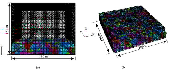
Figure 18.
Calculation model diagram of the shaft. (a) Shaft 1 main shaft permeability coefficient equivalent with stochastic area, (b) Area of random distribution of permeability coefficients.
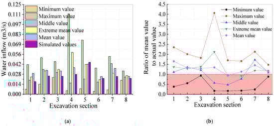
Figure 19.
Comparison of simulated and measured values for the main shaft of Shaft No. 1 without grouting excavation. (a) Comparison of theoretical and measured water inflow under different permeability coefficients, (b) Ratio of different theoretical water surges to measured values. Where 1 stand for S1ZK0+198.7 to +278.7, 2 stand for S1ZK0+263.5 to +315.5, 3 stand for S1ZK0+263.5 to +323.5,4 stand for S1ZK0+263.5 to +333.5, 5 stand for S1ZK0+295.9 to +375.9, 6 stand for S1ZK0+364.3 to +444.3, 7 stand for S1ZK0+497.5 to +597.5, 8 stand for S1ZK0+730.9 to +778.484.
As can be seen from Figure 19, the use of extreme values for the calculations produces large errors. At smaller and uniform permeability coefficients, the simulated values are closer to the theoretical values. At the same time, the use of extreme values for the calculations produces large errors as shown in Figure 19. The more uniform the value of the permeability coefficient is, the closer it is to the simulated value. The theoretical value obtained by using the mean value of the extreme value of the permeability coefficient and the mean value is closer to the simulated value. However, the mean value is a better relative fit.
This section validates the results of the weight value calculations in the previous section in relation to the tunnel and shaft works and draws the following conclusions:
The results show that the minimum value is always lower than the measured value. In addition, only the mean value can float around the measured value stably. Considering the safety reserves and economic costs, in the case of permeability coefficient dispersion is not large, the permeability coefficients mean value is reasonable for the analysis of water influx.
4.4. Verification of the Feasibility of Excavation Standards
The actual measured data of the water inflow in the main shaft and sub-shaft of Goligong Mountains No. 1 shaft are used to proof the method. Gaoligong Mountains No. 1 shaft main shaft S1ZK0+130.5 to +230.5, sub shaft S1FK0+290.5 to +370.5, sub shaft S1FK0+358.9 to +438.9, sub shaft S1FK0+427.3 to +507.3 are not grouted, and the water output from the exploratory boreholes in these excavated sections after over-exploration is shown in Table 24.
Table 24.
Water output from different excavation sections.
According to the Chinese standard, Goligong Mountains considers that water operation with water is allowed when the water volume in the water exploration hole is less than 0.0028 m3/s. The permeability coefficients for each hole calculated using Equation (32) are shown in Table 25. The excavation is reserved for a slurry thickness of 10 m, and the calculated influx is compared with the actual excavation in Table 26. The actual and predicted water inflow are relatively close and are less than the drainage capacity of the project.
Table 25.
Values of permeability coefficients for different excavation sections.
Table 26.
Different excavation sections with predicted and measured water inflow.
In addition, the data before and after grouting are shown in Table 27 for Qiyue Mountain of grouting end criteria. We can see that the predicted water inflow from the excavation without grouting is much greater than the project drainage capacity and requires grouting. At the end of grouting, the corresponding grouting excavation surge is calculated to be less than the drainage capacity of the project. Therefore, excavation is allowed. Water inflow of the sections are not much different from the actual measured value, it is believed that this system has a certain degree of excavation standard judgment ability.
Table 27.
Different excavation sections before and after the slurry injection of water influx and measured value comparison.
5. Conclusions
- (1)
- There is a large difference between the confined aquifer in steeply dipping large, fractured rock and the ideal confined aquifer. Therefore, the equivalent continuous medium cannot be used to simulate this type of rock mass. The numerical simulation method proposed in this paper based on the dual pore medium model effectively explains the cause of high water pressure in the Gaoligong Mountains, i.e., the fractures penetrate the confined aquifer leads to the total hydraulic head is equal between fractures and aquifers.
- (2)
- In the Gaoligong Mountain project application, this paper proposes the prediction formula of slurry water inflow is closer to the measured value and simulated value of grouting compared to the original pressurized to unpressurized formula, and has sufficient safety reserves. Furthermore, the prediction formula for water inflow without grouting is similar to the simulated value without grouting. The smaller the permeability coefficient, the smaller the prediction error.
- (3)
- It is recommended that taking the mean value to calculate the water inflow when the dispersion of the permeability coefficients of each hole is not too large, while the minimum value is not recommended for calculation. The grouting evaluation system proposed in this paper has a certain degree of feasibility and reference value, verified by actual engineering.
Author Contributions
Conceptualization, J.L. and Y.W.; methodology, J.L.; software, J.L.; validation, J.L., C.W. and Q.H.; formal analysis, J.L.; investigation, J.L.; resources, J.L.; data curation, J.L.; writing—original draft preparation, J.L.; writing—review and editing, J.L.; visualization, J.L.; supervision, Y.W.; project administration, J.L.; funding acquisition, Y.W. All authors have read and agreed to the published version of the manuscript.
Funding
The authors acknowledge the financial support provided by the National Natural Science Foundation of China Projects funding (51478037).
Institutional Review Board Statement
Not applicable.
Informed Consent Statement
Not applicable.
Data Availability Statement
Not applicable.
Conflicts of Interest
The authors declare no conflict of interest.
Nomenclature
| Spherical coordinate radius | |
| Total head | |
| Total head outside the ball | |
| Total head inside the ball | |
| Formula parameters | |
| Water inflow | |
| Angle between the radius of the sphere and the axis of the shaft | |
| Permeability coefficient of Grouting ring | |
| Permeability coefficient of rock | |
| Aquifer thickness | |
| Shaft radius |
References
- Polubarinova-Kochina, P.Y. Theory of Ground Water Movement; Princeton University Press: Princeton, NJ, USA, 1962. [Google Scholar]
- Goodman, R.E.; Moye, D.G.; van Schalkwyk, A. Ground water inflows during tunnel driving. Eng. Geol. 1965, 1, 39–56. [Google Scholar]
- Freeze, R.A.; Cherry, J.A. Groundwater; Prentice-Hall Inc.: Englewood, NJ, USA, 1979. [Google Scholar]
- Tal, A.; Dagan, G. Flow toward storage tunnels beneath a water Table: 1. Two-dimensional-flow. Water Resour. Res. 1983, 1, 241–250. [Google Scholar] [CrossRef]
- Tal, A.; Dagan, G. Flow toward storage tunnels beneath a watertable three dimensional flow. Water Resour. Res. 1984, 9, 1216–1224. [Google Scholar] [CrossRef]
- Strack, O.D.L. Groundwater Mechanics; Prentice-Hall Inc.: Englewood, NJ, USA, 1989. [Google Scholar]
- Anagnostou, G. The influence of tunnel excavation on the hydraulic head. Int. J. Numer. Anal. Methods Geomech. 1995, 10, 725–746. [Google Scholar] [CrossRef]
- Chisyaki, T. A study on confined flow of ground water through a tunnel. Ground Water 1984, 2, 162–167. [Google Scholar] [CrossRef]
- Meiri, D. Unconfined groundwate flow calculation into tunnel. J. Hydrol. 1982, 1, 69–75. [Google Scholar]
- Domenico, P.A.; Schwartz, F.W. Physical and Chemical Hydrogeology; John Wiley and Sons: New York, NY, USA, 1990. [Google Scholar]
- Lei, S. An analytical solution for steady flow into a tunnel. Ground Water 1999, 37, 23–26. [Google Scholar] [CrossRef]
- Park, K.H.; Owatsiriwong, A.; Lee, J.G. Analytical solution for steady-state groundwater inflow into a drained circular tunnel in a semi-infinite aquifer: A revisit. Tunn. Undergr. Space Technol. 2008, 22, 206–209. [Google Scholar] [CrossRef]
- El Tani, M. Circular tunnel in a semi-infinite aquifer. Tunn. Undergr. Space Technol. 2003, 18, 49–55. [Google Scholar] [CrossRef]
- Kolymbas, D.; Wagner, P. Groundwater ingress to tunnels—The exact analytical solution. Tunn. Undergr. Space Technol. 2007, 22, 23–27. [Google Scholar] [CrossRef]
- Luo, H.; Chuan, Q. Tritium in groundwater in Japan. Water Wastewater 1972, 3, 69–72. [Google Scholar]
- Luo, H. Application of natural tritium in groundwater exploration. Water Wastewater 1968, 1, 33–34. [Google Scholar]
- Zuo, T. Approximate analysis of unsteady ground water excavated in rock cavern. Tunnels Undergr. 1983, 11, 30–36. [Google Scholar]
- Zhu, D.; Li, Q. Method for predicting tunnel water inflow. Eng. Investig. 2000, 1, 18–22. [Google Scholar]
- Wang, X.; Wang, M.; Zhang, M. Study on external water pressure of water blocking and drainage limiting lining of mountain tunnel. J. Geotech. Eng. 2005, 27, 124–127. [Google Scholar]
- Ding, W.; Li, S.; Xu, B. Application of analytical formula of tunnel water inflow in Subsea Tunnel Engineering. J. Undergr. Space Eng. 2008, 1, 662–664. [Google Scholar]
- Wang, J. Further discussion on water pressure of tunnel lining. Mod. Tunn. Technol. 2003, 3, 5–9. [Google Scholar]
- Hu, P.; Tan, Z.; Wang, M. Analytical solution of seepage flow in underground subsea tunnel and its application. Chin. Eng. Sci. 2009, 11, 66–70. [Google Scholar]
- Fu, H.; Li, Z.; Cheng, G. Prediction of tunnel water inflow in fault affected area based on conformal mapping. J. Huazhong Univ. Sci. Technol. 2021, 49, 86–92. [Google Scholar]
- Li, Q.; Ito, K.; Wu, Z.; Lowry, C.S.; Loheide, S.P., II. COMSOL multiphysics: A novel approach to ground water modeling. Ground Water 2009, 47, 480–487. [Google Scholar] [CrossRef]
- Zhao, C.; Wang, H.; Wang, S. Construction of drainage numerical model and water inflow analysis of inclined group holes in coal mine. J. Min. Saf. Eng. 2021, 38, 687–694. [Google Scholar]
- Li, J.H.; Zhang, Z.X. Quick Start Guide of FLAC3D; China Building Industry Press: Beijing, China, 2016; pp. 1–14. [Google Scholar]
- Chen, Y.M.; Xu, L.M. Basics of FLAC/FLAC3D and Engineering Example; China Water Power Press: Beijing, China, 2013; pp. 1–5. [Google Scholar]
- Tian, G.; Wang, J. Prediction and analysis of water inflow in hanglaiwan mine based on numerical simulation. Energy Technol. Manag. 2021, 46, 13–16. [Google Scholar]
- Zhou, W. Study on water inflow prediction technology of Guanshan tunnel on Tianping line. Mod. Tunn. Technol. 2021, 58, 22–30. [Google Scholar]
- Gong, H.; Liu, S.; Li, Z. Research on numerical simulation and prediction of mine water inflow based on Visual Modflow. Coal Technol. 2018, 37, 155–157. [Google Scholar]
- Bi, Z. Study on Numerical Simulation of mine water inflow in Daping Coal Mine. Liaoning Univ. Eng. Technol. 2010, 23, 23–30. [Google Scholar]
- Zhang, W.; Dong, S. Water inrush prediction of karst water filled deposit and its impact on surrounding water sources—A case study of a coal mine in Ordos. North. Environ. 2012, 27, 29–32. [Google Scholar]
- Hwang, J.-H.; Lu, C.-C. A semi-analytical method for analyzing the tunnel water inflow. Tunn. Undergr. Space Technol. 2007, 22, 39–46. [Google Scholar] [CrossRef]
- Dayangshimaji. Railway Technology Research Report; University of Tokyo Press: Tokyo, Japan, 1983. [Google Scholar]
Publisher’s Note: MDPI stays neutral with regard to jurisdictional claims in published maps and institutional affiliations. |
© 2021 by the authors. Licensee MDPI, Basel, Switzerland. This article is an open access article distributed under the terms and conditions of the Creative Commons Attribution (CC BY) license (https://creativecommons.org/licenses/by/4.0/).