Fluid-Structure Interaction Analysis of Aircraft Hydraulic Pipe with Complex Constraints Based on Discrete Time Transfer Matrix Method

Abstract

Fluid-structure interaction (FSI) is prevalent in aircraft hydraulic pipes due to high-pressure fluid pulsation, complex pipe path routing and boundary constraints, which pose a serious threat to the safety and reliability of the aircraft hydraulic system. This paper focuses on the FSI response of aircraft hydraulic pipes with complex constraints. A comprehensive fourteen-equation model for describing the FSI of pipe conveying fluid with wide pressure and Reynolds number range is proposed. The excitation models and complex boundary constraints of liquid-filled pipes are established. Moreover, based on the transfer matrix method (TMM), combined with the time discreteness and analytical integral method, a discrete time transfer matrix method (DTTMM) for solving the FSI fourteen-equation model in time domain is presented. Then, the numerical solution and experiment of an ARJ21-700 aircraft hydraulic pipe with complex constraints is carried out with four working conditions. The obtained results verify the correctness of the proposed model and solution method, and reveal the universal laws of the FSI response about aircraft hydraulic pipes, which can also provide theoretical and experimental references for modeling, solutions and verification in the FSI analysis of pipe conveying fluid.

1. Introduction

Hydraulic systems are widely employed in aerospace and other significant industry departments by their high power density and high immunity to load variations. The fluid-structure interaction (FSI) of hydraulic pipes can be induced by sudden starting or stopping of the hydraulic pump, fast opening or closing valve, pulsation of fluid in the pipe and external mechanical excitation. The FSI in aircraft hydraulic pipeline systems, due to complex flow patterns, a wide range of pressure, complex pipe path routing and boundary constraints, can cause pipeline system vibration failures [1], which directly affect the work reliability of the whole pipeline system and the flight safety of the aircraft. The vibration characteristics of aircraft pipelines are gradually becoming more concerning over recent years [2,3,4,5,6,7,8,9,10]. Therefore, for the FSI analysis of aircraft hydraulic pipes, it is of great theoretical and practical significance to establish a comprehensive model to provide accurate solution methods and experimental verifications.

In recent decades, the investigations for the FSI characteristics of pipe conveying fluids have been reported extensively, including analytical models, numerical calculations and tests. So far, the various FSI models of the pipe conveying fluid used by scholars from various countries are basically developed from the water hammer theory presented by Joukowsky [11]. The following representative research works are summarized: Skalak [12] presented the classical four-equation model, where the water hammer model was extended and combined with the axial stress model of the pipe and the friction coupling and damping effect were ignored. Then, the four-equation model was extended by Wiggert et al. [13] and You et al. [14], where Poisson coupling was taken into account. Based on the work of Skalak, Walker and Phillips [15] presented the six-equation model containing the radial deformation of the pipe and the added mass of the fluid. An eight-equation model considering axial movement of the free end of the pipe for the vibration analysis of the two-dimensional pipe had been built by Davidson [16]. Based on the fluid wave equation and Timoshenko beam model, a fourteen-equation model was firstly proposed by Wiggert [17], where the pulsation of fluid, the axial deformation, transverse shear deformation, bending deformation of the pipe and the torsional deflection of the pipe wall were considered. After that, considering the friction coupling, Bourbon and junction coupling, the fourteen-equation model was extended and followed by a majority of researchers [9,10,18,19]. The establishment of a more applicable and comprehensive FSI model awaits further study.

Solution methods and experimental validations of FSI in the fluid-filled pipe mainly focused on the time domain and frequency domain. The time domain methods are usually used for the transient response analysis of the fluid and pipe, and in the frequency domain the free vibration and forced vibration response are paid much attention [17]. This paper places emphasis on time domain methods and verification; the literature of the main frequency domain solution methods is summarized briefly: the Transfer Matrix Method (TMM) [9,10,18,19,20,21], Component Synthesis Method (CSM) [22], wave propagation method [23] and Laplace transform method [9,10,18]. The common methods of the time domain solution include: the Method of Characteristics (MOC), Transfer Matrix Method (TMM) [24,25,26], Finite Element Method (FEM) [27,28,29] and MOC-FEM [30,31]. As an approximate method for solving hyperbolic partial differential equations, the MOC has become the most commonly used method in the time domain. TMM is a classical method of analyzing the system dynamics, simple solution process and high accuracy; these are the main advantages of this method. The representative research works are summarized: Wiggert et al. [13,32] used the MOC to simulate a fluid-filled copper pipe under pulse excitation, and verified experiments were carried out. The concrete steps and common simple boundary conditions for solving the fourteen-equation model through MOC were discussed in detail by Tijsseling [33]. Ouyang et al. [34] used the MOC to analyze the fluctuating pressure of the two-dimensional aircraft hydraulic pipe. In practical usage, the time step and the length of the pipe segments must conform to the characteristic equation, which causes some limitations in the scope of application, calculation efficiency and calculation accuracy of the MOC. Other time domain solution methods based on the TMM were developed and received satisfactory results. Based on the TMM, Tentarelli [35] presented an appropriate set of dynamic equations and analytical methods, which is applicable to simple segments and complex tubing systems. Based on the TMM for solving the eight-equation model, Gale and Tiselj [36] studied the time domain response of the pressure wave and pipe wall vibration of the single elbow. It is an important research topic to establish a universal and efficient time domain solution in the field of the solution of FSI in the fluid-filled pipe.

From the reviewed works, most of the current strategies are excellent in handling the common simple pipe conveying fluid FSI problems available. However, the FSI theoretical models used in the existing research works are simplified and not comprehensive enough; there are some limitations in the scope of application, calculation efficiency and calculation accuracy of the earlier time domain solution methods; moreover, the pipe structure and boundary conditions used in the past research are relatively simple, and the studies which can be used to guide engineering practice are less investigated.

In this paper, a comprehensive FSI model of liquid-filled pipe, including the friction coupling, the gravity, centrifugal force, Coriolis force and the moment of inertia caused by fluid within pipe, is proposed. Various excitation models and complex boundary constraints are established. A time domain solution method for solving the FSI fourteen-equation model by the discrete time transfer matrix method (DTTMM) is presented. The numerical solution and experiment of an ARJ21-700 aircraft hydraulic pipe with complex constraints is carried out with four working conditions to verify the proposed model and solution method. Some universal laws of FSI response about aircraft hydraulic pipe are revealed, and the little result errors are calculated and analyzed.

2. Theoretical Modeling

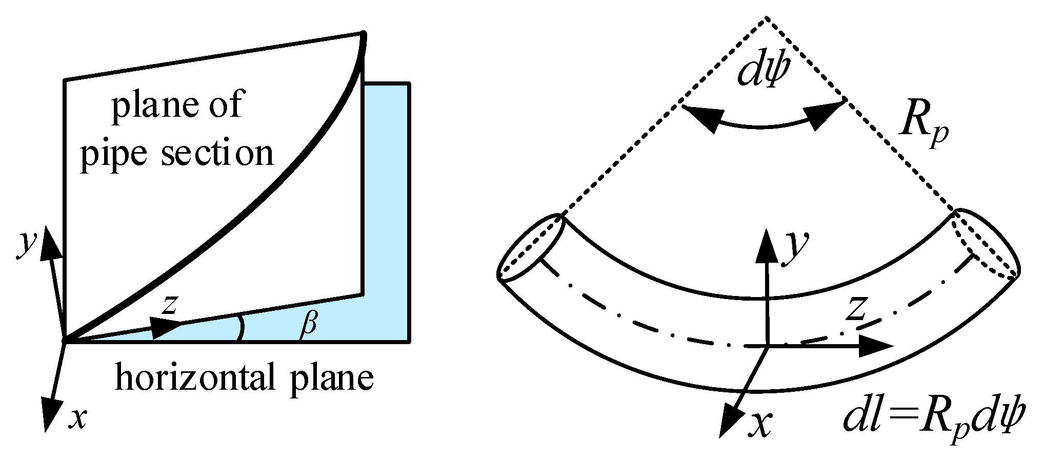
2.1. FSI Fourteen-Equation Model

There are seven degrees of freedom when the fluid-filled pipe vibrates in the approximate form of the beam modal, and each of these degrees of freedom can be expressed by the corresponding velocity (angular velocity) and force (torque). Therefore, the movement state of fluid-filled pipe can be completely described by the FSI fourteen-equation model. In this section, a more comprehensive fourteen equations for a pipe section (see Figure 1) are derived based on [9,18]. The basic assumptions for the presented model include: a long wavelength relative to pipe diameter, low Mach numbers; absence of liquid column separation or air bubbles, linear elastic behavior of piping material and fluid, and negligible inertia in the radial direction. Axial motion equations include the modified friction coupling model, and the impacts of gravity, centrifugal force, Coriolis force and the moment of inertia caused by fluid within pipe are taken into account. The nomenclature of parameters in the FSI fourteen-equation model is listed in

Table A1. Nomenclature of parameters in theoretical modeling.

Parameter	Definition	Unit	Parameter	Definition	Unit
R	Inner radius of pipe	m	l	Length of pipe	m
R0	Outer radius of pipe	m	$\theta$	Deflection angle of pipe	rad
D	Pipe diameter	m	ρ	Density	kg/m3
A	Cross-sectional area	m2	rp	Centrifugal radius of fluid	m
M	Moment	Nm	$\beta$	Angle between pipe and Horizontal plane	rad
G	Shear modulus	Pa	$\dot{\theta }$	Angular velocity of pipe wall	rad/s
V	Fluid velocity	m/s	$\dot{\omega }$	Pipe velocity	m/s
P	Fluid pressure	MPa	$\psi$	Bending angle of pipe	rad
K	Fluid bulk modulus	MPa	f	Forces in cross-section	N
$K^{\prime }$	Corrected fluid bulk modulus	MPa	$\tau$	Shear stress of pipe wall	Pa
I	Flexure moment of inertia	m4	σ	Stress	N/m2
J	Polar moment of inertia	m4	k	Shear coefficient	-
T	External moment of constraints	m4	$v$	Poisson’s ratio	-
e	Thickness of pipe wall	m	$\epsilon$	Strain	-
m	Mass	g	x,y,z	Directional subscripts	-
E	Modulus of elasticity	MPa	f,p	Structural subscripts	-

(Appendix A).

1. Four equations of axial motion.

$$\frac{\partial V_f}{\partial t}+V\frac{\partial V_f}{\partial l}+\frac{1}{{\rho }_f}\frac{\partial P}{\partial l}+\frac{4}{{\rho }_{f}D}{\tau }_w+g\sin \beta =0$$

(1)

$$\frac{\partial {\dot{w}}_z}{\partial t}+\frac{1}{{\rho }_p{A}_p}\frac{\partial f_z}{\partial l}+\frac{1}{{\rho }_p{A}_p}\frac{f_y}{R_p}-\frac{4}{{\rho }_p{A}_p{\rho }_{f}D}{\tau }_w+g\sin \beta -\frac{f_{ez}}{{\rho }_p{A}_p}=0$$

(2)

$$\frac{\partial P}{\partial t}-2v{K}^{\prime }\frac{\partial {\dot{w}}_z}{\partial l}+K^{\prime }\frac{\partial V_f}{\partial l}+K^{\prime }(1-2v)\frac{{\dot{w}}_y}{R_w}=0$$

(3)

$$\frac{\partial f_z}{\partial t}+\left[E{A}_p+\frac{4v^2{K}^{\prime }{A}_p}{e_R\left(2+e_R\right)}\right]\frac{\partial {\dot{w}}_z}{\partial l}-\frac{2v{K}^{\prime }{A}_p}{e_R\left(2+e_R\right)}\frac{\partial V_f}{\partial l}+\left[E{A}_p+\frac{2v(1-2v)K^{\prime }{A}_p}{e_R\left(2+e_R\right)}\right]\frac{{\dot{w}}_y}{R_p}=0$$

(4)

2. Four equations of x-z planar motion.

$$\frac{\partial M_y}{\partial t}+E{I}_p\frac{\partial {\dot{\theta }}_y}{\partial l}-E{I}_p\frac{{\dot{\theta }}_z}{R_p}=0$$

(5)

$$\frac{\partial {\dot{w}}_x}{\partial t}+\frac{1}{m}\frac{\partial f_x}{\partial l}-\frac{2m_{f}V}{m}\frac{\partial {\dot{w}}_x}{\partial l}-\frac{m_f{V}^2+P{A}_f}{m}\left(\frac{1}{E{I}_p}{M}_y-\frac{{\theta }_z}{R_p}\right)+g\cos \beta -\frac{1}{m}{f}_{ex}=0$$

(6)

$$\frac{\partial f_x}{\partial t}+\kappa G{A}_p\frac{\partial {\dot{w}}_x}{\partial l}-\kappa G{A}_p{\dot{\theta }}_y=0$$

(7)

$$\frac{\partial {\dot{\theta }}_y}{\partial t}+\frac{1}{T_y}\frac{\partial M_y}{\partial l}+\frac{1}{T_y}{f}_x-\frac{1}{T_y{R}_p}{M}_z-\frac{1}{T_y}{M}_{ey}=0$$

(8)

3. Four equations of y-z planar motion.

$$\frac{\partial M_x}{\partial t}+E{I}_p\frac{\partial {\dot{\theta }}_x}{\partial l}=0$$

(9)

$$\frac{\partial {\dot{w}}_y}{\partial t}+\frac{1}{m}\frac{\partial f_y}{\partial l}+\frac{2m_{f}V}{m}\frac{\partial {\dot{w}}_y}{\partial l}+\frac{m_f{V}^2+P{A}_f}{m}\left(\frac{M_x}{E{I}_p}-\frac{1}{R_p}\right)-\frac{1}{m{R}_p}{f}_z+g\cos \beta -\frac{1}{m}{f}_{ey}=0$$

(10)

$$\frac{\partial f_y}{\partial t}+\kappa G{A}_p\frac{\partial {\dot{w}}_y}{\partial l}+\kappa G{A}_p{\dot{\theta }}_x-\frac{\kappa G{A}_p}{R_p}{\dot{w}}_z=0$$

(11)

$$\frac{\partial {\dot{\theta }}_x}{\partial t}+\frac{1}{T_x}\frac{\partial M_x}{\partial l}-\frac{1}{T_x}{f}_y-\frac{1}{T_x}{M}_{ey}=0$$

(12)

4. Two equations of torsion motion.

$$\frac{\partial M_z}{\partial t}+G{J}_p\frac{\partial {\dot{\theta }}_z}{\partial l}+\frac{G{J}_p}{R_p}{\dot{\theta }}_y=0$$

(13)

$$\frac{\partial {\dot{\theta }}_z}{\partial t}+\frac{1}{{\rho }_p{J}_p}\frac{\partial M_z}{\partial l}+\frac{1}{{\rho }_p{J}_p{R}_p}{M}_y-\frac{1}{{\rho }_p{J}_p}{M}_{ez}=0$$

(14)

where

$${\tau }_w={\tau }_{ws}+{\tau }_{wuz}+{\tau }_{wub}=\frac{\rho fV\left|V\right|}{8}+k\frac{4\rho V}{D}{\displaystyle {\int }_0^t\frac{\partial V\left(t\right)}{\partial t}\frac{C_1{e}^{-C_{2}t}}{\sqrt{\pi t}}dt}+(1-k)\frac{\rho D}{4}·k_3\left(\frac{\partial V}{\partial t}-\alpha \frac{\partial V}{\partial z}\right)$$

(15)

$$C_1=\frac{R}{2\sqrt{v_w}},C_2=\frac{0.135v_w}{R^2}R{e}^{k_4}$$

(16)

$$k_3=\sqrt{\frac{7.41/R{e}^{k_4}}{2}},k_4=\lg (14.3/R{e}^{0.05})$$

(17)

$$\alpha =\frac{\sqrt{K/{\rho }_f}}{\sqrt{1+DK/eE}}$$

(18)

Equation (15), ${\tau }_{ws}$ is the wall shear friction in steady flow, ${\tau }_{wuz}$ is the Zielke additional shear friction term in unsteady flow and ${\tau }_{wub}$ is the Brunone additional shear friction term in unsteady flow. For the FSI analysis of pipe conveying fluid within a wide range of the Reynolds number, the selection coefficient k needs to be defined. When the fluid inside the pipe is in the transient laminar flow and the low-Reynolds-number turbulence (Reynolds number is less than 2320), k = 1, instead, when the fluid under the unsteady turbulence state and high-Reynolds-number turbulence (Reynolds number is greater than 2320), k = 0.

2.2. Excitation Matrix Model

Excitation matrix, as a necessary condition for solving the FSI model through the aforementioned method, with the basic idea of excitation matrix reviewed in [21], mainly includes fluid excitation (closed end, pressure boundary, velocity boundary and flow pulsation) and solid excitation (mechanical shock and simple harmonic vibration). In this subsection, a general excitation matrix model and the flow pulsation excitation model of axial piston pump are proposed, which are suitable for solving the FSI fourteen-equation model by the discrete time transfer matrix method (DTTMM).

The excitation vectors at both ends of the pipe are as follows:

$$\{\begin{array}{l}{\left[{\mathbf{Q}}_0\right]}_{7\times 1}={\left[\begin{array}{ccccccc}V(0,t_k)& f_{ez}(0,t_{k-1})& f_{ex}(0,t_{k-1})& M_{ey}(0,t_{k-1})& f_{ey}(0,t_{k-1})& M_{ex}(0,t_{k-1})& M_{ez}(0,t_{k-1})\end{array}\right]}^{\mathrm{T}}\\ {\left[{\mathbf{Q}}_L\right]}_{7\times 1}={\left[\begin{array}{ccccccc}V(L,t_k)& f_{ez}(L,t_{k-1})& f_{ex}(L,t_{k-1})& M_{ey}(L,t_{k-1})& f_{ey}(L,t_{k-1})& M_{ex}(L,t_{k-1})& M_{ez}(L,t_{k-1})\end{array}\right]}^{\mathrm{T}}\end{array}$$

(19)

As an important characteristic of axial piston pump and a key excitation form, the flow pulsation model has been investigated in previous works [9,37,38]. The theoretical formula of piston pump flow is shown as the following:

$$q_t=2AznR\tan \gamma =\frac{\pi d^2}{2}znR\tan \gamma$$

(20)

where A is the cross-section of the piston, z is the number of pistons, n is the speed of cylinder block, $\gamma$ is the tilt angle of swash plate, and R is the diameter of the piston.

The instantaneous flow of piston pump could be expressed as:

$$q_{sh}={\displaystyle \sum _{i=1}^{{\mathrm{z}}_0}A}{v}_i=AR\omega \tan \gamma {\displaystyle \sum _{i=1}^{z_0}\sin }{\phi }_i$$

(21)

where z₀ is the number of pistons in the oil drain chamber, v_i is the axial velocity of piston located in the oil drain chamber and ${\phi }_i$ is the relative rotation angle of piston located in the oil drain chamber.

The flow pulsation excitation could be represented by flow velocity, and the detailed calculation process is: the first n-order spectrum and its function expressions can be obtained by FFT transformation of the time-domain flow pulsation, then, add the function expressions corresponding to the first n-order harmonics together to obtain V.

$$V_e=V_0+V_{A1}\sin {\omega }_{1}t+V_{A2}\sin {\omega }_{2}t+V_{A3}\sin {\omega }_{3}t+V_{A4}\sin {\omega }_{4}t$$

(22)

2.3. Boundary Matrix Model

A vital step for getting a solution of the FSI model is to establish the relationship of the vector between the pipe and the external constraints. The matrix models of common constraints, such as fixed constraints, elastic constraints and free constraints, were discussed in [16,20,35,39]. With this research, complex boundary constraints involving added mass and stiffness are studied in this subsection.

As for a single pipe section microelement or a node of pipe, there will be force balance and motion continuity, relationships which are always forces or angular moments sum to zero, and linear or angular velocity, which are equal. Thus, the balance equation of force and moment of the single pipe section microelement or a node of pipe can be written as:

$$\{\begin{array}{l}{f}_o(0,t_i)+k(\omega (0,t_{i-1})+\dot{\omega }(0,t_i)\Delta t)=f_e(0,t_i)-f(0,t_i)\\ M_o(0,t_i)+t(\theta (0,t_{i-1})+\dot{\theta }(0,t_i)\Delta t)=M_e(0,t_i)-M(0,t_i)\end{array}$$

(23)

Then, as an example, the boundary matrices of closed ends and complex constraints include elasticity; added mass and inertia are given (Appendix B).

2.4. Middle Constraint Matrix Model

Middle constraint is the indispensable configuration in the pipe system; the modeling method and application of the simple middle constraint were investigated in [40,41,42,43]. The middle constraint matrix, including the concentrated mass and additional stiffness, is presented by using the point transfer matrix in this subsection.

Based on the force balance and motion continuity, the relation between state vectors at either end of the middle constraint node could be expressed as:

$${\mathsf{\phi }}_{i+1}(0,t_i)={\mathbf{N}}_i(t_i){\mathsf{\phi }}_i(L_i,t_i)$$

(24)

${\mathbf{N}}_i$ is the constraint matrix of the middle constraint, which represents the transitive relation at the discontinuity of the series connection pipe. If there are no constraints at the connection location and the diameter and material of the pipe are unchanged, ${\mathbf{N}}_i$ is unit matrix.

$${\mathbf{N}}_i=\left[\begin{array}{cccccccccccccc}1& 0& 0& 0& 0& 0& 0& 0& 0& 0& 0& 0& 0& 0\\ 0& 1& 0& 0& 0& 0& 0& 0& 0& 0& 0& 0& 0& 0\\ 0& 0& 1& 0& 0& 0& 0& 0& 0& 0& 0& 0& 0& 0\\ 0& 0& K_{zi}& 1& 0& 0& 0& 0& 0& 0& 0& 0& 0& 0\\ 0& 0& 0& 0& 1& 0& 0& 0& 0& 0& 0& 0& 0& 0\\ 0& 0& 0& 0& 0& 1& 0& 0& 0& 0& 0& 0& 0& 0\\ 0& 0& 0& 0& 0& T_{yi}& 1& 0& 0& 0& 0& 0& 0& 0\\ 0& 0& 0& 0& 0& 0& K_{xi}& 1& 0& 0& 0& 0& 0& 0\\ 0& 0& 0& 0& 0& 0& 0& 0& 1& 0& 0& 0& 0& 0\\ 0& 0& 0& 0& 0& 0& 0& 0& 0& 1& 0& 0& 0& 0\\ 0& 0& 0& 0& 0& 0& 0& 0& 0& T_{xi}& 1& 0& 0& 0\\ 0& 0& 0& 0& 0& 0& 0& 0& 0& 0& K_{yi}& 1& 0& 0\\ 0& 0& 0& 0& 0& 0& 0& 0& 0& 0& 0& 0& 1& 0\\ 0& 0& 0& 0& 0& 0& 0& 0& 0& 0& 0& 0& T_{zi}& 1\end{array}\right]$$

(25)

where $K_{(i)}$ and $T_{(i)}$ are translational stiffness and rotational stiffness, respectively.

The field transfer matrix (see Equation (41)) of the pipe can be expressed as:

$${\mathbf{U}}_{\mathrm{all}}(t_i)={\mathbf{U}}_N(L_N,t_i)\cdots {\mathbf{U}}_{i+1}(L_{i+1},t_i){\mathbf{N}}_i(t_i){\mathbf{U}}_i(L_i,t_i)\cdots {\mathbf{U}}_1(L_1,t_i)$$

(26)

The application methods of ${\mathbf{N}}_i$ and ${\mathbf{U}}_{\mathrm{all}}(t_i)$ in solving the FSI fourteen-equation model are specified in the next section.

3. Discrete Time Transfer Matrix Method

Referencing the deduction process in [9,18,44], the time domain solution (DTTMM) of the FSI fourteen-equation model is studied in this section. The fourteen equations in Section 2.1 can be expressed with matrixes as:

$$\mathbf{A}\frac{\partial \mathsf{\Phi }(z,t)}{\partial t}+\mathbf{B}\frac{\partial \mathsf{\Phi }(z,t)}{\partial z}+\mathbf{C}\mathsf{\Phi }(z,t)+\mathbf{D}=\mathbf{y}(z,t)$$

(27)

where A and B are matrices of constant coefficients about time and space differentiation, respectively, C is the vector containing friction and viscous damping, D is the coefficient vector including gravity, and the vector y describes the external excitation. The state vector $\mathsf{\Phi }$, containing fourteen variables of system, can be written as:

$$\mathsf{\Phi }(z,t)={\left[V\hspace{1em}P\hspace{1em}{\dot{w}}_z\hspace{1em}{f}_z\hspace{1em}{M}_y\hspace{1em}{\dot{\theta }}_y\hspace{1em}{\dot{w}}_x\hspace{1em}{f}_x\hspace{1em}{M}_x\hspace{1em}{\dot{\theta }}_x\hspace{1em}{\dot{w}}_y\hspace{1em}{f}_y\hspace{1em}{\dot{\theta }}_z\hspace{1em}{M}_z\right]}^{\mathrm{T}}$$

(28)

Then, Equation (27) is discretize in equal time interval, and a new set of the variables vector $\mathsf{\phi }(z,t_i)=\mathsf{\Phi }(z,t)$ is substituted into Equation (27), giving:

$$\mathbf{A}\frac{\mathsf{\phi }(z,t_i)-\mathsf{\phi }(z,t_{i-1})}{\Delta t}+\mathbf{B}\frac{\partial \mathsf{\phi }(z,t_i)}{\partial z}+\mathbf{C}\mathsf{\phi }(z,t_i)=\mathbf{Y}$$

(29)

Let ${\mathbf{A}}^{*}=-{\mathbf{B}}^{-1}(\frac{1}{\Delta t}\mathbf{A}+\mathbf{C})$, ${\mathbf{y}}^{*}={\mathbf{B}}^{-1}\left(\mathbf{Y}+\frac{1}{\Delta t}\mathbf{A}\mathsf{\phi }(z,t_{i-1})\right)$; the Equation (29) can be simplified as:

$$\frac{\partial \mathsf{\phi }(z,t_i)}{\partial z}={\mathbf{A}}^{*}\mathsf{\phi }(z,t_i)+{\mathbf{y}}^{*}$$

(30)

Let $\tilde{\mathsf{\eta }}(z,t_i)={\mathbf{V}}^{-1}\mathsf{\phi }(z,t_i)$,${\tilde{\mathsf{\eta }}}_r(z,t_i)={\mathbf{V}}^{-1}{\mathbf{y}}^{*}$; Equation (30) can be written as:

$$\frac{\partial \tilde{\mathsf{\eta }}(z,t_i)}{\partial \mathrm{z}}=\mathbf{T}\tilde{\mathsf{\eta }}(z,t_i)+{\tilde{\mathsf{\eta }}}_r(z,t_i)$$

(31)

where $\mathbf{T}=\mathrm{diag}\{{\lambda }_1(t_i),{\lambda }_2(t_i),\cdots {\lambda }_{14}(t_i)\}$ is the eigenvalues of ${\mathbf{A}}^{*}$, and $\mathbf{V}={\left[\begin{array}{cccc}{\xi }_1(t)& {\xi }_2(t)& \cdots & {\xi }_{14}(t)\end{array}\right]}^{\mathrm{T}}$ is the eigenvector of ${\mathbf{A}}^{*}$.

According to the general form of the solution of the first order nonhomogeneous linear differential equations, the general solution form of Equation (31) is:

$$\begin{array}{ll}\tilde{\mathsf{\eta }}(z,t_i)& =\exp \left[(z-0)\mathbf{T}\right]\tilde{\mathsf{\eta }}(0,t_i)+{\displaystyle {\int }_0^z\left[(z-0)\mathbf{T}\right]}{\tilde{\mathsf{\eta }}}_r(z,t_i)ds\\ & =e^{(z-0)\mathbf{T}}\tilde{\mathsf{\eta }}(0,t_i)+{\displaystyle {\int }_0^z{e}^{(z-0)\mathbf{T}}}{\tilde{\mathsf{\eta }}}_r(z,t_i)ds\\ & =\mathbf{E}(z,t_i)\tilde{\mathsf{\eta }}(0,t_i)+{\tilde{\mathsf{\eta }}}_r^{*}(z,t_i)\end{array}$$

(32)

where

$$\begin{array}{l}\mathbf{E}(z,t_i)=\mathrm{diag}\{e{\lambda }_1(t_i)z,e{\lambda }_2(t_i)z,\cdots ,e{\lambda }_{14}(t_i)z\}\\ {\tilde{\mathsf{\eta }}}_r^{*}(z,t_i)={\displaystyle {\int }_0^z\exp }\left[(z-s)\mathbf{T}\right]{\tilde{\mathsf{\eta }}}_r(z,t_i)ds={\displaystyle {\int }_0^z\exp }(\mathbf{T}s){\tilde{\mathsf{\eta }}}_r(z-s,t_i)ds\end{array}$$

(33)

Substituting $\tilde{\mathsf{\eta }}(z,t_i)={\mathbf{V}}^{-1}\mathsf{\phi }(z,t_i)$ into Equation (32) gives:

$$\mathsf{\phi }(z,t_i)=\mathbf{V}\mathbf{E}(z,t_i)\tilde{\mathsf{\eta }}(0,t_i)+\mathbf{V}{\tilde{\mathsf{\eta }}}_r^{*}(z,t_i)$$

(34)

For the pipe system currently studied, there is no spatial distributive excitation. Substituting $z=0$, $\mathbf{E}(0,t_i)={\mathbf{I}}_{14\times 14}$, ${\tilde{\mathsf{\eta }}}_r(z,t_i)=0_{14\times 1}$ into Equation (34) gives:

$$\tilde{\mathsf{\eta }}(0,t_i)={\mathbf{V}}^{-1}\mathsf{\phi }(0,t_i)$$

(35)

when $z=0$, substituting Equation (35) into (34), the solution of the FSI fourteen-equation model is

$$\mathsf{\phi }(z,t_i)=\mathbf{V}\mathbf{E}(z,t_i){\mathbf{V}}^{-1}\mathsf{\phi }(0,t_i)$$

(36)

Define the field transfer matrix expression of the pipe as:

$$\mathbf{U}(z,t_i)=\mathbf{V}\mathbf{E}(z,t_i){\mathbf{V}}^{-1}$$

(37)

Thus, the time domain solution of the FSI fourteen-equation model is:

$$\mathsf{\phi }(z,t_i)=\mathbf{U}(z,t_i)\mathsf{\phi }(0,t_i)$$

(38)

For the single straight pipe or curved pipe with the length L, there will be seven relations at both ends of the pipe, respectively:

$$\{\begin{array}{l}{\left[{\mathbf{D}}_0\right]}_{7\times 14}{\left[{\mathsf{\phi }}_{0t_i}\right]}_{14\times 1}={\left[{\mathbf{Q}}_0\right]}_{7\times 1}\\ {\left[{\mathbf{D}}_L\right]}_{7\times 14}{\left[{\mathsf{\phi }}_{L{t}_i}\right]}_{14\times 1}={\left[{\mathbf{Q}}_L\right]}_{7\times 1}\end{array}$$

(39)

The detailed description of the “${\mathbf{D}}_0$ and ${\mathbf{D}}_L$”, “${\mathbf{Q}}_0$ and ${\mathbf{Q}}_L$” is specified in the above sections.

The relation of the variables vector at both ends of the pipe could be derived from Equation (38):

$$\mathsf{\phi }(L,t_i)=\mathbf{U}(L,t_i)\mathsf{\phi }(0,t_i)$$

(40)

For the series pipe, assuming that the total length of the pipe is L, and the pipe is composed by n number of pipe units, the overall transfer matrix of the pipe is as follows:

$${\mathbf{U}}_{\mathrm{all}}(t_i)={\mathbf{U}}_N(L_N,t_i)\cdots {\mathbf{U}}_i(L_i,t_i)\cdots {\mathbf{U}}_1(L_1,t_i)$$

(41)

where ${\mathbf{U}}_i$ and $L_i$ are the transfer matrix and length of each pipe unit, respectively.

The relation of the variables vector at the initial end of the series pipe can be expressed as:

$$\mathsf{\phi }(0,t_i)={\mathbf{D}}^{*-1}\left(t_i\right)\mathbf{Q}\left(t_i\right)$$

(42)

where

$${\mathbf{D}}^{*}(t_i)=\left(\begin{array}{c}{\mathbf{D}}_0\left(t_i\right)\\ {\mathbf{D}}_L\left(t_i\right){\mathbf{U}}_{\mathrm{all}}(t_i)\end{array}\right),\mathbf{Q}(t_i)=\left(\begin{array}{c}{\mathbf{Q}}_0\left(t_i\right)\\ {\mathbf{Q}}_L\left(t_i\right)\end{array}\right)$$

(43)

Hence, the variables vector of $\mathsf{\Phi }(z,t)$ at any position of the pipe system can be obtained by $\mathsf{\phi }(0,t_i)$ and ${\mathbf{U}}_{\mathrm{all}}(t_i)$.

4. Analysis Example and Methods

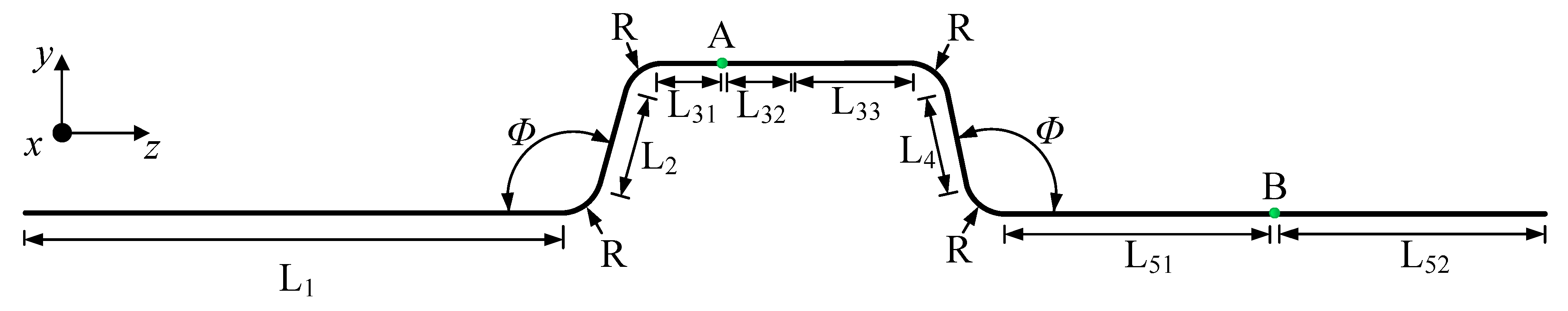
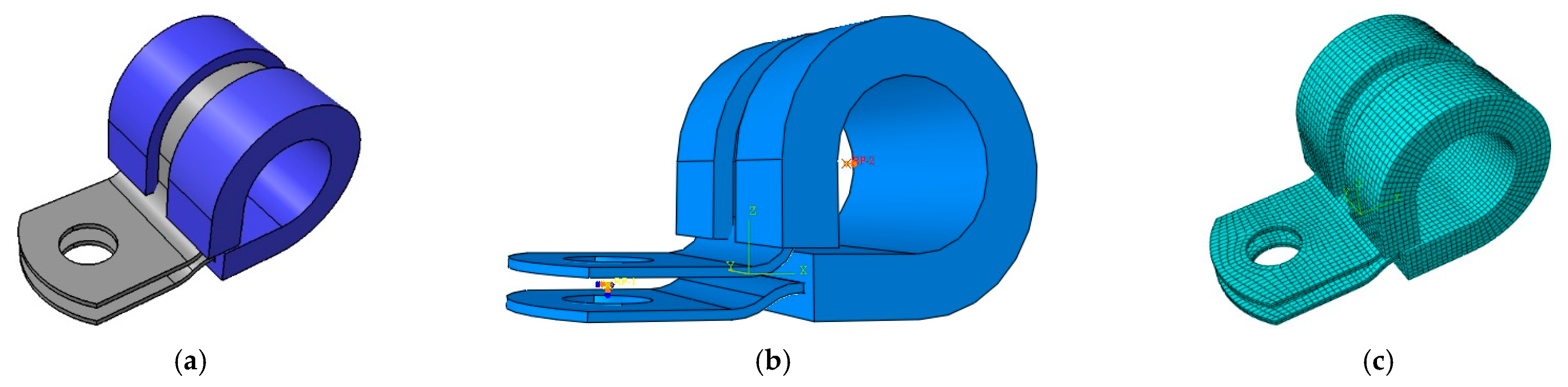
4.1. Aircraft Hydraulic Pipe Model

To validate the accuracy of the proposed methodology, the numerical solution and experiment of an ARJ21-700 aircraft hydraulic pipe with complex constraints is carried out. The pipe includes both straight pipe sections and elbow units, with a total of twelve parts, as shown schematically in Figure 2.

The overall transfer matrix of the pipe for numerical calculation is as follows:

$${\mathbf{U}}_{\mathrm{all}}={\mathbf{U}}_{L_{52}}{\mathbf{N}}_{A_2}{\mathbf{U}}_{L_{51}}{\mathbf{U}}_R{\mathbf{U}}_{L_4}{\mathbf{U}}_R{\mathbf{U}}_{L_{33}}{\mathbf{N}}_P{\mathbf{U}}_{L_{32}}{\mathbf{N}}_{A_1}{\mathbf{U}}_{L_{31}}{\mathbf{U}}_R{\mathbf{U}}_{L_2}{\mathbf{U}}_R{\mathbf{U}}_{L_1}$$

(44)

where ${\mathbf{N}}_{A1}$ and ${\mathbf{N}}_{A2}$ are the point transfer matrix, including the concentrated mass of accelerometer, and N_P is the point transfer matrix containing the concentrated mass and equivalent stiffness of the clamp.

Geometrical and material properties of the aircraft hydraulic pipe and fluid are listed in

Table 1. Geometrical and material properties of the aircraft hydraulic pipe and fluid.

Quantity	Symbol	Value	Unit	Quantity	Symbol	Value	Unit
pipe length	L1	534.261	mm	Bending angle	$\Phi$	1.649	rad
	L2	72.996	mm	Pipe density	${\rho }_p$	7760	kg/m3
	L31, L32	61.630	mm	Young’s modulus	E	190	GPa
	L33	123.260	mm	Poisson’s ratio	$\upsilon$	0.27	-
	L4	72.996	mm	Oil density	${\rho }_f$	872	kg/m3
	L51, L52	267.131	mm	Bulk modulus	Kf	1.95	GPa
outer diameter	D	9.525	mm	Kinematic viscosity	v	19.7	mm2/s
pipe wall thickness	e	0.889	mm	Transducer mass	ms	0.006	kg
bending radius	R	38.100	mm	Oil brand	10# aircraft hydraulic oil

.

4.2. Numerical Solution and Experimental Methods

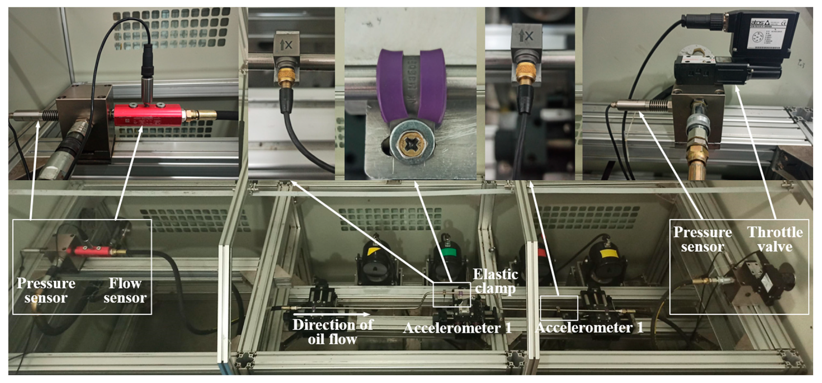
4.2.1. Experimental System

The schematic drawing of an experimental system for the aircraft hydraulic pipe is shown in Figure 3. The test pipe is connected with rubber hoses and fixed on the test bench at each end, and it is installed on the pipe bracket through an elastic clamp in the middle position. Hence, the boundary conditions at both ends of the pipe are simplified as fixed constraints, and the middle constraint of the pipe is the elastic support. The 7 piston swash plate type variable axial piston pump, with a displacement of 92 L/min, with a maximum working pressure that can approach 35 MPa, is adopted to regulate the system flow rate and meet the requirements of wide pressure and the Reynolds number range working conditions. The throttle valve is used to control the fluid pressure of the hydraulic pipeline system by adjusting the valve opening. The pressure sensor and flow sensor with high resolution are placed at both ends of the pipe to monitor fluid signals, and two lightweight acceleration sensors are placed at the pipe to collect vibration signals. The output signals are acquired and processed by a dynamic analyzer associated with a computer.

Figure 4 shows the experimental system and test bench layout, which mainly consists of five parts: the hydraulic pump station, test pipe and its component; sensor assembly and NI measurement system and data acquisition computer. The hydraulic pump station and measurement system are shown in Figure A1 (Appendix C). The detailed specification of the experimental equipment and measurement systems are listed in

Table A2. The specification of experimental apparatus and measurement system.

System	Item	Manufacturer/Type	Performance
Experimental apparatus	Axial piston pump	Rexroth A4VSO40DR10RPPB13N00N	Displacement: 92 L/min Pressure rating: 35 MPa
	Throttle valve	ATOS E-RI-TE-01H-41	Pressure range: 0~40 MPa
	Accelerometer	B&K BK4525-B-001	Measuring range: ±700 m/s2 Frequency range: 0–20 kHz
	Flow sensor	HYDAC EVS3104-A-0060-000	Measuring range: 6–60 L/min Output signal: 4–20 mA Measuring error: ≤2%
	Pressure sensor	Shanghai Dingwei Electronic Materials Co., Ltd. FST800-216G335C-400B	Measuring range: 0~40 MPa Output signal: 0–10 V Measuring error ≤: 0.5%
Measurement and control system	PXIe chassis	National Instruments PXIe-1078	9 AC hybrid slots System slot bandwidth: 250 MB/s System bandwidth: 1 GB/s
	PXIe controller	National Instruments PXIe-8820	Dual-core processor (2.2 GHz) System slot bandwidth: 250 MB/s System bandwidth: 1 GB/s
	Analog output card	National Instruments PXI-6723	32 analog output channels; Conversion rate: 10 kHz; Maximum sampling rate: 800 kS/s
	Data acquisition card	National Instruments PXI-6221	16 AI channels 2 AO channels Maximum sampling rate: 250 kS/s
	Vibration acquisition card	National Instruments PXIe-4497	24 channels 24 resolution Maximum sampling rate: 204.8 kS/s

(Appendix C).

4.2.2. System Work Conditions

In order to study the FSI vibration characteristics of the aircraft hydraulic pipe in wide pressure with the Reynolds number range, the flow and pressure are selected as design variables, and the four working conditions are designed.

The critical Reynolds number of the smooth pipe is [9]:

$$R{\mathrm{e}}_1=\frac{V_{1}D}{v}=2320$$

(45)

Through calculating, the critical flow velocity is $V_1=4.80\mathrm{m}/\mathrm{s}$. Therefore, the system flow velocity is set to 2 m/s (laminar flow) and 8 m/s (turbulent flow), respectively, and the system fluid pressure is set to 5 MPa and 10 MPa, respectively. Four system work conditions in this subsection are listed in

Table 2. Four system work conditions.

Work Conditions	Fluid Pressure (MPa)	Flow Velocity (m/s)	Flow Rate (L/min)	Reynolds Number	Flow Form
1	5	2	6.82	967.01	Laminar
2	5	8	27.3	3868.02	Turbulence
3	10	2	6.82	967.01	Laminar
4	10	8	27.3	3868.02	Turbulence

.

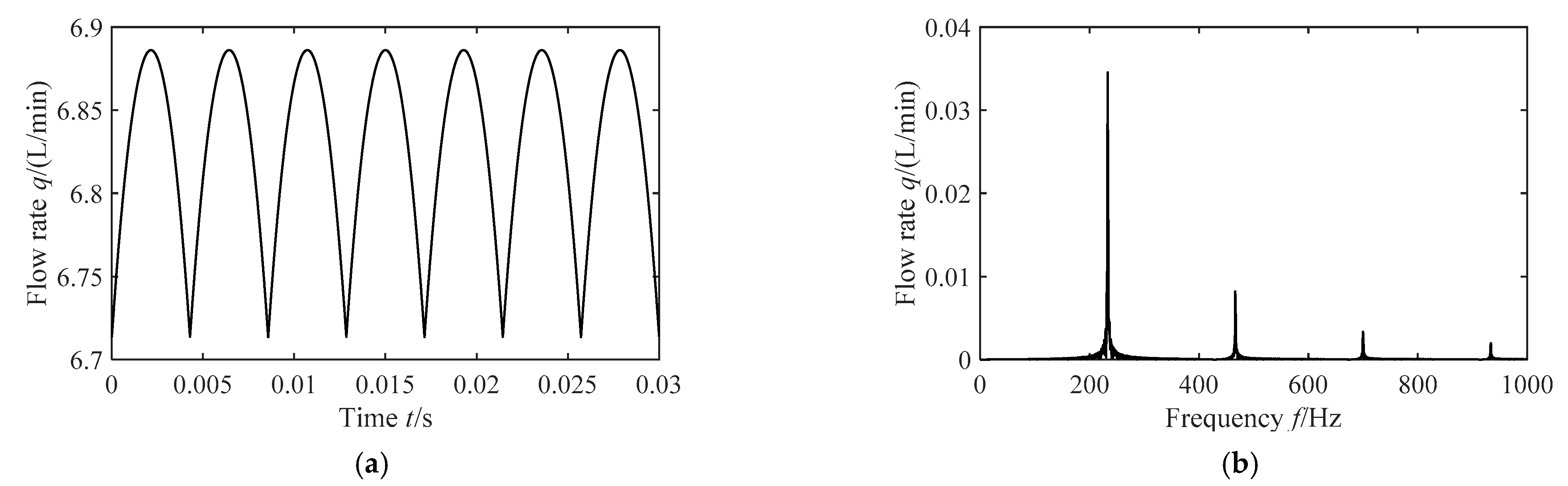
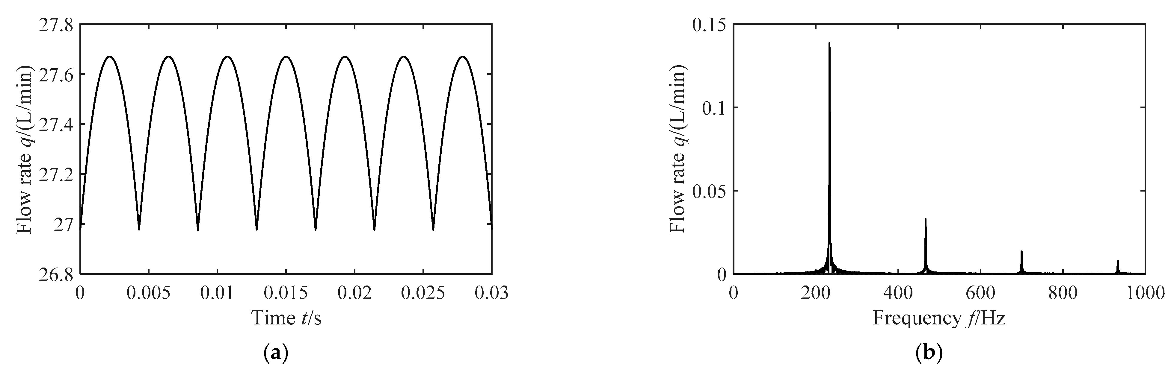
4.2.3. Flow Pulsation Excitation

The calculation and verification are carried out based on a seven pistons swash plate type variable axial piston pump; the instantaneous flow of piston pump could be expressed as:

$$\{\begin{array}{l}{q}_{sh}=AR\omega \tan \gamma \frac{\cos (\alpha /2-\phi )}{2\sin (\alpha /2)}(0\le \phi \le \alpha )\\ q_{sh}=AR\omega \tan \gamma \frac{\cos (3\alpha /2-\phi )}{2\sin (\alpha /2)}(\alpha \le \phi \le 2\alpha )\end{array}$$

(46)

where $2\alpha$ is the central angle between two adjacent plungers, $2\alpha =2\pi /z=2\pi /7$.

The rotational speed of the motor in the pumping plant is 1000 r/min, and the system flow rates are 6.82 L/min and 27.3 L/min, respectively; that is, the fluid velocities in the pipe are 2 m/s and 8 m/s. The flow pulsation of the axial piston pump is shown in Figure 5 and Figure 6.

According to the discussion about the excitation matrix model in Section 2.2, the first four-order harmonics of flow pulsation are used for calculating and studying. The first four-order spectrum characteristics of flow pulsation are listed in

Table 3. First four-order natural frequencies and amplitude of flow pulsation.

Flow Velocity (m/s)	f1 (Hz)	q1 (L/min)	f2 (Hz)	q2 (L/min)	f3 (Hz)	q3 (L/min)	f4 (Hz)	q4 (L/min)
2	227.8	0.03281	484.1	0.00594	711.9	0.00415	939.7	0.00270
8	227.8	0.13180	484.1	0.02390	711.9	0.01668	939.7	0.01083

.

According to $\omega =2\pi f$ and $V=Q/A_f$, the parameters of flow velocity can be calculated, as shown in

Table 4. Calculation parameters of flow velocity.

Flow Velocity (m/s)	${\mathit{\omega }}_1$	VA1 (m/s)	${\mathit{\omega }}_2$	VA1 (m/s)	${\mathit{\omega }}_3$	VA1 (m/s)	${\mathit{\omega }}_4$	VA1 (m/s)
2	1430.584	0.00851	3040.148	0.00154	4470.732	0.00108	5901.316	0.00070
8	1430.584	0.03418	3040.148	0.00620	4470.732	0.00433	5901.316	0.00281

.

The right end of the pipe is an opening valve and no external excitation. According to Equation (19), excitation vectors at both ends of the pipe can be expressed as:

$$\{\begin{array}{l}{\mathbf{Q}}_0={\left[\begin{array}{ccccccc}{V}_e& 0& 0& 0& 0& 0& 0\end{array}\right]}^{\mathrm{T}}\\ {\mathbf{Q}}_L={\left[\begin{array}{ccccccc}0& 0& 0& 0& 0& 0& 0\end{array}\right]}^{\mathrm{T}}\end{array}$$

(47)

4.2.4. Boundary Conditions

The boundary condition of the left end of the pipe is the velocity-inlet, which is the flow pulsation. The boundary condition of the right end of the pipe is the pressure-outlet, which is described by the linear characteristics of a throttle valve. The flow characteristics of the throttle valve can be expressed [45] as:

$$q=k_{q}A\Delta P^m$$

(48)

where q is the flow rate, k_q is the throttle coefficient, A is the throttle hole area and m is a parameter depending on the structure of the throttle valve. When there is linearity between the flow and pressure characteristics of the valve, m = 1, and the output pressure of the throttle valve is 0. Hence, a linear relationship between the flow and pressure characteristics of the pipe is as follows:

$$P=k_q(V-{\dot{\omega }}_z)$$

(49)

The throttle coefficients corresponding to the four system work conditions are listed in

Table 5. Throttle coefficient of four work conditions.

Work Conditions	Fluid Pressure (MPa)	Flow Velocity (m/s)	Flow Rate (L/min)	kq Pa/(m/s)
1	5	2	6.82	2.5 × 106
2	5	8	27.3	6.25 × 105
3	10	2	6.82	5 × 106
4	10	8	27.3	1.25 × 106

.

Both ends of the pipe are fixed and the stiffness factor of the support [19] is set to a maximum value (e¹²). The boundary matrices at both ends of the pipe are obtained according to Equations (A1) and (A2).

$${\mathbf{D}}_0=\left[\begin{array}{cccccccccccccc}1& 0& -1& 0& 0& 0& 0& 0& 0& 0& 0& 0& 0& 0\\ 0& -A_f& k_z\Delta t+\frac{m_0}{\Delta t}& 1& 0& 0& 0& 0& 0& 0& 0& 0& 0& 0\\ 0& 0& 0& 0& 0& 0& k_x\Delta t+\frac{m_0}{\Delta t}& 1& 0& 0& 0& 0& 0& 0\\ 0& 0& 0& 0& 1& 0& 0& 0& 0& 0& 0& 0& 0& 0\\ 0& 0& 0& 0& 0& 0& 0& 0& 0& 0& k_y\Delta t+\frac{m_0}{\Delta t}& 1& 0& 0\\ 0& 0& 0& 0& 0& 0& 0& 0& 0& 1& 0& 0& 0& 0\\ 0& 0& 0& 0& 0& 0& 0& 0& 0& 0& 0& 0& 0& 1\end{array}\right]$$

(50)

$${\mathbf{D}}_L=\left[\begin{array}{cccccccccccccc}-k_q& 1& k_q& 0& 0& 0& 0& 0& 0& 0& 0& 0& 0& 0\\ 0& -A_f& -(k_z\Delta t+\frac{m_L}{\Delta t})& 1& 0& 0& 0& 0& 0& 0& 0& 0& 0& 0\\ 0& 0& 0& 0& 0& 0& -(k_x\Delta t+\frac{m_L}{\Delta t})& 1& 0& 0& 0& 0& 0& 0\\ 0& 0& 0& 0& 1& 0& 0& 0& 0& 0& 0& 0& 0& 0\\ 0& 0& 0& 0& 0& 0& 0& 0& 0& 0& -(k_y\Delta t+\frac{m_L}{\Delta t})& 1& 0& 0\\ 0& 0& 0& 0& 0& 0& 0& 0& 0& 1& 0& 0& 0& 0\\ 0& 0& 0& 0& 0& 0& 0& 0& 0& 0& 0& 0& 0& 1\end{array}\right]$$

(51)

4.2.5. Middle Constraint

The HB3-25LB10B P-type clamp is used for analysis and verification, the P-type clamp is composed of a metal band and rubber washer, as shown in Figure 7a. For the numerical solution of the FSI model by the discrete time transfer matrix method, the middle constraint mainly contains stiffness, damping and added mass for numerical solution. The clamp mainly provides elastic constraints of translation and rotation, the translational stiffness and rotational stiffness are obtained through finite element method simulation, while the added mass is offset by the force provided by the test bench. The fastening effect of the P-type clamp is achieved by the outer surface extrusion of the rubber washer and pipeline. The bolt has little effect on the stiffness of the clamp, therefore, the bolt is neglected in the modeling process.

The Finite Element Analysis model of load setting is shown in Figure 7b, and uses the Cartesian coordinate system to indicate the axial, circumferential and radial directions. Using ABAQUS 6.14 finite element software, the model is meshed in fully structured hexahedron cells as shown in Figure 7c, which can effectively guarantee the simulation accuracy. The metal band material is 2A12 Aluminum Alloy and the constitutive model of clamp rubber washer material adopts the Mooney–Rivlin model;

Table 6. Material properties of the metal band and rubber washer.

	Material	Density (kg/m3)	Elastic Modulus (GPa)	Poisson’s Ratio
Metal band	Aluminium alloy (2A12)	2750	70	0.33
Rubber washer	Rubber (EPDM8370)	C10	C01	D0
		0.774	0.193	0.025

lists the related material properties.

In practice, the constraint between the metal band and rubber washer is set as binding, and there is no relative slide between them. The boundary condition of the bolt-hole in the metal band is set as fixed to limit the degrees of freedom of the clamp in six directions. First, coupling the inner surface of the metal band in contact with the pipe wall into a point and applying concentrated force or a moment at the coupling point, then, six-DOF equivalent stiffness of clamp can be obtained according to the linear displacement and angular displacement of the coupling point. The detailed solving methods and parameter settings are: the type of step is set to “static and general”, the geometric nonlinearity is turned on, the time period is set to one second, the minimum incremental step is set to 1 and the maximum incremental step is set to 100. The applied concentrated force is 1 N and the moment is 1N∙m. The six-DOF displacement results of the clamp are shown in Figure 8.

The six-DOF equivalent stiffness of clamp is listed in

Table 7. Six-DOF equivalent stiffness of clamp.

Translational Stiffness (N/m)			Rocking Stiffness (N∙m/rad)
kx	ky	kz	tx	ty	tz
8.74 × 106	5.84 × 105	7.29 × 106	1830	239	1890

, which is applied to the translation stiffness coefficient and rotational stiffness coefficient in Equation (25).

5. Results and Discussion

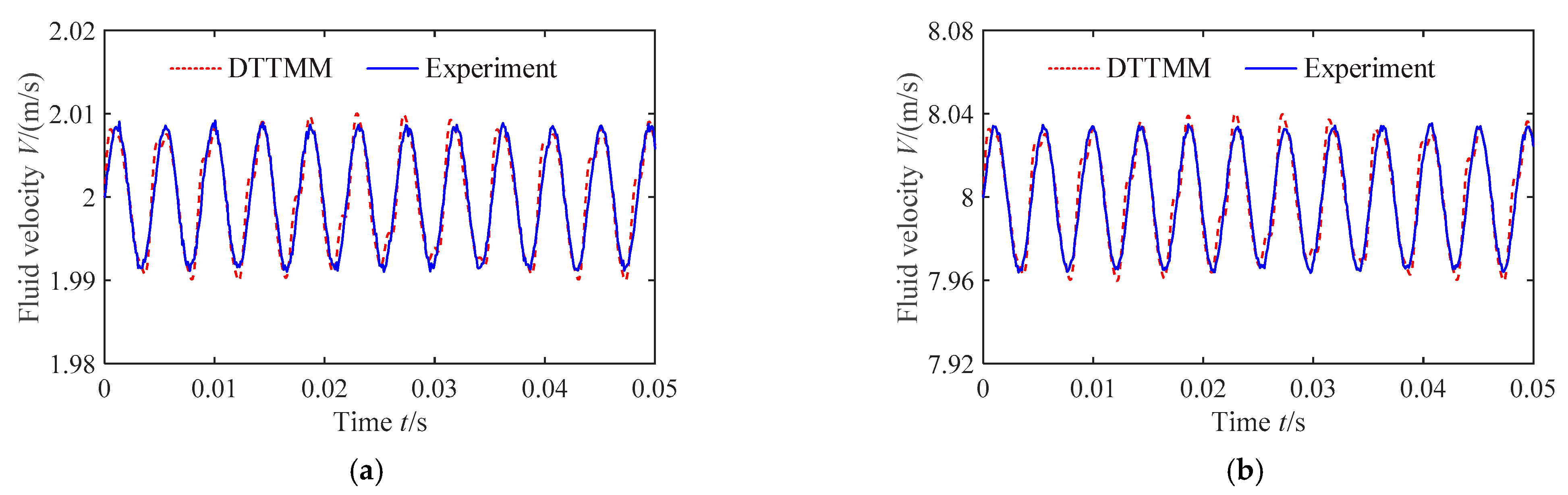
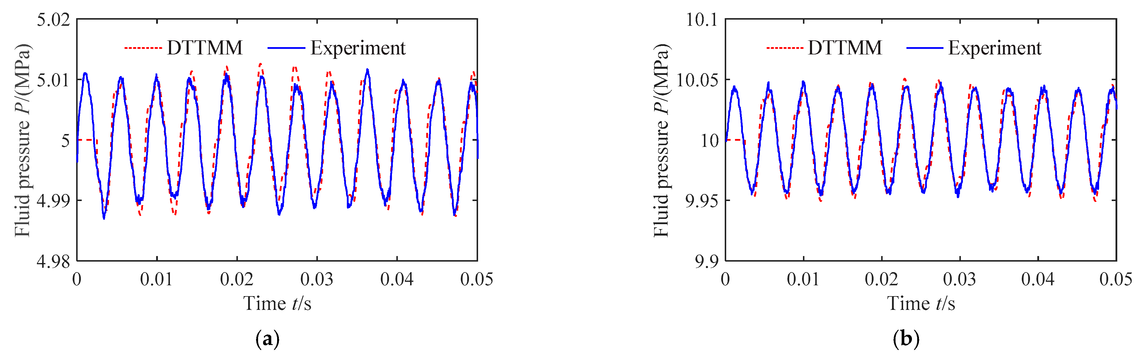
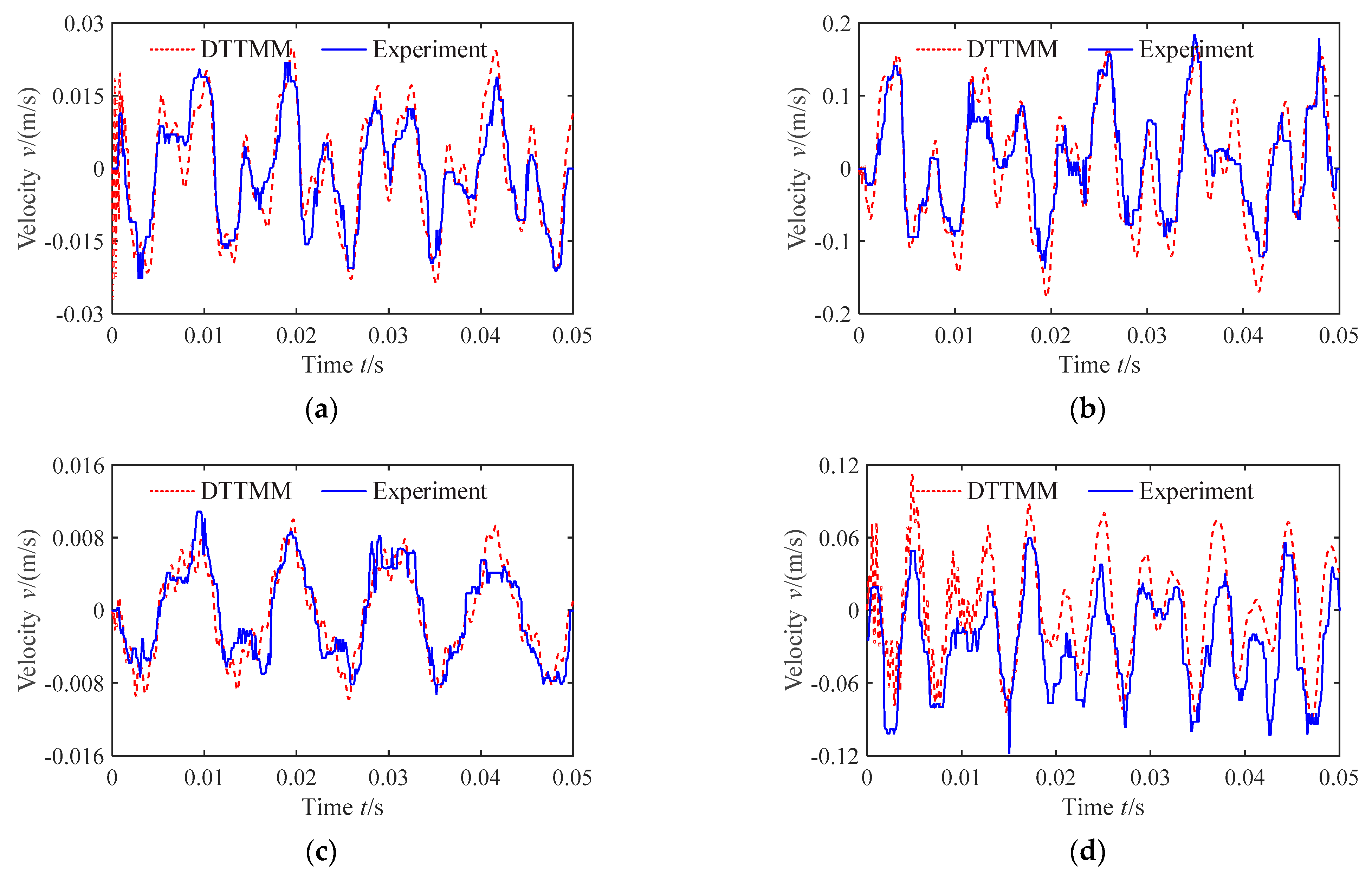
5.1. Dynamic Response Characteristics of Fluid

The dynamic response of fluid under four system work conditions (Table 2) is investigated in this subsection. The Figure 9 and Figure 10 show the comparison of the flow velocity at the inlet of the pipe and fluid pressure at the outlet of the pipe by the DTTMM method and the experimental results.

From Figure 9, it is observed that the flow velocity curves of the pipe inlet contain several sinusoidal components, show the periodic characteristics and the pulsating amplitude shows an increasing trend with increasing flow velocity. A key point here is that the waveform of flow velocity curves in Figure 9 is inconsistent with that in Figure 5a and Figure 6a; this is due to only the first four-order harmonics of pump source pulsation being used for calculation.

From Figure 10, it is observed that the fluid pressure curves of the pipe outlet contain several sinusoidal components, show the periodic characteristics and the pulsating amplitude increases with the increasing fluid pressure. Interestingly, the waveform of the fluid pressure curves in Figure 10 agrees with the flow velocity curves in Figure 9; this happens because the differential pressure and flow velocity across the throttle valve are defined as a linear relation in Equation (49). Moreover, it takes about two milliseconds for the fluid pressure pulsation to appear in the DTTMM method, while the pulsation phenomenon exists in the experimental results from the initial time. This is because, the initial state of the fluid in the pipe is static in the numerical simulation, and the pressure wave propagates at the speed of sound along the pipe. This time difference may be just the time of pressure wave from the head end to the tail end of the pipe exactly, while the experimental results are obtained when the test system is stable.

Figure 9 and Figure 10 show that there is a good agreement between the DTTMM method and the experimental results. However, the waveform amplitude of the experimental results is generally lower than that of the DTTMM method, principally because some hydraulic components, such as the accumulator and filter, are installed in the experimental system, which will absorb part of the fluid pulsation; however, those components are not modeled and analyzed in the numerical calculation.

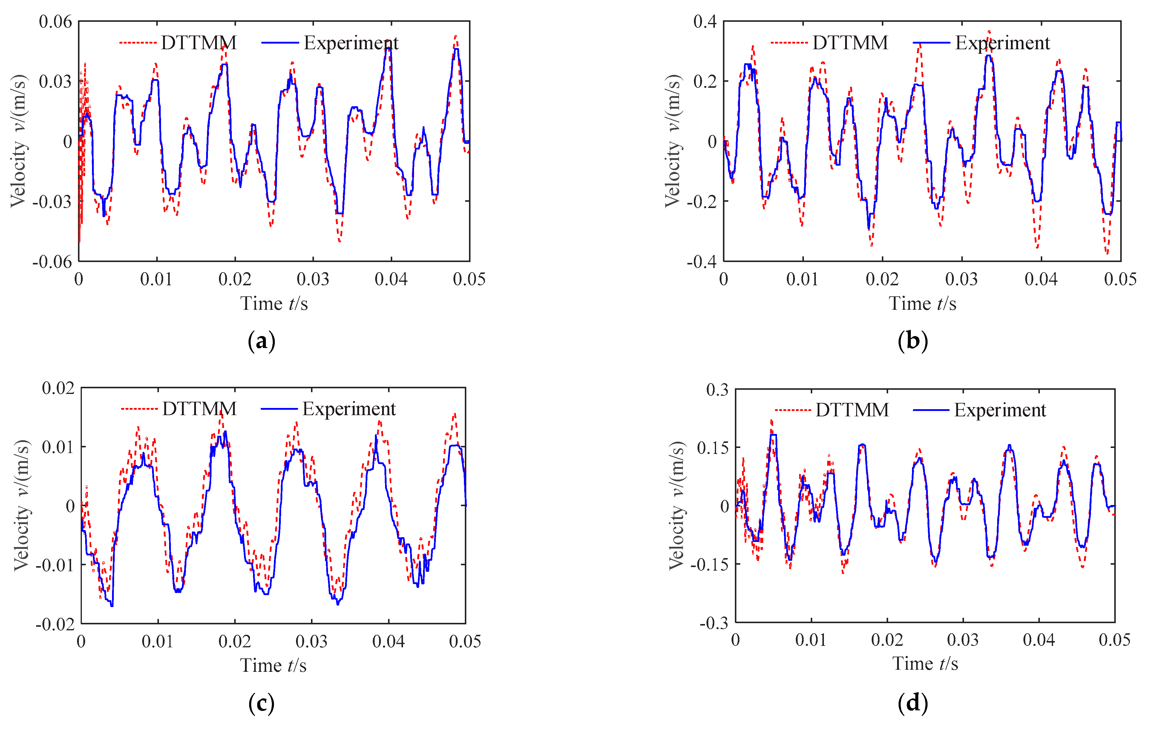
5.2. Dynamic Response Characteristics of Pipes

The dynamic response of the pipe under four system work conditions (Table 2) is investigated in this subsection. Figure 11, Figure 12, Figure 13 and Figure 14 shows the comparison of vibration velocity of measuring points A and B in the pipe by the DTTMM method and the experimental results.

From Figure 11, Figure 12, Figure 13 and Figure 14, it is observed that the vibration response of the pipe under the flow pulsation excitation shows a forced vibration with periodic characteristics, and the vibration velocity response law of pipe is consistent with the variation law of fluid pulsation. The radial vibration response amplitude is generally higher than the axial vibration response amplitude, suggesting that the flow pulsation excitation will cause a large amplitude radial vibration of pipe.

Comparing the velocity response of the pipe measuring points under different working conditions, it can be concluded that the vibration amplitude increases with the increasing flow velocity when the system pressure is constant. The waveform of vibration velocity response curves changes as well; it appears as the higher the flow velocity, the earlier the vibration velocity reaches the response peak. Moreover, when the flow velocity is constant, the vibration amplitude increases with the increasing system pressure, but the variation amplitude is relatively smaller, indicating that the fluid pressure has relatively less influence on the vibration velocity of the pipe.

From Figure 11, Figure 12, Figure 13 and Figure 14, we can see that the DTTMM results are in good agreement with the experimental results. However, compared with the theoretical predictions (DTTMM method), the waveform of the experimental curves has more small clutter and the vibration response amplitude is generally lower.

The little disparity between theory and experiment may be caused by the following reasons:

• Calculation error of theoretical results from analytical approximations and numerical error, etc.
• There are manufacturing error and installation deviation in the manufacturing and installation process of the test pipe.
• The textile-reinforced rubber hoses and elastic clamps exist in the experimental system, which will increase the damping characteristics of the system, but the damping dissipation of the above components is neglected in numerical calculation.
• There are measurement noises in the process of data acquisition, such as sensor noise, supply line noise and signal line noise, etc.

6. Conclusions

The FSI response characteristics of aircraft hydraulic pipe with complex constraints and boundary conditions are studied in this paper. The main work and research conclusions are as follows.

• The FSI fourteen-equation theoretical model of pipe conveying fluid is developed. The modified friction coupling model is contained in the axial motion equations, and the impacts of gravity, centrifugal force, Coriolis force and the moment of inertia caused by the fluid within the pipe, takes into account in the method that is applicable for describing the FSI of pipe conveying fluid in wide pressure and Reynolds number range.
• The external excitation model, boundary condition model and middle constraint are developed for solving the FSI fourteen-equation model. These models contain the flow pulsation excitation of axial piston pump, the velocity-inlet boundary condition, pressure-outlet boundary condition and the middle constraint (elastic clamp), which can be applied to solve the complex hydraulic pipeline system with various fluid and structural excitation, when complex constraints are contained.
• A discrete time transfer matrix method (DTTMM) for solving the FSI fourteen-equation model in time domain is presented. The excellent feature of the present method is that the whole solution procedure can be independently described by a unified matrix expression. It means that there is not any modification to the solution procedures from one analysis model to another, which makes a stylization solution method and further comprehensive investigation easier compared to most existing solution methods.
• The numerical solution and experiment of an ARJ21-700 aircraft hydraulic pipe with complex constraints are carried out under four working conditions to prove the theoretical model and solution method presented in this work. The results calculated by the DTTMM method are in good agreement with the experimental data, and the research shows that the pulsating amplitude of fluid increases with the increasing flow velocity and fluid pressure. As for the pipe, the vibration response under the flow pulsation excitation shows a forced vibration with periodic characteristics, and the flow pulsation excitation will cause large amplitude radial vibration of pipe. Moreover, the vibration amplitude increases with the increasing flow velocity, and the higher the flow velocity is, the earlier the vibration velocity reaches the response peak, but the fluid pressure has relatively less influence on the vibration response.

The proposed methodology can be successfully used for the analysis of the FSI response characteristics of the aircraft hydraulic pipe with complex constraints and boundary conditions, which can also provide theoretical references and engineering technology guidance for the FSI analysis of pipe conveying fluid. Further work will involve the frequency domain analyses and the investigation of a complete aircraft hydraulic pipeline system.

7. Patents

Invention patent: Performance test experiment platform and its test methods of the high-pressure aircraft hydraulic pipe.

Patent number: ZL202110492169.3

Software copyright: (1) Simulation and analysis software platform for Fluid-structure interaction vibration characteristics of the aircraft hydraulic pipe. (2) Modal Analysis software platform of aircraft hydraulic pipe.

Registration number: 2020SR1135782 and 2020SR1135790.

References

1. Gao, P.; Yu, T.; Zhang, Y.; Wang, J.; Zhai, J. Vibration analysis and control technologies of hydraulic pipeline system in aircraft: A review. Chin. J. Aeronaut. 2021, 34, 83–114. [Google Scholar] [CrossRef]
2. Zhang, Y.; Liu, X.; Rong, W.; Gao, P.; Yu, T.; Han, H.; Xu, L. Vibration and Damping Analysis of Pipeline System Based on Partially Piezoelectric Active Constrained Layer Damping Treatment. Materials 2021, 14, 1209. [Google Scholar] [CrossRef]
3. Song, X.; Cao, T.; Gao, P.; Han, Q. Vibration and damping analysis of cylindrical shell treated with viscoelastic damping materials under elastic boundary conditions via a unified Rayleigh-Ritz method. Int. J. Mech. Sci. 2020, 165, 105158. [Google Scholar] [CrossRef]
4. Gao, P.; Li, J.; Zhai, J.; Tao, Y.; Han, Q. A Novel Optimization Layout Method for Clamps in a Pipeline System. Appl. Sci. 2020, 10, 390. [Google Scholar] [CrossRef] [Green Version]
5. Zhai, J.; Li, J.; Wei, D.; Gao, P.; Yan, Y.; Han, Q. Vibration Control of an Aero Pipeline System with Active Constraint Layer Damping Treatment. Appl. Sci. 2019, 9, 2094. [Google Scholar] [CrossRef] [Green Version]
6. Yan, Y.; Zhai, J.; Gao, P.; Han, Q. A multi-scale finite element contact model for seal and assembly of twin ferrule pipeline fittings. Tribol. Int. 2018, 125, 100–109. [Google Scholar] [CrossRef]
7. Wang, M.; Jiao, Z.; Xu, Y. Analytical method of thermal-fluid transients in aerohydraulic systems. In Proceedings of the 2015 International Conference on Fluid Power and Mechatronics, Haerbin, China, 14–15 September 2015; pp. 63–67. [Google Scholar]
8. Li, Y.; Jiao, Z.; Xu, Y. Nonlinear Analysis of Oscillations in Aero-hydraulic Actuation System Considering Load Effect. In Proceedings of the 2015 International Conference on Fluid Power and Mechatronics 2015, Haerbin, China, 14–15 September 2015; pp. 934–938. [Google Scholar]
9. Quan, L.; Che, S.; Guo, C.; Gao, H.; Guo, M. Axial Vibration Characteristics of Fluid-Structure Interaction of an Aircraft Hydraulic Pipe Based on Modified Friction Coupling Model. Appl. Sci. 2020, 10, 3548. [Google Scholar] [CrossRef]
10. Zhang, Q.; Kong, X.; Huang, Z.; Yu, B.; Meng, G. Fluid-Structure-Interaction Analysis of an Aero Hydraulic Pipe Considering Friction Coupling. IEEE Access 2019, 7, 26665–26677. [Google Scholar] [CrossRef]
11. Joukowsky, N. On the hydraulic hammer in water supply pipes. Proc. Am. Water Works Assoc. 1904, 24, 341–424. [Google Scholar]
12. Skalak, R. An extension of the theory of water hammer. Trans. ASME 1956, 78, 105–116. [Google Scholar]
13. Wiggert, D.C.; Otwell, R.S.; Hatfield, F.J. The Effect of Elbow Restraint on Pressure Transients. J. Fluid. Eng. 1985, 107, 402–406. [Google Scholar] [CrossRef]
14. You, J.H.; Inaba, K. Fluid-structure interaction in water-filled thin pipes of anisotropic composite materials. J. Fluid. Struct. 2013, 36, 162–173. [Google Scholar] [CrossRef]
15. Walker, J.S.; Phillips, J.W. Pulse propagation in fluid-filled tubes. J. Press. Vess. Technol. ASME 1977, 77, 31–35. [Google Scholar] [CrossRef]
16. Davidson, L.C. Liquid-Structure Coupling in Curved Pipes. Shock Vib. Bull. 1969, 40, 197–207. [Google Scholar]
17. Wiggert, D.C.; Tijsseling, A.S. Fluid transients and fluid-structure interaction in flexible liquid-filled piping. Appl. Mech. Rev. 2001, 54, 455–481. [Google Scholar] [CrossRef]
18. Liu, G.; Li, S.; Li, Y.; Chen, H. Vibration analysis of pipelines with arbitrary branches by absorbing transfer matrix method. J. Sound Vib. 2013, 332, 6519–6536. [Google Scholar] [CrossRef]
19. Xu, Y.; Johnston, D.N.; Jiao, Z.; Plummer, A.R. Frequency modelling and solution of fluid-structure interaction in complex pipelines. J. Sound Vib. 2014, 333, 2800–2822. [Google Scholar] [CrossRef] [Green Version]
20. Lesmez, M.W.; Wiggert, D.C.; Hatfield, F.J. Modal Analysis of Vibrations in Liquid-Filled Piping Systems. J. Fluid. Eng. 1990, 112, 311–318. [Google Scholar] [CrossRef]
21. Zhang, L.; Tijsseling, S.A.; Vardy, E.A. Fsi Analysis of Liquid-Filled Pipes. J. Sound Vib. 1999, 224, 69–99. [Google Scholar] [CrossRef] [Green Version]
22. Hatfield, F.J.; Wiggert, D.C.; Otwell, R.S. Fluid Structure Interaction in Piping by Component Synthesis. J. Fluid. Eng. 1982, 104, 318–325. [Google Scholar] [CrossRef]
23. Zhang, X.M. Parametric studies of coupled vibration of cylindrical pipes conveying fluid with the wave propagation approach. Comput. Struct. 2002, 80, 287–295. [Google Scholar] [CrossRef]
24. Burmann, W. Water hammer in coaxial pipe system. ASCE J. Hydraul. Div. 1975, 101, 699–715. [Google Scholar] [CrossRef]
25. Hu, C.K.; Phillips, J.W. Pulse Propagation in Fluid-Filled Elastic Curved Tubes. J. Press. Vess.-Technol. ASME 1981, 103, 43–49. [Google Scholar] [CrossRef]
26. Ellis, J. A study of pipe-liquid interaction following pump trip and check-valve closure in a pumping station. In Proceedings of the 3rd International Conference on Pressure Surges, Canterbury, UK, 25–27 March 1980; pp. 203–220. [Google Scholar]
27. Ruoff, J.; Hodapp, M.; Kück, H. Finite element modelling of Coriolis mass flowmeters with arbitrary pipe geometry and unsteady flow conditions. Flow Meas. Instrum. 2014, 37, 119–126. [Google Scholar] [CrossRef]
28. Sreejith, B.; Jayaraj, K.; Ganesan, N.; Padmanabhan, C.; Chellapandi, P.; Selvaraj, P. Finite element analysis of fluid-structure interaction in pipeline systems. Nucl. Eng. Des. 2004, 227, 313–322. [Google Scholar] [CrossRef]
29. Zhang, Y.L.; Gorman, D.G.; Reese, J.M. A finite element method for modelling the vibration of initially tensioned thin-walled orthotropic cylindrical tubes conveying fluid. J. Sound Vib. 2001, 245, 93–112. [Google Scholar] [CrossRef]
30. Achouyab, E.H.; Bahrar, B. Numerical modeling of phenomena of waterhammer using a model of fluid-structure interaction. Comptes Rendus Mec. 2011, 339, 262–269. [Google Scholar] [CrossRef]
31. Ahmadi, A.; Keramat, A. Investigation of fluid-structure interaction with various types of junction coupling. J. Fluid. Struct. 2010, 26, 1123–1141. [Google Scholar] [CrossRef]
32. Wiggert, D.C.; Hatfield, F.J.; Stuckenbruck, S. Analysis of Liquid and Structural Transients in Piping by the Method of Characteristics. J. Fluid. Eng. 1987, 109, 161–165. [Google Scholar] [CrossRef]
33. Tijsseling, A.S. Fluid-Structure Interaction in Case of Waterhammer with Cavitation. Ph.D. Thesis, Delft University of Technology, Delft, The Netherlands, 1993. [Google Scholar]
34. Ouyang, X.; Gao, F.; Yang, H.; Wang, H. Two-dimensional stress analysis of the aircraft hydraulic system pipeline. Proc. Inst. Mech. Eng. Part G J. Aerosp. Eng. 2011, 226, 532–539. [Google Scholar] [CrossRef]
35. Tentarelli, S.C. Propagation of Noise and Vibration in Complex Hydraulic Tubing Systems. Ph.D. Thesis, Lehigh University, Bethlehem, PA, USA, 1990. [Google Scholar]
36. Gale, J.; Tiselj, I. Eight equation model for arbitrary shaped pipe conveying fluid. In Proceedings of the International Conference Nuclear Energy for New Europe, Portoroz, Slovenia, 18–21 September 2006. [Google Scholar]
37. Guan, C.; Jiao, Z.; He, S. Theoretical study of flow ripple for an aviation axial-piston pump with damping holes in the valve plate. Chin. J. Aeronaut. 2014, 27, 169–181. [Google Scholar] [CrossRef] [Green Version]
38. Bahr, M.K.; Svoboda, J.; Bhat, R.B. Vibration analysis of constant power regulated swash plate axial piston pumps. J. Sound Vib. 2003, 259, 1225–1236. [Google Scholar] [CrossRef]
39. Tijsseling, A.S. Fluid-Structure Interaction and Cavitation in a Single-Elbow Pipe System. J. Fluid. Struct. 1996, 10, 395–420. [Google Scholar] [CrossRef]
40. Budny, D.D.; Wiggert, D.C.; Hatfield, F.J. The Influence of Structural Damping on Internal Pressure during a Transient Pipe Flow. J. Fluid. Eng. 1991, 113, 424–429. [Google Scholar] [CrossRef]
41. Kwong, A.; Edge, K.A. A method to reduce noise in hydraulic systems by optimizing pipe clamp locations. Proc. Inst. Mech. Eng. J. Syst. Control Eng. 1998, 212, 267–280. [Google Scholar] [CrossRef]
42. Wu, J.-S.; Shih, P.Y. The dynamic analysis of a multispan fluid-conveying pipe subjected to external load. J. Sound Vib. 2001, 239, 201–215. [Google Scholar] [CrossRef]
43. Ke, Y.; Li, Q.S.; Zhang, L. Longitudinal vibration analysis of multi-span liquid-filled pipelines with rigid constraints. J. Sound Vib. 2004, 273, 125–147. [Google Scholar]
44. Xu, Y.; Jiao, Z. Exact solution of axial liquid-pipe vibration with time-line interpolation. J. Fluid. Struct. 2017, 70, 500–518. [Google Scholar] [CrossRef]
45. Gao, P.X.; Zhai, J.Y.; Han, Q.K. Dynamic response analysis of aero hydraulic pipeline system under pump fluid pressure fluctuation. Proc. Inst. Mech. Eng. 2019, 233, 1585–1595. [Google Scholar] [CrossRef]
Figure 1. Coordinate system of the fluid-filled pipe section.
Applsci 11 11918 g001
Figure 2. Schematic drawing of the ARJ21-700 aircraft hydraulic pipe.
Applsci 11 11918 g002
Figure 3. Schematic drawing of experimental system.
Applsci 11 11918 g003
Figure 4. Photograph of experimental platform.
Applsci 11 11918 g004
Figure 5. Flow pulsation curves of axial piston pump (The flow velocity is 2 m/s). (a) Pulsation curve in time domain; (b) Pulsation curve in frequency domain.
Applsci 11 11918 g005
Figure 6. Flow pulsation curves of axial piston pump (The flow velocity is 8 m/s). (a) Pulsation curve in time domain; (b) Pulsation curve in frequency domain.
Applsci 11 11918 g006
Figure 7. Finite element model of clamp and analysis settings. (a) Finite element model; (b) Constraints and loads; (c) Meshing result.
Applsci 11 11918 g007
Figure 8. Six-DOF displacement results of the clamp. (a) Linear displacement in the x-direction; (b) Linear displacement in the y-direction; (c) Linear displacement in the z-direction; (d) Angular displacement in the x-direction.; (e) Angular displacement in the y-direction; (f) Angular displacement in the z-direction.
Applsci 11 11918 g008
Figure 9. Flow velocity of pipe inlet. (a) Work conditions 1 and 3; (b) Work conditions 2 and 4.
Applsci 11 11918 g009
Figure 10. Fluid pressure of pipe outlet. (a) Work conditions 1 and 2; (b) Work conditions 3 and 4.
Applsci 11 11918 g010
Figure 11. Vibration velocity of pipe (the first condition). (a) Axial vibration velocity of measuring point A; (b) Radial vibration velocity of measuring point A; (c) Axial vibration velocity of measuring point B; (d) Radial vibration velocity of measuring point B.
Applsci 11 11918 g011
Figure 12. Vibration velocity of pipe (the second condition). (a) Axial vibration velocity of measuring point A; (b) Radial vibration velocity of measuring point A; (c) Axial vibration velocity of measuring point B; (d) Radial vibration velocity of measuring point B.
Applsci 11 11918 g012
Figure 13. Vibration velocity of pipe (the third condition). (a) Axial vibration velocity of measuring point A; (b) Radial vibration velocity of measuring point A; (c) Axial vibration velocity of measuring point B; (d) Radial vibration velocity of measuring point B.
Applsci 11 11918 g013
Figure 14. Vibration velocity of pipe (the fourth condition). (a) Axial vibration velocity of measuring point A; (b) Radial vibration velocity of measuring point A; (c) Axial vibration velocity of measuring point B; (d) Radial vibration velocity of measuring point B.
Applsci 11 11918 g014