
Numerical Study of the Unsteady Aerodynamic Performance of Two Maglev Trains Passing Each Other in Open Air Using Different Turbulence Models

Abstract
1. Introduction
2. Methodology
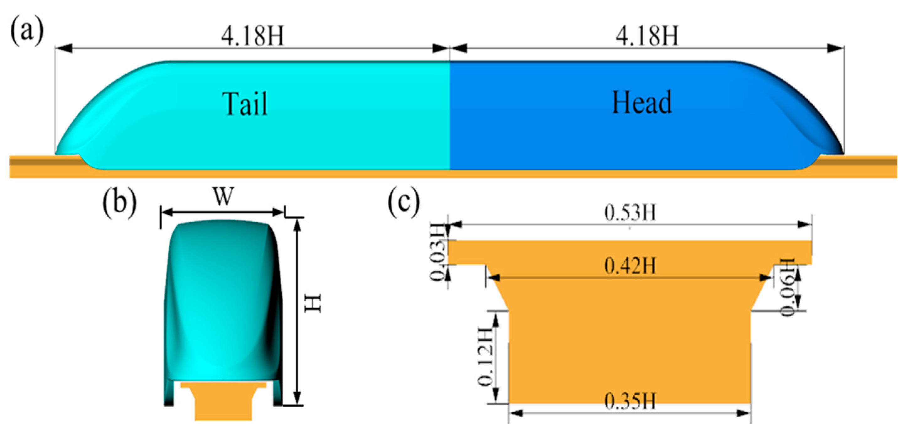
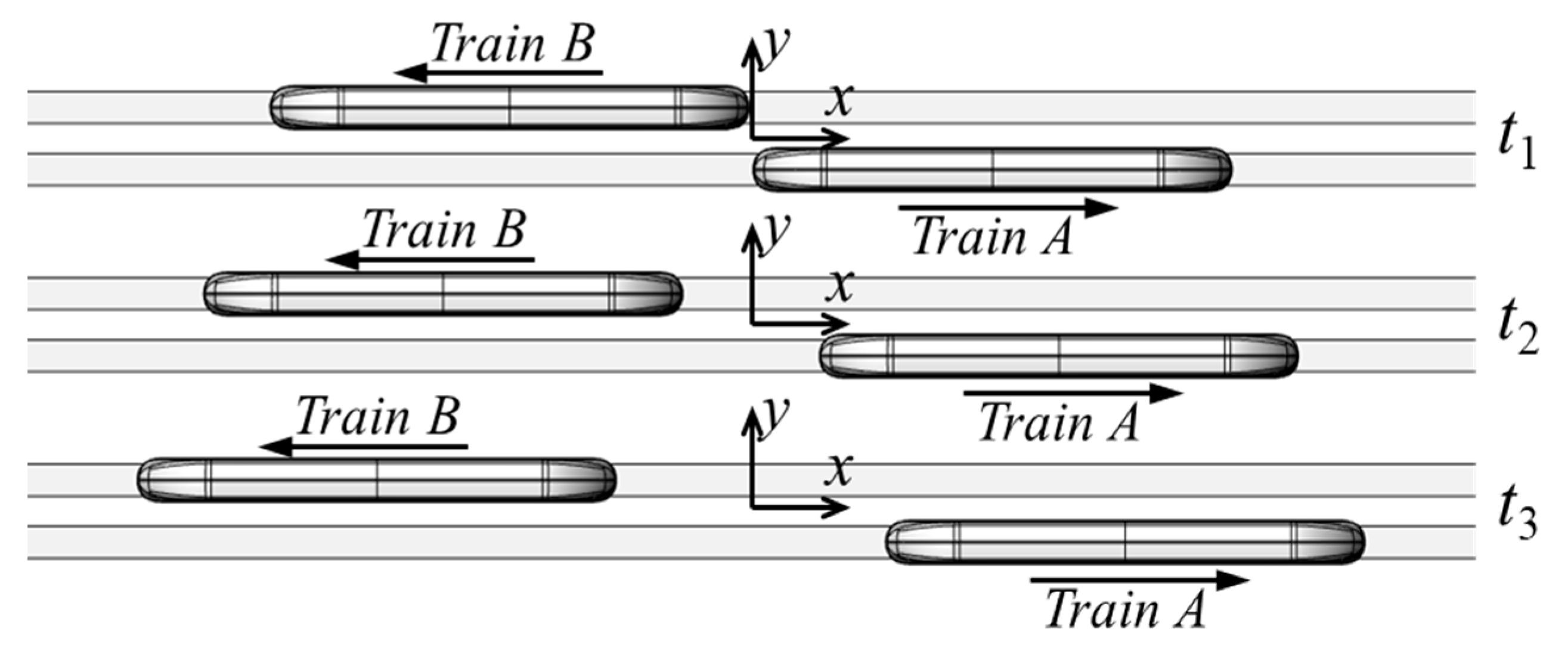
2.1. Geometry Model
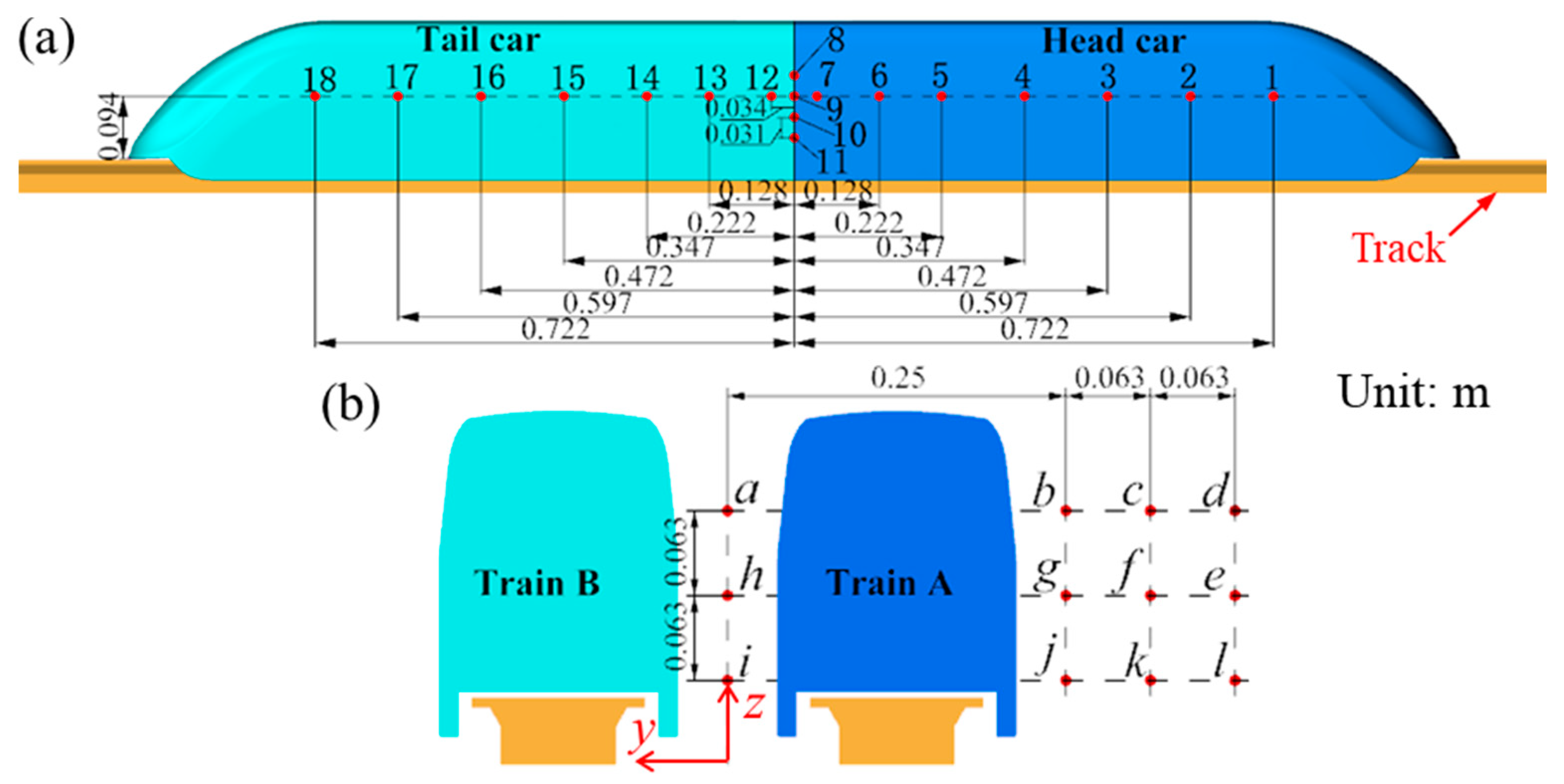
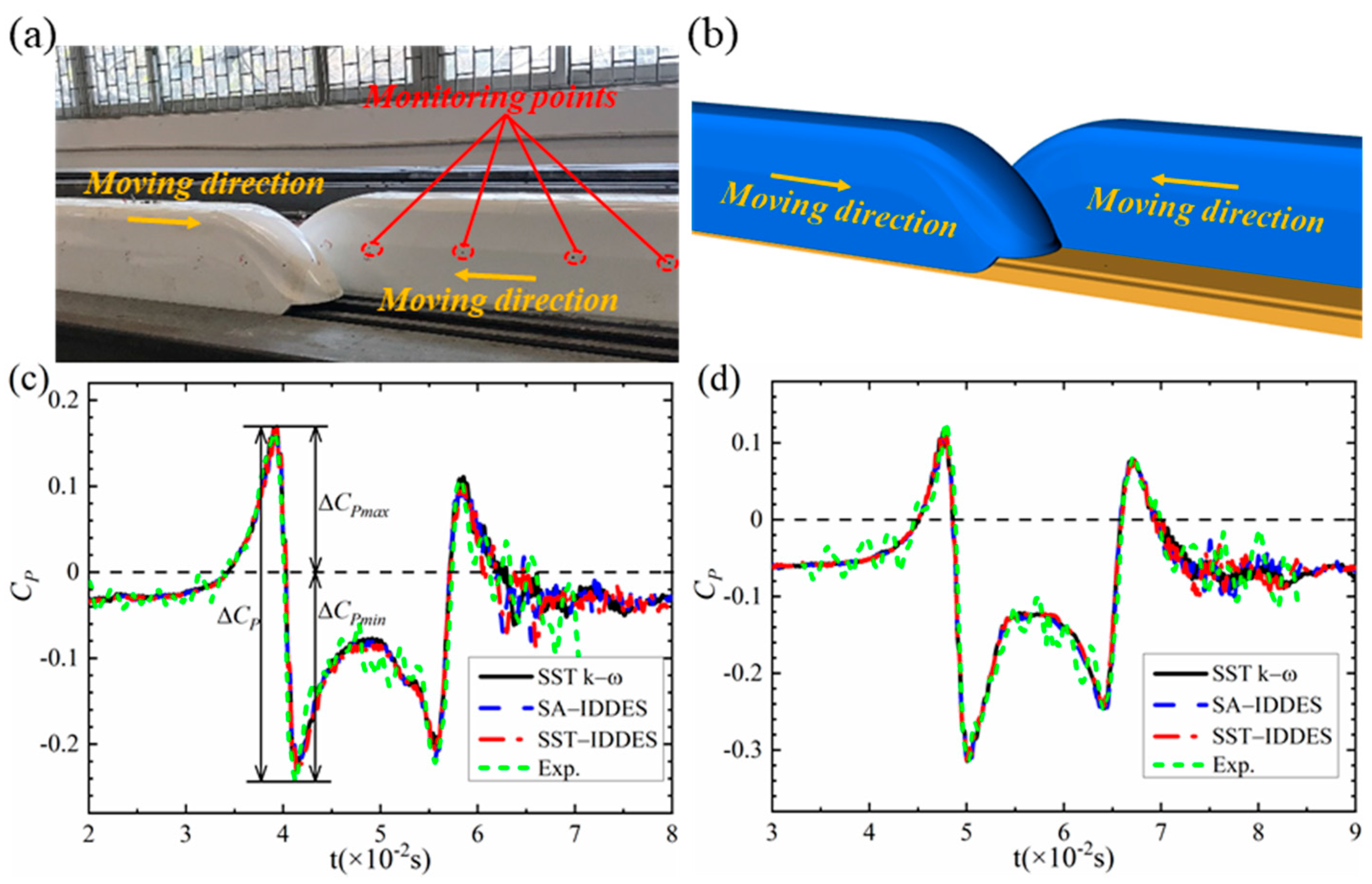
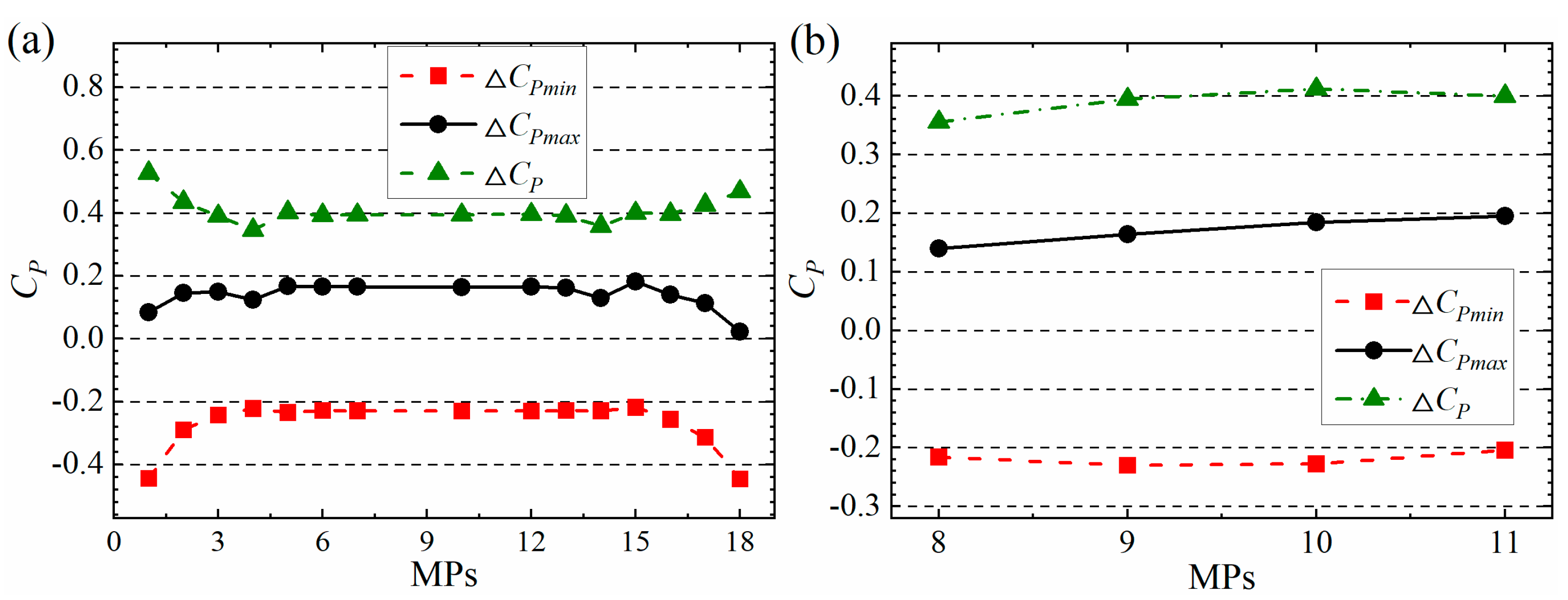
2.2. Monitoring Points
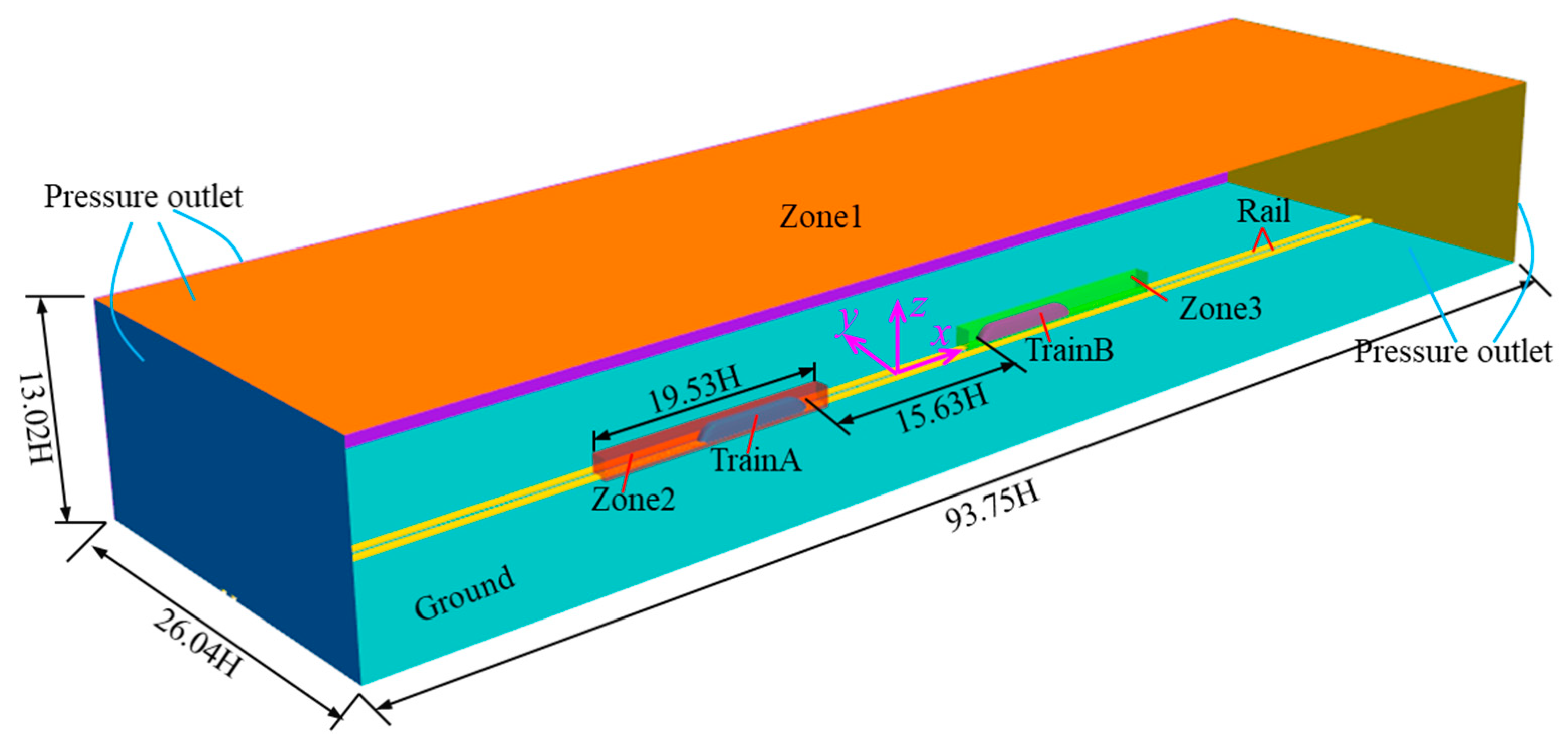
2.3. Computational Domain and Boundary Conditions
2.4. Numerical Method
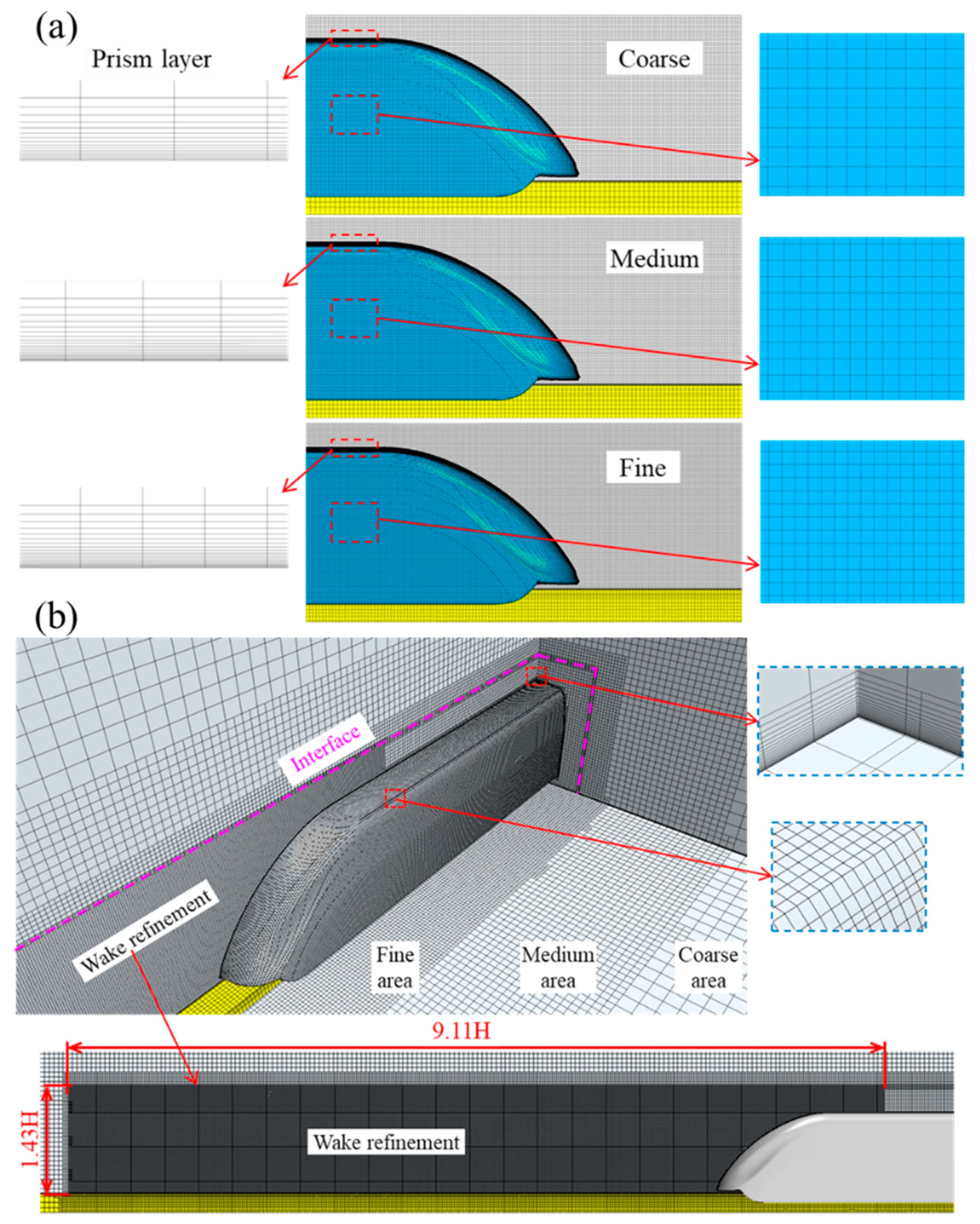
2.5. Mesh Generation
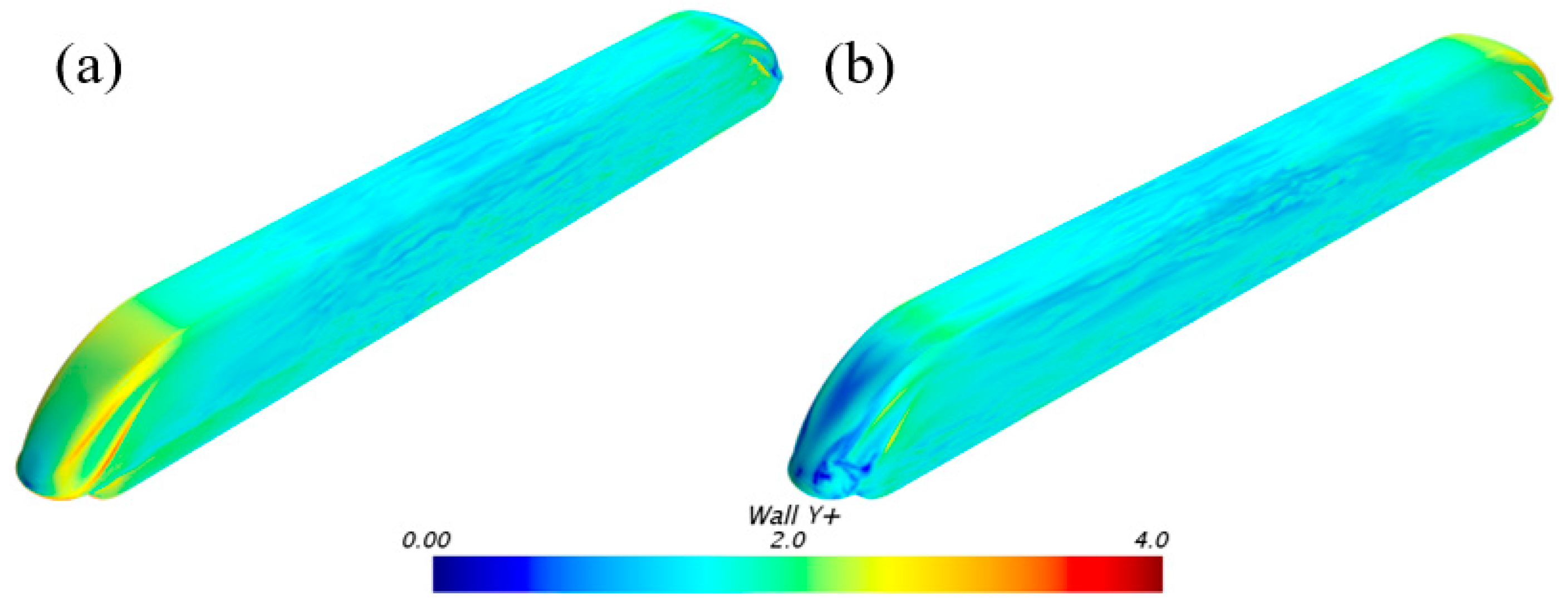
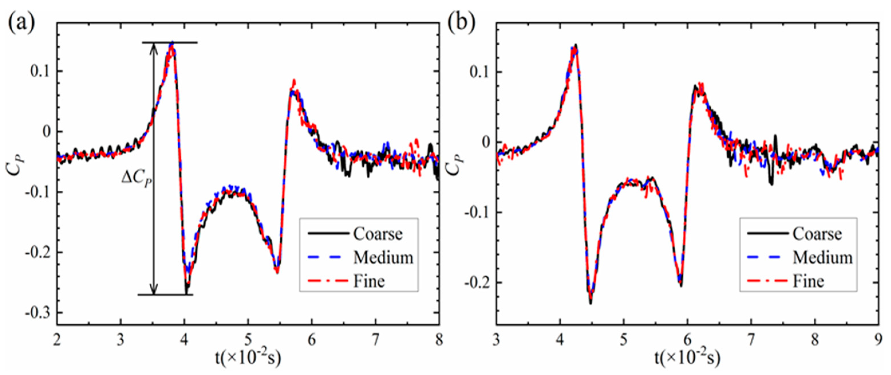
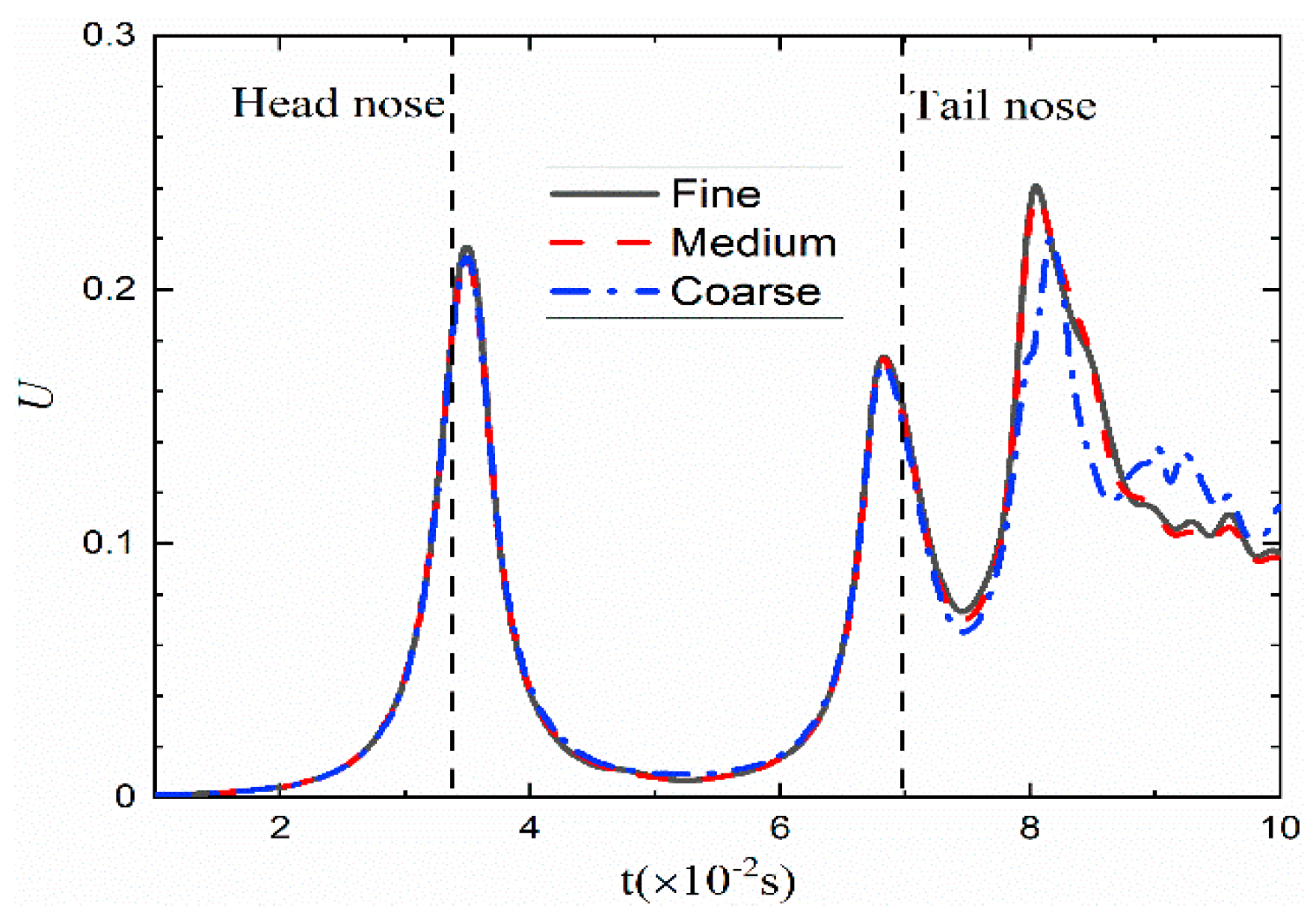
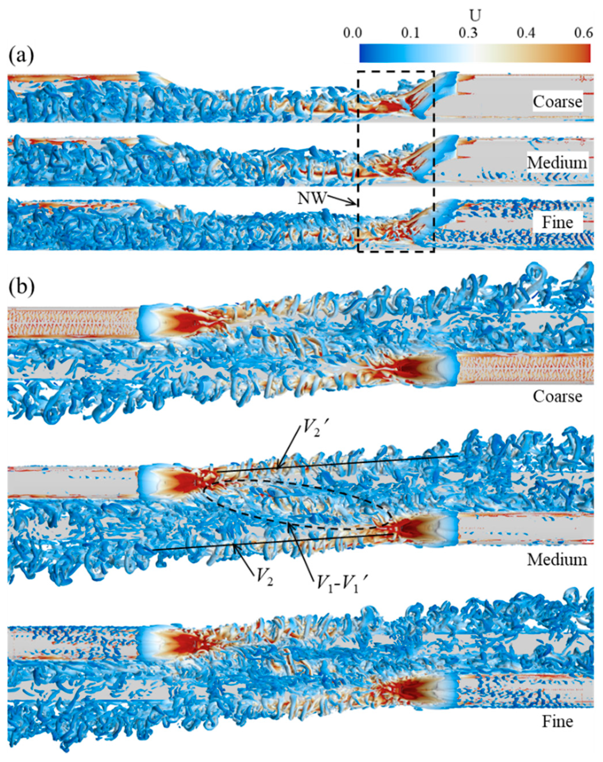
2.6. Mesh Sensitivity
3. Results and Discussion
3.1. Experimental Validation and Transient Pressure
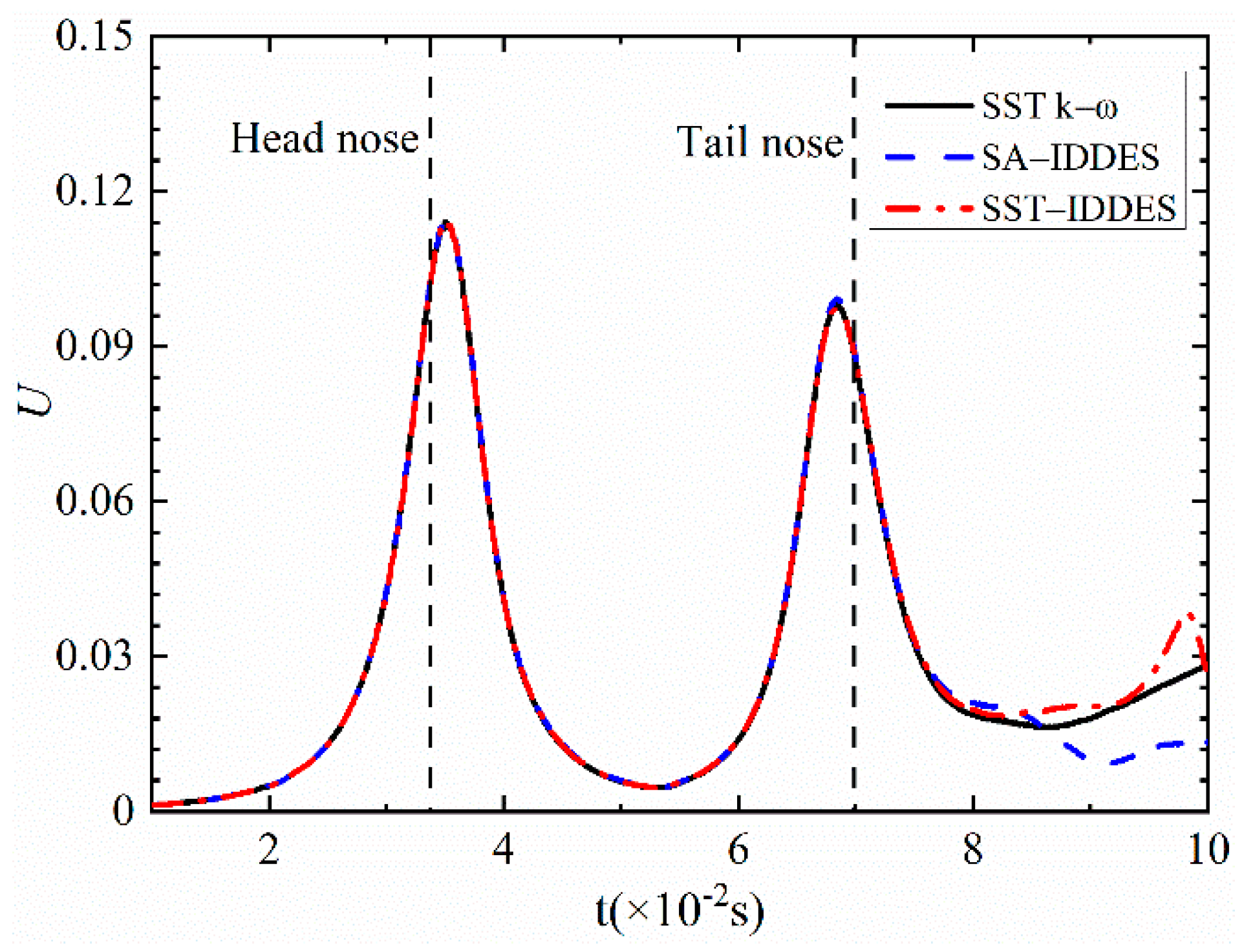
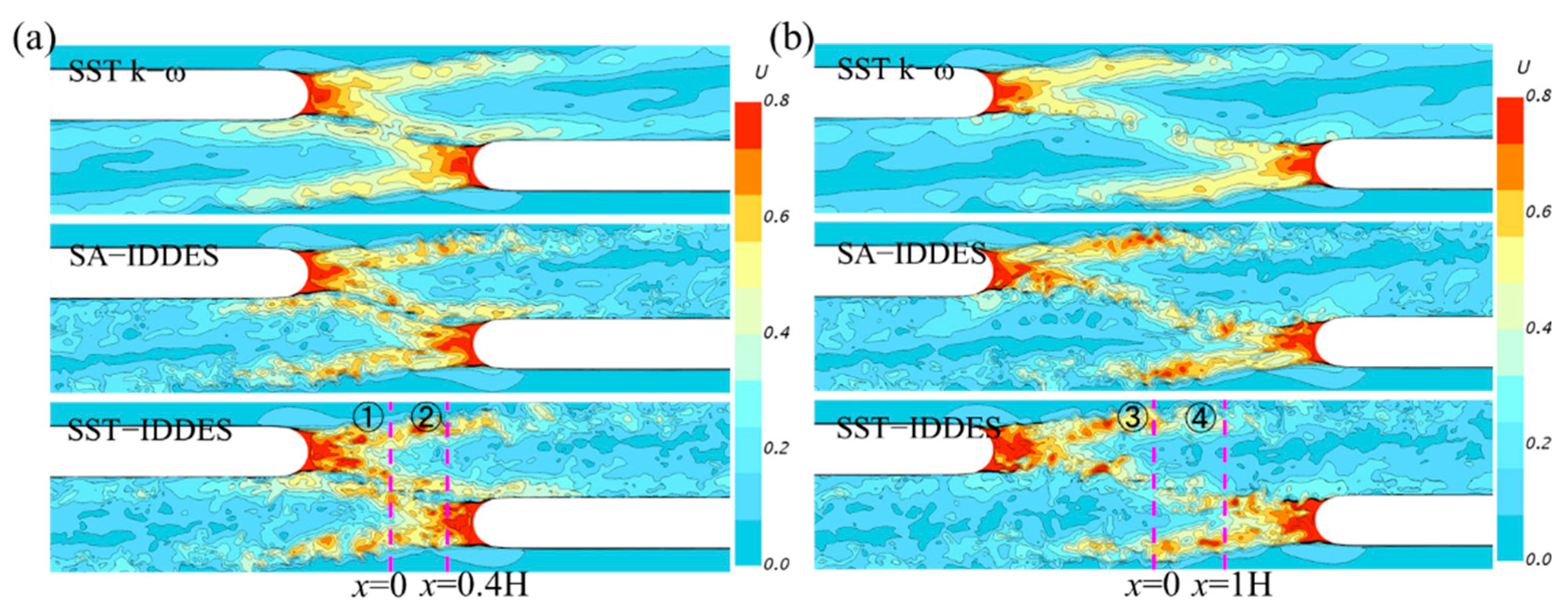
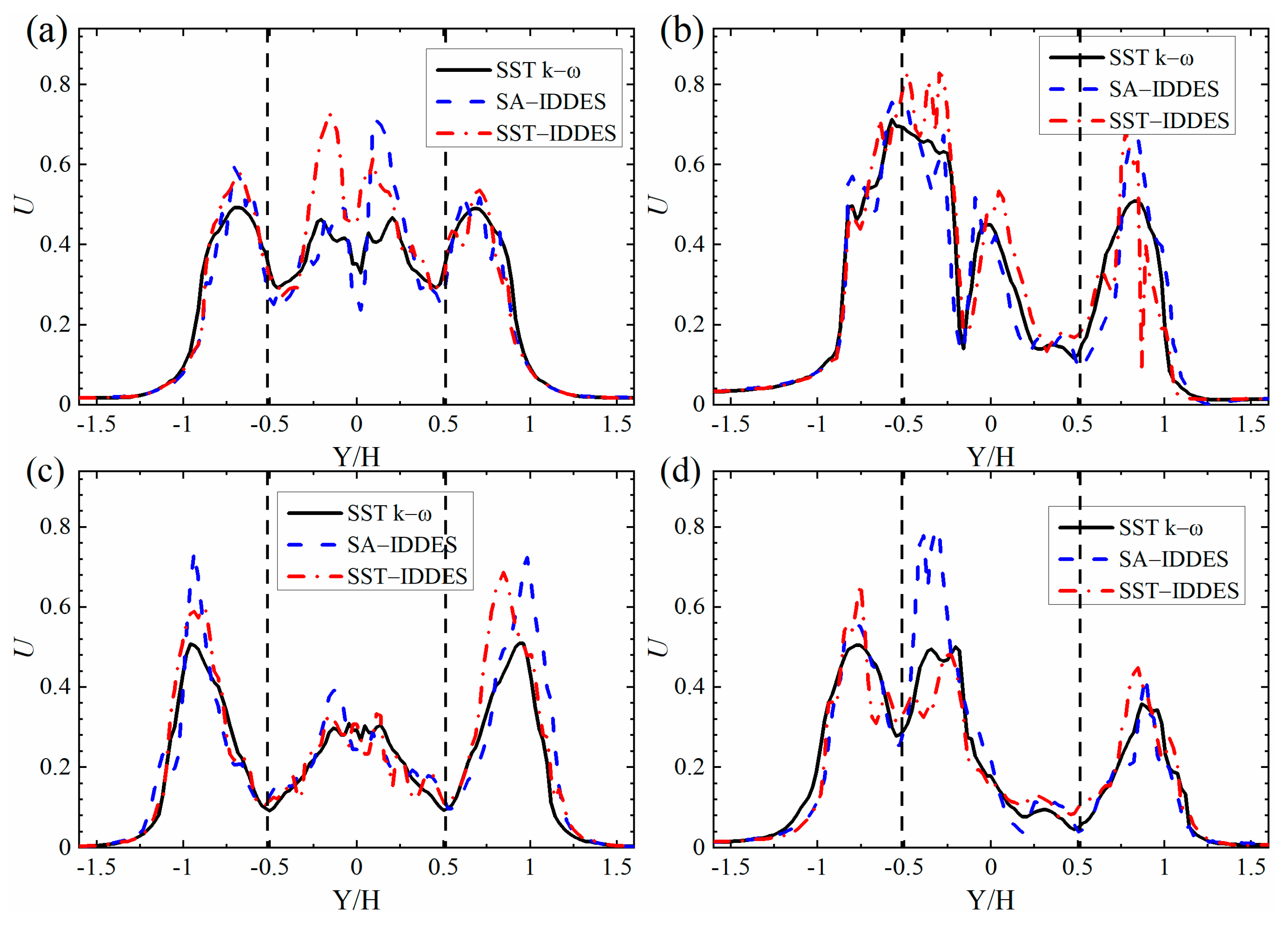
3.2. Velocity Profiles
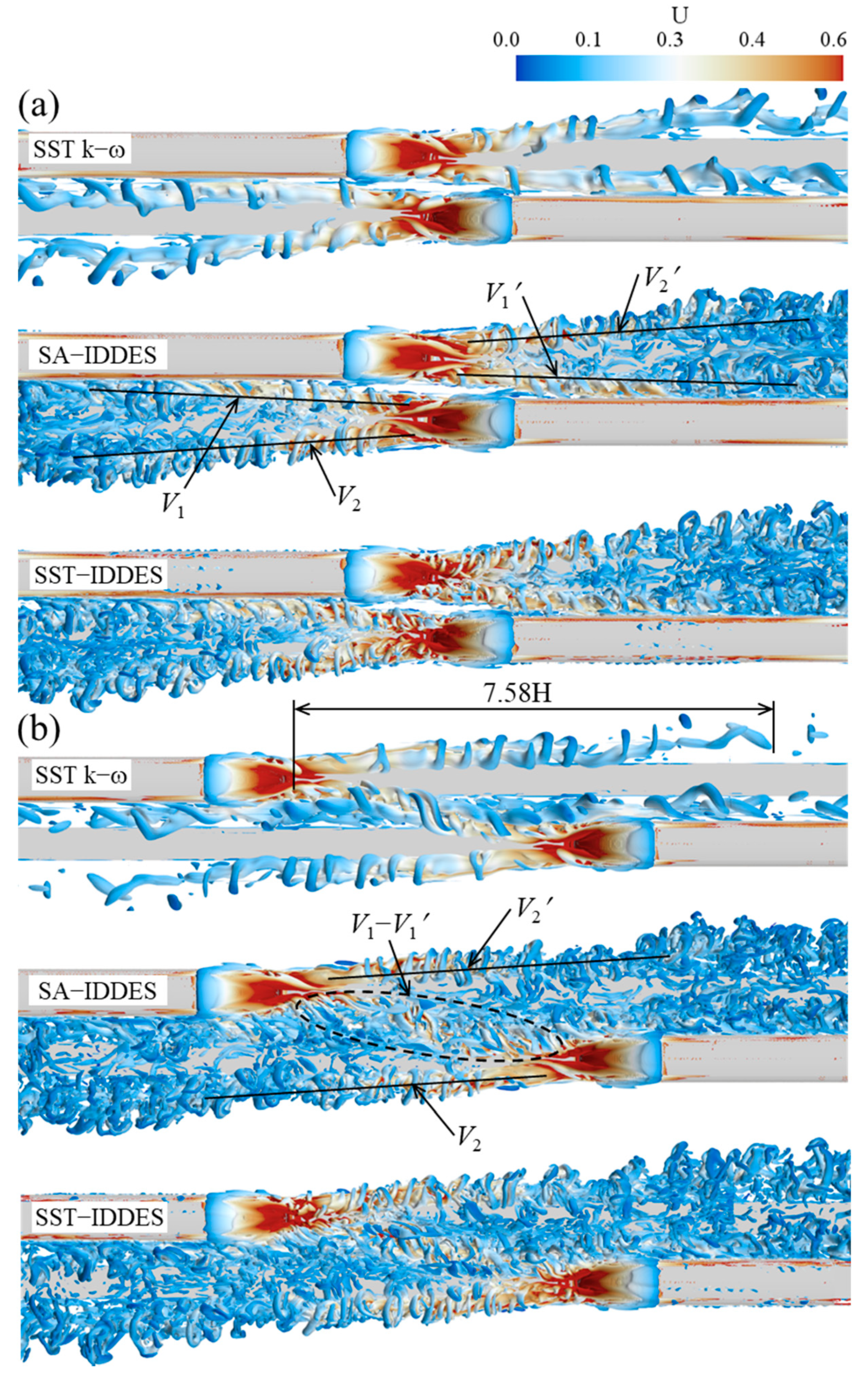
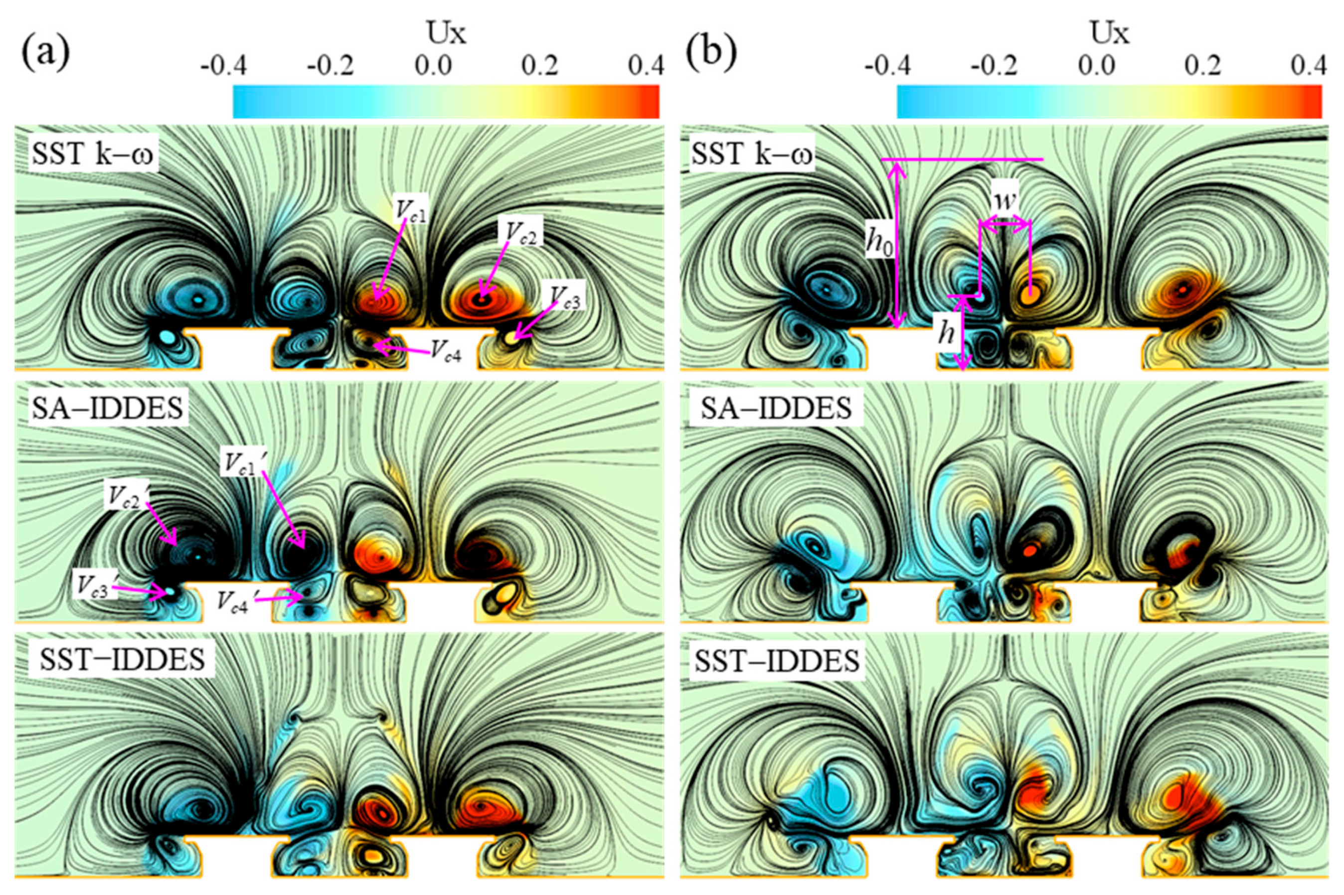
3.3. Wake Flows
3.4. Aerodynamic Forces
4. Conclusions
Author Contributions
Funding
Institutional Review Board Statement
Informed Consent Statement
Data Availability Statement
Conflicts of Interest
References
- Huang, S.; Li, Z.; Yang, M. Aerodynamics of high-speed maglev trains passing each other in open air. J. Wind Eng. Ind. Aerodyn. 2019, 188, 151–160. [Google Scholar] [CrossRef]
- Sun, Z.; Zhang, Y.; Guo, D.; Yang, G.; Liu, Y. Research on Running Stability of CRH3 High Speed Trains Passing by Each Other. Eng. Appl. Comp. Fluid Mech. 2014, 8, 140–157. [Google Scholar] [CrossRef]
- Zhao, Y.; Zhang, J.; Li, T.; Zhang, W. Aerodynamic performances and vehicle dynamic response of high-speed trains passing each other. J. Mod. Transp. 2012, 20, 36–43. [Google Scholar] [CrossRef][Green Version]
- MacNeill, R.A.; Holmes, S.; Lee, H.S. Measurement of the aerodynamic pressures produced by passing trains. In Proceedings of the ASME/IEEE Joint Railroad Conference, Washington, DC, USA, 23–25 April 2002; pp. 57–64. [Google Scholar]
- Mancini, G.; Malfatti, A. Full Scale Measurements on High Speed Train Etr 500 Passing in Open Air and in Tunnels of Italian High Speed Line; Springer: Berlin/Heidelberg, Germany, 2002; pp. 101–122. [Google Scholar] [CrossRef]
- Hwang, J.; Lee, D.-H. Unsteady aerodynamic loads on high speed trains passing by each other. KSME Int. J. 2000, 14, 867–878. [Google Scholar] [CrossRef]
- Johnson, T.; Dalley, S. 1/25 Scale Moving Model Tests for the TRANSAERO Project; Springer: Berlin/Heidelberg, Germany, 2002; pp. 123–135. [Google Scholar] [CrossRef]
- Raghunathan, R.S.; Kim, H.D.; Setoguchi, T. Aerodynamics of high-speed railway train. Prog. Aeosp. Sci. 2002, 38, 469–514. [Google Scholar] [CrossRef]
- Muñoz-Paniagua, J.; García, J. Aerodynamic surrogate-based optimization of the nose shape of a high-speed train for crosswind and passing-by scenarios. J. Wind Eng. Ind. Aerodyn. 2019, 184, 139–152. [Google Scholar] [CrossRef]
- Wu, H.; Zhou, Z.-j. Study on aerodynamic characteristics and running safety of two high-speed trains passing each other under crosswinds based on computer simulation technologies. J. Vibroeng. 2017, 19, 6328–6345. [Google Scholar] [CrossRef]
- Liu, F.; Yao, S.; Zhang, J.; Zhang, N. Aerodynamic effect of EMU passing by each other under crosswind. J. Cent. South Univ. 2016, 47, 307–313. [Google Scholar]
- Luo, C.; Zhou, D.; Chen, G.; Krajnovic, S.; Sheridan, J. Aerodynamic Effects as a Maglev Train Passes Through a Noise Barrier. Flow Turbul. Combust. 2020, 105, 761–785. [Google Scholar] [CrossRef]
- Yau, J.D. Aerodynamic vibrations of a maglev vehicle running on flexible guideways under oncoming wind actions. J. Sound Vibr. 2010, 329, 1743–1759. [Google Scholar] [CrossRef]
- Yu, R.Z. The Characteristics of Aerodynamic Study on CRH380A High-Speed Train. Master’s Thesis, Southwest Jiaotong University, Chengdu, China, 2014. [Google Scholar]
- Chen, J.X. Study on Crossing air Pressure Pulse and Aerodynamic Performance of High-Speed Maglev Trains Meeting in the Open Air. Master’s Thesis, Lanzhou Jiaotong University, Lanzhou, China, 2018. [Google Scholar]
- Zhou, D.; Tian, H.Q.; Lu, Z.J. Optimization of aerodynamic shape for domestic maglev vehicle. J. Cent. South Univ. 2006, 37, 613–617. [Google Scholar]
- Bell, J.R.; Burton, D.; Thompson, M.; Herbst, A.; Sheridan, J. Wind tunnel analysis of the slipstream and wake of a high-speed train. J. Wind Eng. Ind. Aerodyn. 2014, 134, 122–138. [Google Scholar] [CrossRef]
- Li, X.; Chen, G.; Zhou, D.; Chen, Z. Impact of Different Nose Lengths on Flow-Field Structure around a High-Speed Train. Appl. Sci. 2019, 9, 4573. [Google Scholar] [CrossRef]
- Wang, S.; Burton, D.; Herbst, A.; Sheridan, J.; Thompson, M.C. The effect of bogies on high-speed train slipstream and wake. J. Fluids Struct. 2018, 83, 471–489. [Google Scholar] [CrossRef]
- Heinz, S. A review of hybrid RANS-LES methods for turbulent flows: Concepts and applications. Prog. Aeosp. Sci. 2020, 114, 100597. [Google Scholar] [CrossRef]
- Liang, X.-F.; Chen, G.; Li, X.-B.; Zhou, D. Numerical simulation of pressure transients caused by high-speed train passage through a railway station. Build. Environ. 2020, 184, 107228. [Google Scholar] [CrossRef]
- Tan, C.; Zhou, D.; Chen, G.; Sheridan, J.; Krajnovic, S. Influences of marshalling length on the flow structure of a maglev train. Int. J. Heat Fluid Flow 2020, 85, 108604. [Google Scholar] [CrossRef]
- Li, X.; Chen, G.; Krajnovic, S.; Zhou, D. Numerical Study of the Aerodynamic Performance of a Train with a Crosswind for Different Embankment Heights. Flow Turbul. Combust. 2021, 107, 105–123. [Google Scholar] [CrossRef]
- CEN European Standard. Part 4: Requirements and Test Procedures for Aerodynamics on Open Track. In Railway Applications-Aerodynamics; CEN EN 14067-4; BSI Standards Limited: London, UK, 2013; Available online: https://infostore.saiglobal.com/preview/is/en/2013/i.s.en14067-4-2013.pdf?sku=1694040 (accessed on 5 October 2021).
- Niu, J.Q.; Zhou, D.; Liu, T.H.; Liang, X.F. Numerical simulation of aerodynamic performance of a couple multiple units high-speed train. Veh. Syst. Dyn. 2017, 55, 681–703. [Google Scholar] [CrossRef]
- Hemida, H.; Krajnović, S. LES study of the influence of the nose shape and yaw angles on flow structures around trains. J. Wind Eng. Ind. Aerodyn. 2010, 98, 34–46. [Google Scholar] [CrossRef]
- Krajnović, S.; Ringqvist, P.; Nakade, K.; Basara, B. Large eddy simulation of the flow around a simplified train moving through a crosswind flow. J. Wind Eng. Ind. Aerodyn. 2012, 110, 86–99. [Google Scholar] [CrossRef]
- Shur, M.L.; Spalart, P.R.; Strelets, M.K.; Travin, A.K. A hybrid RANS-LES approach with delayed-DES and wall-modelled LES capabilities. Int. J. Heat Fluid Flow 2008, 29, 1638–1649. [Google Scholar] [CrossRef]
- Wang, J.; Minelli, G.; Dong, T.; Chen, G.; Krajnović, S. The effect of bogie fairings on the slipstream and wake flow of a high-speed train. An IDDES study. J. Wind Eng. Ind. Aerodyn. 2019, 191, 183–202. [Google Scholar] [CrossRef]
- Luckhurst, S.; Varney, M.; Xia, H.; Passmore, M.A.; Gaylard, A. Computational investigation into the sensitivity of a simplified vehicle wake to small base geometry changes. J. Wind Eng. Ind. Aerodyn. 2019, 185, 1–15. [Google Scholar] [CrossRef]
- Meng, S.; Meng, S.; Wu, F.; Li, X.; Zhou, D. Comparative analysis of the slipstream of different nose lengths on two trains passing each other. J. Wind Eng. Ind. Aerodyn. 2021, 208, 104457. [Google Scholar] [CrossRef]
- Krajnovic, S. Numerical simulation of the flow around an ICE2 train under the influence of a wind gust. In Proceedings of the 2008 International Conference on Railway Engineering—Challenges for Railway Transportation in Information Age, Hong Kong, China, 25–28 March 2008; pp. 1–7. [Google Scholar]
- Cross, D.; Hughes, B.; Ingham, D.; Ma, L. A validated numerical investigation of the effects of high blockage ratio and train and tunnel length upon underground railway aerodynamics. J. Wind Eng. Ind. Aerodyn. 2015, 146, 195–206. [Google Scholar] [CrossRef]
- Zhang, N.; Lu, Z.; Zhou, D. Influence of train speed and blockage ratio on the smoke characteristics in a subway tunnel. Tunn. Undergr. Space Technol. 2018, 74, 33–40. [Google Scholar] [CrossRef]
- Khayrullina, A.; Blocken, B.; Janssen, W.; Straathof, J. CFD simulation of train aerodynamics: Train-induced wind conditions at an underground railroad passenger platform. J. Wind Eng. Ind. Aerodyn. 2015, 139, 100–110. [Google Scholar] [CrossRef]
- Li, W.; Liu, T.; Chen, Z.; Guo, Z.; Huo, X. Comparative study on the unsteady slipstream induced by a single train and two trains passing each other in a tunnel. J. Wind Eng. Ind. Aerodyn. 2020, 198, 104095. [Google Scholar] [CrossRef]
- Niu, J.; Zhou, D.; Liang, X.; Liu, T.; Liu, S. Numerical study on the aerodynamic pressure of a metro train running between two adjacent platforms. Tunn. Undergr. Space Technol. 2017, 65, 187–199. [Google Scholar] [CrossRef]
- Liu, Z.; Chen, G.; Zhou, D.; Wang, Z.; Guo, Z. Numerical investigation of the pressure and friction resistance of a high-speed subway train based on an overset mesh method. Proc. Inst. Mech. Eng. Part F-J. Rail Rapid Transit 2021, 235, 598–615. [Google Scholar] [CrossRef]
- Yao, Z.; Zhang, N.; Chen, X.; Zhang, C.; Xia, H.; Li, X. The effect of moving train on the aerodynamic performances of train-bridge system with a crosswind. Eng. Appl. Comput. Fluid Mech. 2020, 14, 222–235. [Google Scholar] [CrossRef]
- Hunt, J.C.R.; Wray, A.A.; Moin, P. Eddies, streams, and convergence zones in turbulent flows. Stanf. Cent. Turbul. Res. Rep. CTR-S88 1988, 193–208. [Google Scholar]
- Zhang, L.; Yang, M.-Z.; Liang, X.-F.; Zhang, J. Oblique tunnel portal effects on train and tunnel aerodynamics based on moving model tests. J. Wind Eng. Ind. Aerodyn. 2017, 167, 128–139. [Google Scholar] [CrossRef]
- Wang, S.; Bell, J.R.; Burton, D.; Herbst, A.H.; Sheridan, J.; Thompson, M.C. The performance of different turbulence models (URANS, SAS and DES) for predicting high-speed train slipstream. J. Wind Eng. Ind. Aerodyn. 2017, 165, 46–57. [Google Scholar] [CrossRef]
- Li, T.; Hemida, H.; Zhang, J.; Rashidi, M.; Flynn, D. Comparisons of Shear Stress Transport and Detached Eddy Simulations of the Flow around Trains. J. Fluids Eng.-Trans. ASME 2018, 140, 111108. [Google Scholar] [CrossRef]


| Grid | Coarse | Medium | Fine |
|---|---|---|---|
| Train surface | 0.016 H | 0.013 H | 0.01 H |
| Wake refinement | 0.016 H | 0.013 H | 0.01 H |
| Number of prism layers | 16 | 20 | 20 |
| Number of cells (×106) | 27.17 | 45.75 | 68.39 |
Publisher’s Note: MDPI stays neutral with regard to jurisdictional claims in published maps and institutional affiliations. |
© 2021 by the authors. Licensee MDPI, Basel, Switzerland. This article is an open access article distributed under the terms and conditions of the Creative Commons Attribution (CC BY) license (https://creativecommons.org/licenses/by/4.0/).
Share and Cite
Li, X.; Krajnovic, S.; Zhou, D. Numerical Study of the Unsteady Aerodynamic Performance of Two Maglev Trains Passing Each Other in Open Air Using Different Turbulence Models. Appl. Sci. 2021, 11, 11894. https://doi.org/10.3390/app112411894
Li X, Krajnovic S, Zhou D. Numerical Study of the Unsteady Aerodynamic Performance of Two Maglev Trains Passing Each Other in Open Air Using Different Turbulence Models. Applied Sciences. 2021; 11(24):11894. https://doi.org/10.3390/app112411894
Chicago/Turabian StyleLi, Xianli, Siniša Krajnovic, and Dan Zhou. 2021. "Numerical Study of the Unsteady Aerodynamic Performance of Two Maglev Trains Passing Each Other in Open Air Using Different Turbulence Models" Applied Sciences 11, no. 24: 11894. https://doi.org/10.3390/app112411894
APA StyleLi, X., Krajnovic, S., & Zhou, D. (2021). Numerical Study of the Unsteady Aerodynamic Performance of Two Maglev Trains Passing Each Other in Open Air Using Different Turbulence Models. Applied Sciences, 11(24), 11894. https://doi.org/10.3390/app112411894