Simulation of the Marangoni Effect and Phase Change Using the Particle Finite Element Method

Abstract

A simulation method is developed herein based on the particle finite element method (PFEM) to simulate processes with surface tension and phase change. These effects are important in the simulation of industrial applications, such as welding and additive manufacturing, where concentrated heat sources melt a portion of the material in a localized fashion. The aim of the study is to use this method to simulate such processes at the meso-scale and thereby gain a better understanding of the physics involved. The advantage of PFEM lies in its Lagrangian description, allowing for automatic tracking of interfaces and free boundaries, as well as its robustness and flexibility in dealing with multiphysics problems. A series of test cases is presented to validate the simulation method for these two effects in combination with temperature-driven convective flows in 2D. The PFEM-based method is shown to handle both purely convective flows and those with the Marangoni effect or melting well. Following exhaustive validation using solutions reported in the literature, the obtained results show that an overall satisfactory simulation of the complex physics is achieved. Further steps to improve the results and move towards the simulation of actual welding and additive manufacturing examples are pointed out.

1. Introduction

Phase change plays a key role in some state-of-the-art manufacturing processes, such as welding and additive manufacturing. Characteristic of these applications is that phase change occurs very locally at a specific length scale, which we call the mesoscale. The mesoscale is the length scale at which the melt pool and the concentrated heat source are well-resolved. Other phenomena relevant to engineers occur on all length scales while still strongly depending on phenomena at the mesoscale. Examples include residual stresses and material warping at the part scale and the crystallographic evolution upon freezing at the microscale, which are closely related to convective flows, heat transfer and melt pool evolution at the mesoscale. Few methods have been developed that can fully or even partially simulate these effects at the mesoscale.

In the literature, there are some examples of simulation methods that neglect the fluid flow altogether and only concentrate on solid mechanics and heat transfer at the mesoscale. Some authors [1,2,3] use a Eulerian or Lagrangian finite element method (FEM) to obtain the temperature field around the laser heat source in selective laser melting (SLM). The latter includes elasto-perfectly plastic behavior of the liquid melt pool; however, no convective flows are modeled that would greatly influence the heat transfer. The focus lies more on the accurate representation of the solid behavior under strong temperature gradients and fast cooling.

Conversely, much work can be found investigating the fluid flow in the melt pool and the evolution of the melt pool geometry. Several authors [4,5] use an Arbitrary Lagrangian–Eulerian (ALE) description of the liquid melt pool, with the former example assuming the powder to be a continuum, and the latter using the discrete element method (DEM) to create a powder bed where individual particles are resolved. The aim of such studies is to explore the physics of the melt pool, such as the recoil pressure from evaporation and the Marangoni effect, as well as other phenomena such as denudation of the powder bed, spattering, pore formation and keyhole evolution.

The most common approach for simulating melt pool fluid dynamics is the use of the finite volume method (FVM) in combination with an interface tracking method such as Level set (LS) or Volume of Fluid (VoF). Often, the powder bed is created using the DEM. This is done by many groups, and a good summary can be found in Cook and Murphy’s review paper [6]. The modelling of the solid mechanics is omitted in all of these works, which are thus geared towards predicting melt track topology and provide impressive results thereof.

There are limited examples of other methods used for welding and additive manufacturing, such as smoothed particle hydrodynamics (SPH) and the lattice Boltzmann method (LBM). Both share the drawback that some boundary conditions and the Marangoni effect are difficult to implement, making these a rare choice in the context of additive manufacturing. See also Cook and Murphy [6] for details.

One particularly noteworthy work devoted to the modeling of the additive manufacturing process in which the problem is split into a solid and fluid parts is that of Chen [7]. The powder is modeled as a flowable continuum, and hence included in the fluid part. For the fluid phase, a Eulerian FEM code for Newtonian fluids with a level set method for interface tracking together with remeshing at regular intervals is used. For the solid, a separate Eulerian FEM code with an elasto-plastic solid model is used. Both are coupled and solved in sequence for each time increment. While the fluid and powder are solved using the Navier–Stokes equations, the solid region in the domain is also included, although with an extremely high viscosity. Based on the fluid flow and the heat transfer, the melt pool can evolve in this step. Then, only the new outlines of the melt pool and the temperature profile are transferred to the solid solver. There, the yield stress reduces to zero in the fluid and powder regions. This means that the fluids can deform without any resistance, while the actual solid around the melt pool deforms elasto-plastically. To our best knowledge, this is the only approach that incorporates both the convective flow in the melt pool (to obtain a realistic heat transfer) and the elasto-plastic solid (to obtain residual stresses) in one single simulation method. Chen obtains excellent agreement with experimental results. The main drawbacks of this method are the complex and expensive coupling and the necessity of using the level set interface tracking, which further increases cost and complexity.

As an alternative approach we use the Particle Finite Element Method (PFEM), which can be described as a Lagrangian FEM with frequent and automatic remeshing to avoid mesh distortions, even when simulating fluid flow [8]. The Lagrangian description allows the free surface to deform without the need for an interface tracking technique. The remeshing algorithm also includes the alpha shape technique [9], which makes the remeshing fully automatic even when large or chaotic deformations of the free surface occur (e.g., sloshing, breaking waves, splashing etc.). The main advantage of the PFEM is its proven capability to simulate fluids [10], thermo-fluids [11,12], solids [13] and thermo-solids [14,15,16]. A further advantage is its robustness, as it is based on the mature FEM. It has also been shown that free surface deformation and surface tension can easily be included in the PFEM [17]. Many works focus on fluid–structure interaction (FSI) using the PFEM [18,19,20,21], and one work that we are aware of includes phase change, in which Franci et al. [22] simulate a core melt accident in a nuclear power station using the PFEM. Other than this, PFEM has not been utilized for phase change problems, despite its unique capability to simulate fluids and solids equally well. An extensive yet concise review on PFEM was recently published by Cremonesi et al. [17], where more details are explained and the different directions of recent research into PFEM are outlined.

In this work, we aim to show the general suitability of PFEM in the context of additive manufacturing and welding at the mesoscale. The focus lies on the evolution of the melt pool and the physics that drive fluid flow, such as buoyancy and the Marangoni effect. Two main simplifications are made at this stage of our in-house PFEM code development. First, the solid material is replaced by a fluid with a momentum sink term that prevents further deformation upon freezing, instead of using an elasto-plastic solid. Secondly, all simulations use the 2D plain strain assumption. These simplifications are planned to be abandoned in the future to arrive at a simulation method that can simulate both phase change, convective flows in the melt pool and residual stresses in the solid in 3D. To demonstrate the suitability of the method for simulations with phase change and fluid dynamics, three validation test cases are presented and compared against the results from the literature. Known limitations of PFEM include the increased computational cost due to the frequent remeshing when compared with traditional FEM. Furthermore, with the connectivity changing constantly, parallelization of the solving process is difficult and is not included in the present code. Other than that, the limitations are those of traditional FEM.

The novelty of this work lies in the utilization of PFEM for phase change, which has only been published once before and that with limited focus on the intricacies of latent heat and the transition from solid to fluid. Applications such as welding and additive manufacturing are characteristically sensitive to accurate representation of the phase transition. This work serves as validation for the simulation of welding and additive manufacturing applications in the future.

2. Governing Equations and Solution Methods

2.1. Kinematic Description

Using the Lagrangian description, the frame of reference follows the material as it moves and deforms. This facilitates keeping track of the history of a material particle, (which is necessary for certain constitutive models, e.g., elasto-plastic materials) as well as keeping track of deforming boundaries and interfaces. As the bulk of a material deforms, its boundaries deform with it, eliminating the necessity of dedicated boundary and interface tracking methods. This is a substantial advantage over more traditional Eulerian methods. The notable disadvantage of the Lagrangian description is the deformation and subsequent distortion of the mesh, which is avoided through continuous re-meshing.

2.2. Navier–Stokes Equations

The Navier–Stokes equations include the linear momentum conservation equation and the continuity equation. The continuity equation for incompressible media can be written in its local form as

$$\nabla \cdot \mathit{v}=0,$$

(1)

where $\nabla \cdot \left( \right)$ is the divergence operator and $v$ is the velocity vector. The conservation of linear momentum is written in the Lagrangian form as

$$\rho \frac{dv}{dt}-\nabla \cdot \mathit{\sigma }-\rho \mathit{b}-\mathit{s}=0,$$

(2)

where $\rho$ is the density, $d/dt\left( \right)$ is the material time derivative, $\mathit{\sigma }$ is the Cauchy stress tensor and $\mathit{b}$ is the body force vector, which usually represents gravitational acceleration in $y$-direction $g=-9.81 \mathrm{m}/{\mathrm{s}}^2$ unless otherwise stated. $\mathit{s}$ is a source term that permits adding or removing momentum, which we utilized for the solid phase as explained in Section 2.5 For the momentum equation, the Dirichlet and Neumann boundary conditions are

$$\mathit{v}\left(\mathit{x},t\right)=\overline{\mathit{v}}\left(\mathit{x},t\right) {\mathrm{on} \mathsf{\Gamma }}_{\mathrm{v}}$$

(3)

$$\mathit{\sigma }\left(\mathit{x},t\right)\cdot \mathit{n}=\overline{\mathit{t}}\left(\mathit{x},t\right) {\mathrm{on} \mathsf{\Gamma }}_{\mathrm{t}}$$

(4)

where $\mathit{x}$ is the current location in space, $\overline{\mathit{v}}$ is the imposed velocity and $\overline{\mathit{t}}$ is the imposed surface traction. ${\mathsf{\Gamma }}_v$ and ${\mathsf{\Gamma }}_t$ are the parts of the boundary $\mathsf{\Gamma }$ where velocity or traction is imposed, respectively, such that ${\mathsf{\Gamma }}_v\cup {\mathsf{\Gamma }}_t=\mathsf{\Gamma }$ and ${\mathsf{\Gamma }}_v\cap {\mathsf{\Gamma }}_t=\varnothing$. Next, a Newtonian fluid constitutive law is introduced,

$$\mathit{\sigma }=-p\mathbf{I}+2\mu \dot{\mathit{\epsilon }},$$

(5)

where $p$ is the pressure, $\mathbf{I}$ is the identity matrix, $\mu$ is the dynamic viscosity and $\dot{\mathit{\epsilon }}$ is the strain rate, which can be re-written in terms of velocity $\mathit{v}$ as

$$\mathit{\sigma }=-p\mathbf{I}+\mu \left(\nabla \mathit{v}+\nabla {\mathit{v}}^T\right).$$

(6)

Injecting the constitutive law (6) into the momentum Equation (2) and re-writing in the Lagrangian form gives us the strong form of the incompressible Navier–Stokes momentum equation:

$$\rho \frac{d\mathit{v}}{dt}+\nabla p-\mu \nabla \cdot \left(\nabla \mathit{v}+\nabla {\mathit{v}}^T\right)-\rho \mathit{b}-\mathit{s}=0.$$

(7)

2.3. Traction Term at the Free Surface

At the free surface, external forces such as the atmospheric pressure and surface tension forces are applied through the surface traction vector $\overline{t}$, which is be split into its tangential and normal components:

$$\overline{\mathit{t}}=t_n\mathit{n}+t_t\mathit{t},$$

(8)

where in 2D $t_n$ and $t_t$ are the magnitudes of normal and in-plane tangential surface traction and $n$ and $t$ are the normal and tangent vectors on the boundary ${\mathsf{\Gamma }}_t$. In this work, only test cases with a Eulerian description were replicated for the purpose of validation. Hence, the free surface is not able to deform in the normal direction and we therefore have

$$t_n=0.$$

(9)

The Marangoni effect is a tangential force caused by a gradient in surface tension which itself is caused by a gradient in temperature. In the case of welding or additive manufacturing, the concentrated heat source on the liquid melt pool creates a large gradient of temperature along the surface, leading to the Marangoni effect, which is found to be a main driving force for convective flows in the melt pool [23,24]. The Marangoni shear stress $t_t$ can be modeled using the equation

$$t_t=\frac{\partial \gamma }{\partial T}{\nabla }_{t}T=\frac{\partial \gamma }{\partial T}\left(\nabla T-\left(\mathit{n}\cdot \nabla T\right)\mathit{n}\right),$$

(10)

where ${\nabla }_t$ is the tangential component of the spatial derivative that can be recovered by subtracting the normal component of the temperature gradient from the temperature gradient, as shown on the rightmost part of Equation (10). $\partial \gamma /\partial T$ is a material property that is referred to as the Marangoni coefficient, and can be a function of temperature.

2.4. Buoyancy

The media considered here are incompressible, with the exception of thermal expansion. The density $\rho$ is calculated using

$$\rho ={\rho }_{ref}\exp \left(-{\int }_{T_{ref}}^T{\beta }_V\left(T\right)dT\right)$$

(11)

where ${\rho }_{ref}$ is the reference density at a reference temperature $T_{ref}$ and ${\beta }_V$ is the coefficient of volumetric thermal expansion. The effect of thermal expansion on the continuity equation (local volume change) is neglected. Only the change in density in the body force term in Equation (7) is taken into account, recovering the well-known Boussinesq approximation.

2.5. Phase Change and Solid Flow Resistance

To model the changes in the momentum equation for the two phases, we must first define the phase fraction $f_p$ that indicates the resulting phase as a function of temperature, where $f_p=1$ marks a liquid, $f_p=0$ marks a solid and $0<f_p<1$ marks the mushy zone. We use the following definition for $f_p$:

$$f_p=\left\{\begin{array}{ccc}1& \mathrm{for} T\ge T_l\hfill & \\ \frac{T-T_s}{T_l-T_s}& \mathrm{for} T_l>T>T_l\hfill & \\ 0& \mathrm{for} T\le T_s\hfill & ,\end{array}\right.$$

(12)

where $T_l$ and $T_s$ are the liquidus and solidus temperatures that form the phase change interval with a linear distribution inside this interval. Note that more realistic transitions are possible (see for example [25]). In the case of isothermal phase change, both temperatures are equal and there is only the melting temperature, $T_m$. There, the transition of the liquid fraction in Equation (12) collapses into a step function. In the context of numerical methods, such discontinuities can cause instabilities; however, none were observed here and no special treatment was necessary (compare Section 2.7).

When using the Navier–Stokes equations, the treatment of the solid and semi-solid or mushy phases is not straightforward. Instead of changing the constitutive equation for the non-fluid phases, we continue to use the Newtonian fluid law, but add the sink term s to the momentum equation. The purpose of this sink term is to remove momentum locally wherever the material is not fully in the liquid phase. This effectively adds a resistance to the flow as the material freezes. When fully frozen, the sink term removes all momentum and a particle remains fixed. This is a modelling approach that is widely used in the context of phase change simulations with fluid solvers at this length scale [6]. In the literature, the choice of model for the sink term s is often the well-known Carman–Kozeny equation (e.g., [26,27,28]):

$$\mathit{s}=-C\frac{{\left(1-f_p\right)}^2}{\epsilon +f_p^3}\mathit{v}$$

(13)

where $C$ is the drag coefficient, which must be large, and $\epsilon$ is a small coefficient that is used to avoid division by zero. This equation is normally used to describe the pressure drop of a flow through a porous medium, which may not accurately represent the mushy zone in a welding or additive manufacturing application. However, it appears that the equation is widely used because it is a reasonable approximation of the physics without being prohibitively complicated. According to Cook and Murphy [6], the parameters are usually arbitrarily chosen to be on the order of $C={10}^5{ \mathrm{kg} \mathrm{m}}^{-3} {\mathrm{s}}^{-1}$ and $\epsilon ={10}^{-5}$, although different sources use different values without explaining their specific choice.

To summarize, this term subtracts momentum from a particle as it approaches the solid state. When fully solid (i.e., $f_p=0$), the velocity is nearly zero. Conversely, when fully liquid (i.e., $f_p=1$), this entire term becomes zero and the regular Navier–Stokes equations are recovered.

2.6. Heat Equation

The heat equation is used in the form of the so-called temperature equation,

$$\rho c_p\frac{dT}{dt}+\nabla \cdot \mathit{q}-Q-L=0,$$

(14)

where $c_p$ is the specific isobaric heat capacity, $T$ is the temperature, $\mathit{q}$ is the heat flux vector, $Q$ is the external volumetric heat source term and $L$ is the latent heat term. The boundary conditions are

$$T\left(\mathit{x},t\right)=\overline{T}\left(\mathit{x},t\right) \mathrm{on} {\mathsf{\Gamma }}_T$$

(15)

$$\mathit{q}\left(\mathit{x},t\right)\cdot n=\overline{q}\left(\mathit{x},t\right) {\mathrm{on} \mathsf{\Gamma }}_q,$$

(16)

where $\overline{T}$ is the imposed temperature, $\overline{q}$ is the imposed surface heat flux, and ${\mathsf{\Gamma }}_T$ and ${\mathsf{\Gamma }}_q$ are the parts of the boundary $\mathsf{\Gamma }$ such that ${\mathsf{\Gamma }}_T\cup {\mathsf{\Gamma }}_q=\mathsf{\Gamma }$ and ${\mathsf{\Gamma }}_T\cap {\mathsf{\Gamma }}_q=\varnothing$. The constitutive law for the heat equation is Fourier’s law, which reads

$$\mathit{q}=-\kappa \nabla T$$

(17)

where $\kappa$ is the conductivity of an isotropic material. Inserting Equation (17) into Equation (14) gives us the final form of the temperature equation,

$$\rho c_p\frac{dT}{dt}-\nabla \cdot \left(\mathit{\kappa }\nabla T\right)-Q-L=0$$

(18)

Note that in this work, when replicating test cases from the literature no heat source or imposed surface heat flux appears except for adiabatic boundaries, where $\overline{q}=0$ on ${\mathsf{\Gamma }}_q$.

2.7. Latent Heat Term

The latent heat of fusion that is absorbed or released upon melting and freezing, respectively, is non-linear and spatially very localized, with a high magnitude. In the context of numerical simulation, this can cause oscillations and convergence issues. In our work, the latent heat is treated as a separate source term, although some authors incorporate it into the heat capacity term. The specific enthalpy h stored in the material at any point is

$$h=\mathsf{\Delta }{h}_L{f}_p\left(T\right)+{\int }_0^T\rho c_p\left(T\right)$$

(19)

where $\mathsf{\Delta }{h}_L$ is the latent heat of fusion (a material property) and $f_p$ is the phase fraction, defined in Equation (12). The first term is the latent heat and the second term is the sensible heat of the material for any given temperature $T$. The rate at which the latent heat is stored or released is thus

$$L=\frac{d}{dt}\left(\mathsf{\Delta }{h}_L{f}_p\right)=\mathsf{\Delta }{h}_L\frac{d{f}_p}{dT}\frac{dT}{dt}.$$

(20)

In the worst case, with isothermal phase change the phase fraction function $f_p\left(T\right)$ becomes a step function at the melting point $T_m$, and the derivative with respect to temperature hence becomes infinite. Even when $f_p\left(T\right)$ is not a step but rather a steep ramp, numerical problems can arise and regularization is needed, as in Figure 1a.

A regularization is a smoothing of the discontinuous function to restore at least C¹ continuity by replacing the discontinuous function $f_p$ by a function $\widehat{f_p}$ that closely approximates the original but is also sufficiently smooth. We used a cubic function that is tangential at both ends of the regularized interval. In the case of non-isothermal phase change with a simple ramp function for $f_p$, one can choose to either replace the entire ramp by one cubic function or to replace each side the ramp by an individual cubic function (Figure 1b). The second option was selected here, both for its flexibility and to preserve as much of the original function as possible.

It is worth noting that when $\widehat{f_l}$ is not a good approximation for $f_l$, the non-linear algorithm may not be able to approximate the physically correct solution very well and may prevent the iterative solution from converging, depending on how badly chosen the regularization is. Assuming that a cubic function is used for $\widehat{f_l}$, there is one freely chosen parameter, and it is this that determines the width, ∆T_reg, of the interval. It has been found that with a good spatial resolution and the Newton–Raphson non-linear iterations for the heat equation, a very small ∆T_reg works very well and no oscillations are encountered.

2.8. Weak Form, Discretization and Integration

The PFEM was chosen as the underlying method due to its favorable properties, as briefly outlined in the introduction. Being based on the well-known finite element method (FEM), Equations (1), (7) and (18) are written in the weak form to reduce the differentiability requirements. We define

$$\mathit{v}\in \mathcal{S}, \mathcal{S}=\{\mathit{v}\in H^1\left(\mathsf{\Omega }\right) | \mathit{v}=\overline{\mathit{v}}{ \mathrm{on} \mathsf{\Gamma }}_{\mathrm{v}}\}$$

(21)

$$\mathit{w}\in {\mathcal{S}}_0, {\mathcal{S}}_0=\{\mathit{w}\in H^1\left(\mathsf{\Omega }\right) | \mathit{w}=\mathbf{0} {\mathrm{on} \mathsf{\Gamma }}_{\mathrm{v}}\}$$

(22)

$$p\in \mathcal{Q}, \mathcal{Q}=\left\{q\in L^2\left(\mathsf{\Omega }\right)\right\}$$

(23)

$$T\in \mathcal{R}, \mathcal{R}=\left\{r\in L^2\left(\mathsf{\Omega }\right)\right\}$$

(24)

where $\mathcal{S}$ is the space of vector trial functions for the velocity, ${\mathcal{S}}_0$ is the space of vector test functions for the velocity, $\mathcal{Q}$ is the space of scalar test functions for the pressure and $\mathcal{R}$ is the space of scalar test function for the temperature. $H^1\left(\mathsf{\Omega }\right)$ denotes the space of square integrable functions with square integrable first derivative and $L^2\left(\mathsf{\Omega }\right)$ denotes the space of square integrable functions over the domain $\mathsf{\Omega }$. By multiplying the equations by a smooth and kinematically admissible scalar test function $q$ or a vector test function $\mathit{w}$, taking the integral over the volume, and then integrating by parts, the weak form is obtained. The weak forms of Equations (1), (7) and (18), respectively, are:

$${\int }_{\mathsf{\Omega }}q\nabla \cdot v dV=0 \forall q\in \mathcal{Q}$$

(25)

$$\begin{array}{c}{\int }_{\mathsf{\Omega }}\left(\rho \frac{dv}{dt}\cdot \mathit{w} +p\nabla \cdot \mathit{w}-\mu \left(\nabla \mathit{v} :\nabla \mathit{w}+\nabla {\mathit{v}}^T : \nabla \mathit{w}\right)-\rho \mathit{b}\cdot \mathit{w}-\mathit{s}\cdot \mathit{w}\right)dV\\ +{\int }_{{\mathsf{\Gamma }}_t}\overline{\mathit{t}}\cdot \mathit{w} dS=0 \forall \mathit{w}\in {\mathcal{S}}_0\end{array}$$

(26)

$${\int }_{\mathsf{\Omega }}\left(r\rho c_p\frac{dT}{dt}-r\nabla \cdot \left(\kappa \nabla T\right)-rQ-rL\right)dV+{\int }_{{\mathsf{\Gamma }}_t}r\overline{q} dS=0 \forall r\in \mathcal{R}$$

(27)

and solve for $v\in \mathcal{S}\times \left[t_0, t_{end}\right]$, $p\in \mathcal{Q}\times \left[t_0,t_{end}\right]$ and $T\in \mathcal{R}\times \left[t_0,t_{end}\right].$ To solve the equations using discrete elements, the continuous solution variables of velocity $\mathit{v}\left(\mathit{x},t\right)$, pressure $p\left(\mathit{x},t\right)$ and temperature $T\left(\mathit{x},t\right)$ are discretized. This can be achieved with the Galerkin method, where we use the approximations

$$p\left(\mathit{x},t\right)\approx N_s^T\left(\mathit{x}\right) p\left(t\right)$$

(28)

$$\mathit{v}\left(\mathit{x},t\right)\approx N_v^T\left(\mathit{x}\right) v\left(t\right)$$

(29)

$$T\left(\mathit{x},t\right)\approx N_s^T\left(\mathit{x}\right) T\left(t\right)$$

(30)

where $p$ is the vector of nodal pressures, $v$ is the vector of nodal velocities, $T$ is the vector of nodal temperatures and $N_s$ and $N_v$ are the vectors of linear shape functions. $N_s$ is used for scalar fields and its length equals the number of nodes $n_{nodes}$, whereas $N_v$ is used for vector fields and its length is the $n_{nodes}\cdot n_{dim}$, where $n_{dim}$ is the number of dimensions (here, $n_{dim}=2$).

Using an equal order shape function for both pressure and velocity interpolation is known to violate the Ladyzhenskaya–Babuška–Brezzi (LBB) condition, which allows more than one solution for the pressure field. This leads to undesirable oscillations if left untreated. In this work, the so-called Pressure-Stabilizing Petrov–Galerkin (PSPG) method was chosen to stabilize the solution, as developed by Tezduyar [29]. There, the continuity equation is modified to become

$$-{\int }_{\mathsf{\Omega }}q\nabla \cdot \mathit{v} dV+\tau {\int }_{\mathsf{\Omega }}\frac{1}{\rho }q\left(\rho \frac{d\mathit{v}}{dt} +p\nabla -\rho \mathit{b}-s \right)dV=0$$

(31)

where $\tau$ is a user-chosen parameter. Note that the first term is the original continuity Equation (25); the second term has been added to stabilize the pressure. There, one will recognize that most terms of the momentum Equation (7) re-appear inside the round brackets, which should cancel out, when the momentum equation is converged. The viscous term is missing, as it would require a second derivative in space, which cannot be obtained using linear shape functions. This method is discussed in more detail by Cerquaglia and colleagues in [30].

The discretization in time was done by advancing in time by discrete time steps of length ∆t. The time derivatives acceleration dv/dt and rate of temperature change dT/dt are calculated from velocity v and temperature T, respectively, using the fully implicit backward Euler scheme

$$\frac{d{\varphi }^t}{dt}\approx \frac{{\varphi }^t-{\varphi }^{t-\mathsf{\Delta }t}}{\mathsf{\Delta }t}$$

(32)

where $\varphi$ is a placeholder for $\mathit{v}$ or $T$. The superscripts $t$ and $t-\mathsf{\Delta }t$ refer to the current and previous time steps, respectively. The backward Euler scheme is also used to determine the displacement $\mathit{u}$ of the nodes from $\mathit{v}$:

$${\mathit{x}}^t={\mathit{x}}^{t-\mathsf{\Delta }t}+{\mathit{u}}^t={\mathit{x}}^{t-\mathsf{\Delta }t}+{\mathit{v}}^t\mathsf{\Delta }t.$$

(33)

Inserting Equation (32) into Equations (25)–(27) we get the discretized global system, comprised of the following equations for continuity, momentum and heat:

$$\left(\frac{1}{\mathsf{\Delta }t}C-D\right)\cdot v^t+L_{\tau }\cdot p^t=h+\frac{1}{\mathsf{\Delta }t}C\cdot v^{t-\mathsf{\Delta }t}$$

(34)

$$\left(\frac{1}{\mathsf{\Delta }t}M+K\right)\cdot v^t+D^T\cdot p^t=f+\frac{1}{\mathsf{\Delta }t}M\cdot v^{t-\mathsf{\Delta }t}$$

(35)

$$\left(\frac{1}{\mathsf{\Delta }t}{M}_{th}+K_{th}\right)\cdot T^t=q_{th}+\frac{1}{\mathsf{\Delta }t}{M}_{th}\cdot T^{t-\mathsf{\Delta }t}$$

(36)

where $C$ is the dynamic matrix of the stabilization, $D$ is the discrete divergence operator,$L_{\tau }$ is the pressure Laplacian operator of the stabilization,$h$ is the stabilization term arising from external and body forces, $M$ is the mass matrix, $K$ is the viscosity matrix,$f$ is the vector of external forces,$M_{th}$ is the heat capacity matrix,$K_{th}$ is the conductivity matrix, and $q_{th}$ is the vector of heat sources. The terms in Equations (34) and (35) are explained in more detail in Cerquaglia’s thesis [30], while the terms in Equation (36) were built to be analogous to those in Equation (35), hence the similar naming convention.

2.9. Solution Procedure

The continuity Equation (34) and momentum Equation (35) are strongly coupled and are solved using a monolithic approach. Since the system of equations is non-linear and an implicit time integration was chosen, each time step is solved iteratively. We used the fixed-point iteration, also known as Picard iteration.

The heat Equation (36) is significantly more non-linear due to the latent heat term (Equation (20)), and therefore required a non-linear algorithm with better convergence in order to preserve stability. We chose the well-known Newton–Raphson method, accompanied by a line search algorithm that is described in more detail by Bobach et al. [31]. The convergence was assessed using the normalized residual of the heat equation, which must fall below a chosen threshold.

The fluid flow is governed by the strongly coupled momentum (35) and continuity (34) equations, together referred to as incompressible Navier–Stokes equations (NSE). The heat Equation (36), which governs the temperature field and the NSE, is solved in sequence in each time step. First, the heat equation is iteratively solved while the domain is rigid until the convergence criterion is reached. Then, the NSE are iteratively solved, deforming the domain until convergence while the temperature remains constant. This can be described as a weakly coupled staggered scheme.

2.10. Mesh

A particular feature that separates the particle finite element method (PFEM) from the well-known finite element method (FEM) is the special remeshing procedure, which combines two concepts: frequent remeshing and the alpha shape technique.

PFEM is used for fluid flows; therefore, large deformations occur which also deform the computational mesh. To avoid mesh distortion, remeshing is performed at regular intervals. Each time, only the computational nodes are kept after the domain is deformed, and a new mesh is generated. This means that the connectivity between nodes changes. As the solution is defined in the form of nodal values in vectors (namely v, p and T), no information is lost in this process, although some unwanted diffusion is introduced [17]. The most important downside of this procedure is the cost of regenerating a mesh with each time step and of recomputing all the matrices and vectors in Equations (34)–(36). Another special feature of PFEM is the use of the alpha shape technique, as in Edelsbrunner and Mücke [9], which is used to determine the boundary of the computational domain. This technique is discussed in more detail in general by Cremonesi et al. [17], and more specifically to this work in Cerquaglia’s thesis [30].

Mesh refinement is used to adapt the mesh density locally to the requirements of the physics while improving the computational efficiency. Local mesh refinement in PFEM is achieved by adding or removing nodes to directly change the node density before remeshing, which then changes the element density as a result. The mesh density is increased when velocity gradients or temperature gradients are high or when the temperature is near the freezing. Additional detail can be found in Bobach et al. [31].

3. Results

A series of test cases is presented here to attempt to validate the physics included in the PFEM based model for welding and additive manufacturing simulations. The main modeling capabilities needed for such simulations are a thermo-fluid solver that can model the buoyancy and Marangoni effects that drive the convective flow in the melt pool and the phase change effects on momentum and heat equation.

The validity of the pure fluid solver and the non-slip boundary condition is documented in Cerquaglia’s works [10,30]. Based on Cerquaglia’s fluid solver, the first test case in the present work validates the extension to a thermo-fluid solver. Cases of 2D natural convection were previously investigated by Aubry et al. [32] and by Marti and Ryzhakov [12], in both cases using a PFEM-based method. Next, we introduce the Marangoni effect to the otherwise very similar test setup and compare with simulation results from Saldi [33] and Bergman and Keller [34]. The restriction of the movement of the material upon freezing is simulated using a momentum sink term and the latent heat absorption is modeled using a regularized linear phase fraction function, as described above. This methodology is validated using a test case describing the melting of a block of Gallium, which has been experimentally investigated by Gau and Viskanta [35], numerically by Brent et al. [36], and more recently by Saldi [33]. Note that a static 2D phase change test case (also known as a Stefan problem) to validate the capabilities for phase change with conduction has been shown in our previous work [31].

3.1. Buoyancy-Driven Convection in a Square Cavity

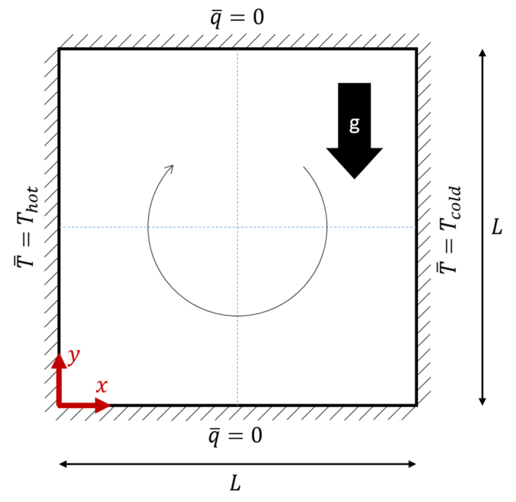
This simple 2D test case contains a square cavity in which a fluid encounters a hot wall on one side and a cold wall on the opposite side, leading to natural convection, as illustrated in Figure 2. For any choice of material parameters and experimental setup, the resulting flow and the balance between heat conduction and heat convection can be compared using dimensionless numbers, which use the thermal diffusivity, α:

$$\alpha =\frac{\kappa }{\rho c_p}$$

(37)

It has the dimension ${\mathrm{m}}^2/\mathrm{s}$ and characterizes the rate of conductive heat transfer through a medium. The first relevant dimensionless number in this case is the Prandtl number $Pr$, which reads

$$Pr=\frac{\nu }{\alpha }=\frac{c_p\mu }{\kappa },$$

(38)

where $\nu$ is the kinematic viscosity. $Pr$ describes the ratio between momentum diffusion and thermal diffusion. The second relevant dimensionless number is the Rayleigh number, $Ra$, which reads:

$$Ra=\frac{g{\beta }_V\mathsf{\Delta }T{L}^3}{\alpha \nu }=\frac{{\rho }^{2}g{\beta }_V{c}_p\mathsf{\Delta }T{L}^3}{\mu \kappa },$$

(39)

where $\mathsf{\Delta }T$ is the characteristic temperature difference and $L$ is the characteristic length scale of the problem; $Ra$ describes the ratio between convective heat transfer and conductive heat transfer. Following Aubry et al. [32], we use an edge length $L=1 \mathrm{m}$ and a temperature difference $\mathsf{\Delta }T=1 \mathrm{K}$, where the left side is arbitrarily chosen by the authors to be “hot” at $20.5 \mathrm{K}$ and the right side to be cold at $19.5 \mathrm{K}$. The authors have taken these settings from Strada et al. [37], whom they use as their reference. The dimensionless numbers are given as $\mathrm{Pr}=1$ and $Ra={10}^6$. To achieve these, we chose $\rho =1\mathrm{kg}/{\mathrm{m}}^3,$ $\mu ={10}^{-4} \mathrm{Pa} \mathrm{s},$ $c_p=1\mathrm{J}/\mathrm{kg} \mathrm{K},$ $\kappa ={10}^{-4}\mathrm{W}/\mathrm{m} \mathrm{K}, {\beta }_V={10}^{-3}{ \mathrm{K}}^{-1},$ $g=-10\mathrm{m}/{\mathrm{s}}^2$, although the other authors do not state their exact choice and their mesh specifics are also not mentioned. We use a uniform triangular mesh with an average edge length of $h=0.0125 \mathrm{m}$, and the time step is set to $\mathsf{\Delta }t=0.5 \mathrm{s}$.

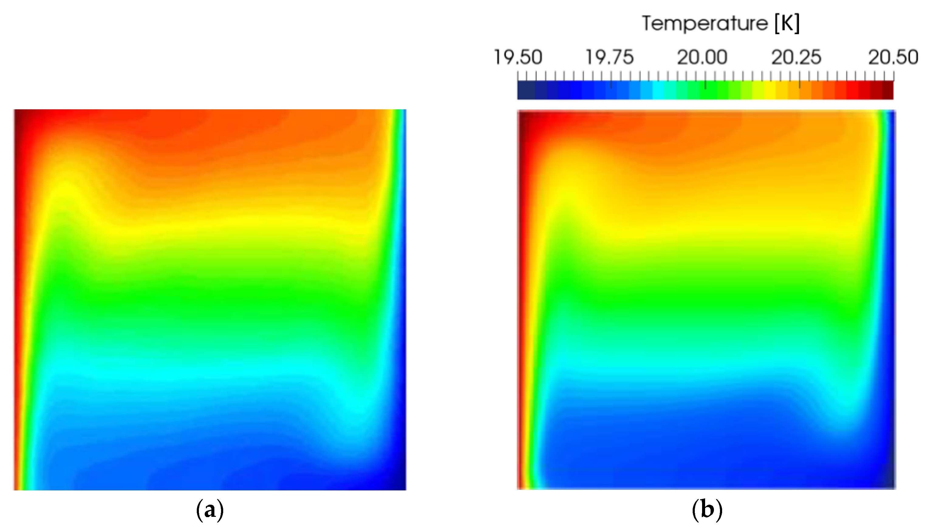
When using the same Pr and Ra, the steady state solutions are expected to match. Aubry et al. [32] reach the steady state solution after a long simulation time of 396 s. In Figure 3a, good agreement of the temperature distribution can be observed. The color maps may not match exactly, as the color distribution over the range of temperatures is not provided by Aubry et al., but the temperature fields are obviously very similar.

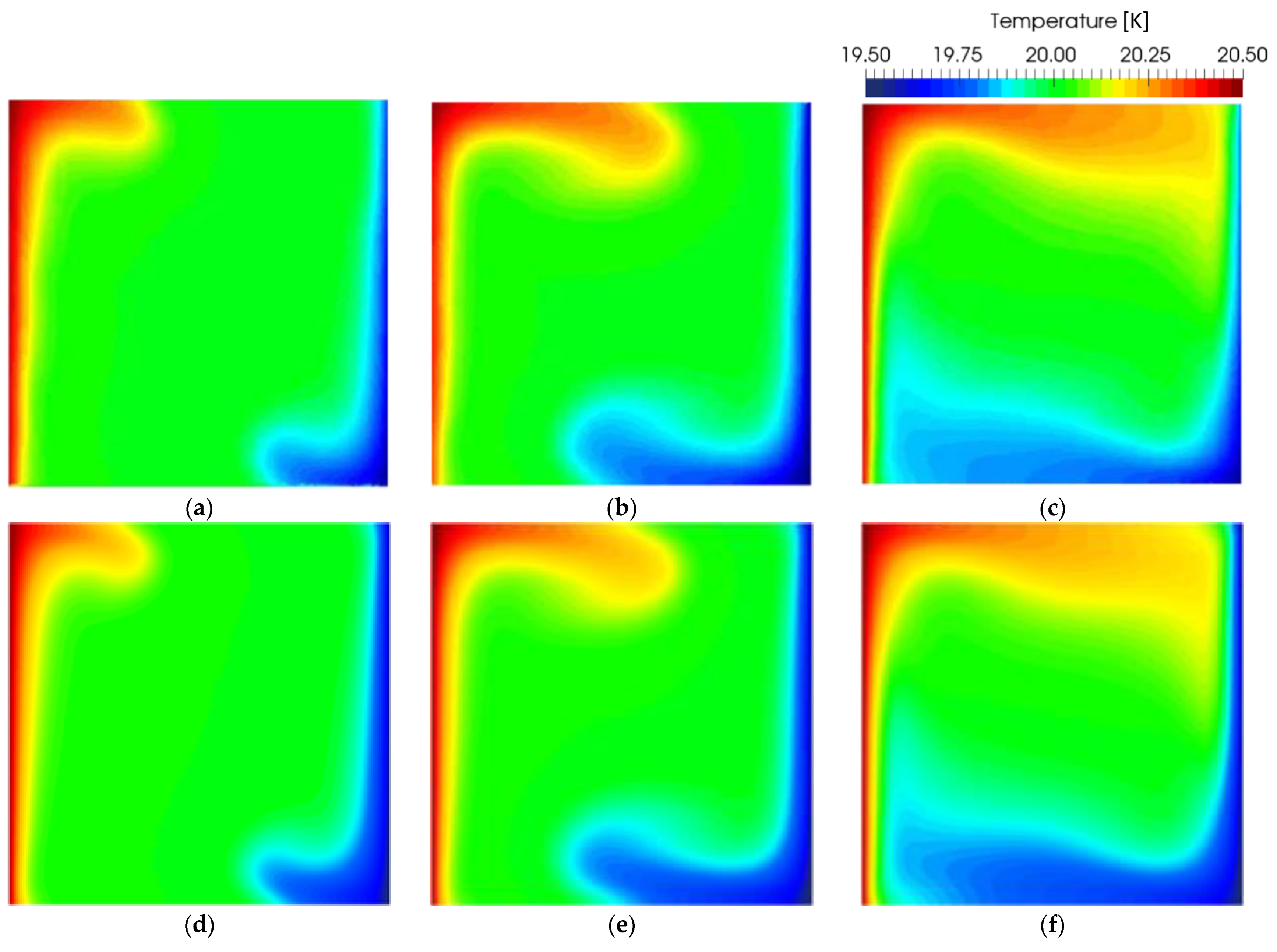
Next, the transient evolution of the temperature field before reaching the steady state is compared in Figure 4; good agreement during the whole simulation time can be observed. The gradual mixing of cold and hot fluid, along with the developing convective flow are clearly visible and no major differences can be found. It is interesting to note that a different combination of input parameters can produce the same Pr and Ra, and therefore the same steady state solution, whereas the evolution over time may be at a different rate. This can be explained by the fact that the input parameters are non-dimensional, while the time is dimensional. The use of a non-dimensionalized time, such as the one discussed in the following section, would be more appropriate. Strada and Heinrich [37], the reference used by Aubry et al., only features the steady state results; thus, no dimensionless time is required. Also note that Strada and Heinrich define Ra using K (instead of the usual α) as the symbol for the thermal diffusivity, which led Aubry et al. to accidentally define Ra with a $\kappa$, denoting thermal conductivity, in the place of thermal diffusivity, K.

An almost identical test case is presented by Marti and Ryzhakov [12], simulated with their own PFEM code. The quadratic domain still has an edge length of L = 1 m and a temperature difference of ∆T = 1 K. The main differences are that the steady state results are compared with the existing literature and that the input variables are changed. Marti and Ryzhakov first show the temperature contour plots, as above, then compare the maximum velocities encountered on the horizontal and vertical centerlines with the works of de Vahl Davis [38], Corzo et al. [39] and Sklar et al. [40]. Distance, time and velocity are non-dimensionalized as follows: non-dimensional position $\widehat{x}=x/L$ and $\widehat{y}=y/L$, a non-dimensional time $\widehat{t}=t{L}^2/\alpha$ and non-dimensional velocity $\widehat{v}=vL/\alpha$, as explained by Corzo et al. and de Vahl Davis. The other parameters used by Marti and Ryzhakov are $\rho$ = 1 kg/m³, v = 10⁻³ m²/s, α = 10⁻³ m²/s, g = −10 m/s². Furthermore, Marti and Ryzhakov mention using Pr = 0.71, while the parameters inserted into Equation (38) give Pr = 1.0, which we use in this work. The comparisons are done using Ra = 10⁴, Ra = 10⁵ and Ra = 10⁶. The uniform triangular mesh has an edge length of h = 0.015 m, the same as Marti and Ryzhakov, with a time step of ∆t = 0.5 s, ∆t = 0.05 s and ∆t = 0.005 s, respectively, for the different Rayleigh numbers in respect of the condition CFL = v_max ∆t/h < 1, and results averaged over 25 time steps after reaching the steady state.

Table 1. Resulting maximum velocities (${\widehat{v}}_{x,\max }$ and ${\widehat{v}}_{y,\max }$) on the centerlines ($\widehat{x}$ = 0.5 and $\widehat{y}$ = 0.5 respectively) and positions of maxima (${\widehat{y}}_{v_x,\max }$ and ${\widehat{x}}_{v_y,\max }$ respectively) along centerlines Ra = 10⁶. All values are non-dimensionalized.

Data $(\mathit{R}\mathit{a}={10}^6)$	this Work	Marti & Ryzhakov	de Vahl Davis	Corzo et al.	Sklar et al.
${\widehat{v}}_{x,\max }$	65.115	65.45	65.81	64.558	64.483
${\widehat{y}}_{v_x,\max }$	0.854	0.85	0.852	0.851	0.845
${\widehat{v}}_{y,\max }$	225.913	213.07	214.64	221.572	218.054
${\widehat{x}}_{v_y,\max }$	0.0404	0.0474	0.0396	0.067	0.037

,

Table 2. Resulting maximum velocities (${\widehat{v}}_{x,\max }$ and ${\widehat{v}}_{y,\max }$) on the centerlines ($\widehat{x}$ = 0.5 and $\widehat{y}$ = 0.5 respectively) and positions of maxima (${\widehat{y}}_{v_x,\max }$ and ${\widehat{x}}_{v_y,\max }$ respectively) along centerlines Ra = 10⁵. All values are non-dimensionalized.

Data $(\mathit{R}\mathit{a}={10}^5)$	this Work	Marti & Ryzhakov	de Vahl Davis	Corzo et al.	Sklar et al.
${\widehat{v}}_{x,\max }$	33.481	34.924	34.870	−	−
${\widehat{y}}_{v_x,\max }$	0.847	0.862	0.855	−	−
${\widehat{v}}_{y,\max }$	70.309	67.910	67.910	−	−
${\widehat{x}}_{v_y,\max }$	0.0700	0.0576	0.067	−	−

and

Table 3. Resulting maximum velocities (${\widehat{v}}_{x,\max }$ and ${\widehat{v}}_{y,\max }$) on the centerlines ($\widehat{x}$ = 0.5 and $\widehat{y}$ = 0.5 respectively) and positions of maxima (${\widehat{y}}_{v_x,\max }$ and ${\widehat{x}}_{v_y,\max }$ respectively) along centerlines Ra = 10⁴. All values are non-dimensionalized.

Data $(\mathit{R}\mathit{a}={10}^4)$	this Work	Marti & Ryzhakov	de Vahl Davis	Corzo et al.	Sklar et al.
${\widehat{v}}_{x,\max }$	15.948	16.250	16.182	16.282	15.982
${\widehat{y}}_{v_x,\max }$	0.820	0.821	0.823	0.822	0.824
${\widehat{v}}_{y,\max }$	19.551	19.541	19.509	19.547	19.378
${\widehat{x}}_{v_y,\max }$	0.120	0.115	0.120	0.123	0.116

show good agreement between our results and those reported in the literature. The differences lie somewhat in the range of the fluctuations between the various results in the literature. The best agreement was expected with Marti and Ryzhakov, as they used the same method and the same mesh. De Vahl Davis and Corzo et al. used different simulation methods, the Finite Difference Method (FDM) and the Finite Volume Method (FVM) respectively, both of which use Eulerian formalism.

The temperature contours obtained were also compared with those shown by Marti and Ryzhakov, with good agreement observed (not shown here).

3.2. Buoyancy and Marangoni-Driven Convection in a Square Cavity

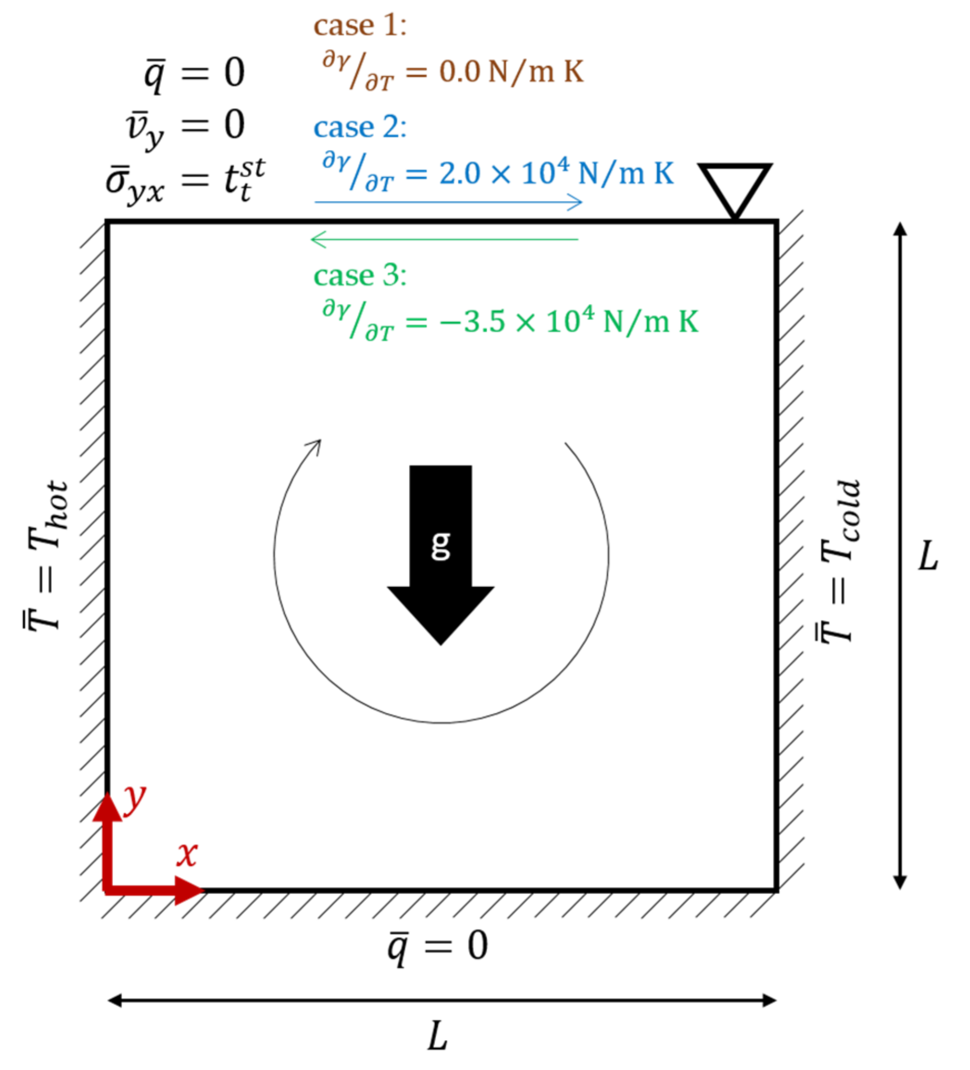
This 2D test case also uses a square cavity with a buoyancy driven flow, as above, but with additional surface tension acting on the top surface, see Figure 5. Comparisons are done with literature results from Saldi’s PhD thesis from 2012 [33], who himself uses older results from Bergman and Keller from 1988 as a reference [34]. Since all the authors use a Eulerian Finite Volume Method, the top surface is assumed to remain flat, limiting the effect of surface tension to the tangential component, which is referred to as the Marangoni effect. Three test cases are investigated; the first one does not include the Marangoni effect, recovering a test case similar to those in the previous section. The second test case includes a negative Marangoni coefficient $\partial \gamma /\partial T$, causing the Marangoni effect to push fluid at the surface in the same direction as the circulation caused by the underlying buoyancy-driven convective flow, reinforcing the circulation. The third case uses a positive $\partial \gamma /\partial T$, leading to an opposite effect where the surface tension pushes against the underlying buoyancy-driven flow, counteracting the circulation at the surface.

The material data are given in detail by Bergman and Keller, resembling molten aluminum at 660 °C: $\rho$ = 2385 kg/m³, μ = 1.3 × 10⁻³ Pa s, c_p = 1080 J/kg K, $\kappa$ = 94.03 W/m K, β_V = 1.17 × 10⁻⁴ K⁻¹. This gives us Pr = 0.0149 and Ra = 4.6 × 10⁴. These settings fully describe case 1, where only the buoyancy effect is driving the flow. For the other cases we superimpose the Marangoni effect; thus, the Marangoni number Ma (sometimes denoted as Mg to avoid confusion with the Mach number) that describes the relative importance of the Marangoni effect compared to the viscosity is defined as

$$Ma=\frac{\raisebox{1ex}{$\partial \gamma $}\!\left/ \!\raisebox{-1ex}{$\partial T$}\right. \mathsf{\Delta }TL}{\alpha \mu }=\frac{\raisebox{1ex}{$\partial \gamma $}\!\left/ \!\raisebox{-1ex}{$\partial T$}\right. \rho c_p\mathsf{\Delta }TL}{\mu \kappa }.$$

(40)

The Marangoni coefficient is $\partial \gamma /\partial T=2.0\times {10}^{-4}\mathrm{N}/\mathrm{m} \mathrm{K} \mathrm{for} \mathrm{case} 2$ and $\partial \gamma /\partial T=-3.5\times {10}^{-4}\mathrm{N}/\mathrm{m} \mathrm{K}$ for case 3. This results in $Ma=0$, $Ma=1.47\times {10}^4$ and $Ma=-8.4\times {10}^3$ for cases 1, 2 and 3, respectively. The cavity has an edge length of $L=0.02 \mathrm{m}$ and a Temperature difference $\mathsf{\Delta }T=100 \mathrm{K}$ between cold and hot walls. All results are compared after reaching steady state equilibrium. We use an element size of $\mathsf{\Delta }x=0.001 \mathrm{m}$ and a time step of $\mathsf{\Delta }t=0.001 \mathrm{s}$, $\mathsf{\Delta }t=0.0005 \mathrm{s}$ and $\mathsf{\Delta }t=0.0005 \mathrm{s}$ for the three cases, respectively, to accommodate the higher local velocities produced by the Marangoni effect. Further refinement of the time step mesh size does not improve the results. Saldi uses a Eulerian FVM approach, and does not state mesh size or time step length. Bergman and Keller use a steady state Eulerian FVM approach with a similar mesh size, but with a refinement near the boundaries.

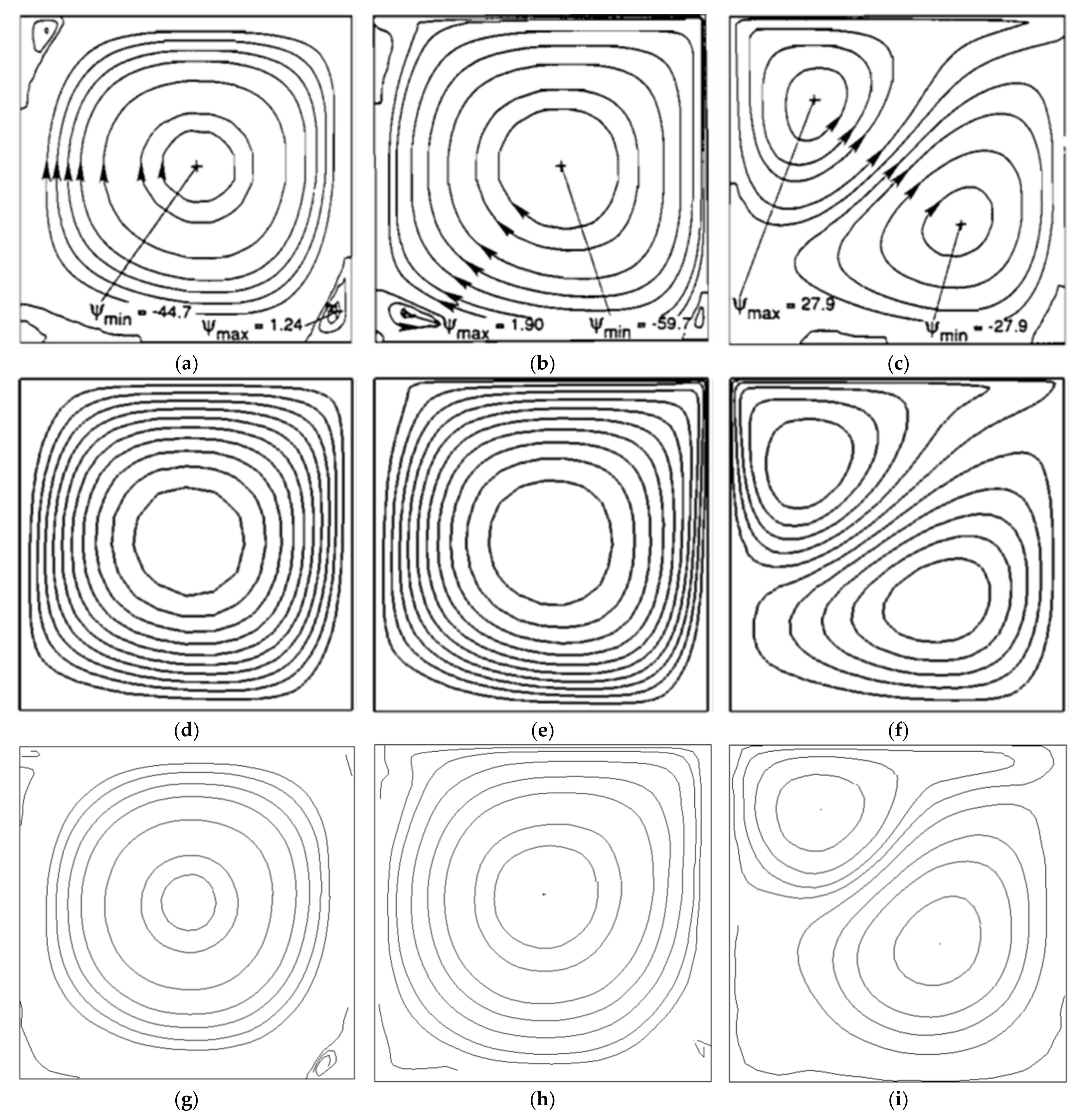
Both Saldi [33] and Bergman and Keller [34] compare streamlines that highlight the flow pattern for each case. As we do not have the stream function (see e.g., [41], p. 14) available in our results, we constructed the streamlines by integrating from a given seed point in space over the velocity vector field. For this approach, the seed points must be chosen by the user, and the resulting streamlines do not necessarily represent the same value of the stream function as given by Bergman and Keller. We chose each seed point at a location that is intersected by the streamlines from Bergman and Keller in an attempt to produce the most qualitatively similar representation of the main flow field. For the recirculation bubbles that can appear in the corners, we freely chose a convenient location for the seed points with the aim of best capturing the flow pattern in the corners. Crucially, these different procedures for obtaining the streamlines introduce some uncertainty when comparing streamlines. The comparison between Bergman and Keller (top), Saldi (middle) and our work (right) can be found in Figure 6.

The results show good overall agreement, although a few discrepancies can be found as well. For case 1 in Figure 6a,d,g, the main flow fields are nearly indistinguishable. Small differences can be found with the recirculation bubbles in the corners, and no bubble is found in the bottom left corner at all. Such recirculation bubbles are, however, naturally rather unstable and sensitive to the main flow field. Good agreement regarding the size and position of cells of slow-moving fluid and reversed flow can be seen.

For case 2 in Figure 6b,e,h, the effect of the surface tension enhancing the underlying buoyancy-driven circulation can be seen. The streamlines reach much further into the top right corner before changing direction, and the streamlines there also come closer together. Otherwise, the flow pattern is largely the same as in case 1. The agreement is better between Bergman and Keller (b) and Saldi (e) than with our results (h). Again, we find slightly different recirculation bubbles in the corners, and the vortex center of the main circulation is more centered in (h) than in (b) and (e).

For case 3, in Figure 6c,f, the surface tension can clearly be seen counteracting the buoyancy, as the flow pattern is neatly divided into two distinct vortices. A line of zero vorticity, where the two vortices meet, would occur close to the diagonal between bottom left and top right corner. This flow pattern is found to be sensitive to Ra and Ma, such that a small change in input parameters would quickly favor one of the two effects over the other, quickly leading to one of the main vortices to dominate over the other. It is possible that this delicate balance was deliberately chosen by Bergman and Keller to emphasize the importance of the Marangoni effect, as they argue that the Marangoni effect has been largely neglected in applications where convective flows in liquid metals are of importance. The agreement of all three results is less good than before, and the size and position of the two distinct vortices is slightly different in each case. Given the delicate balance that causes this flow pattern, our result agrees well with the literature, as the differences are very minor.

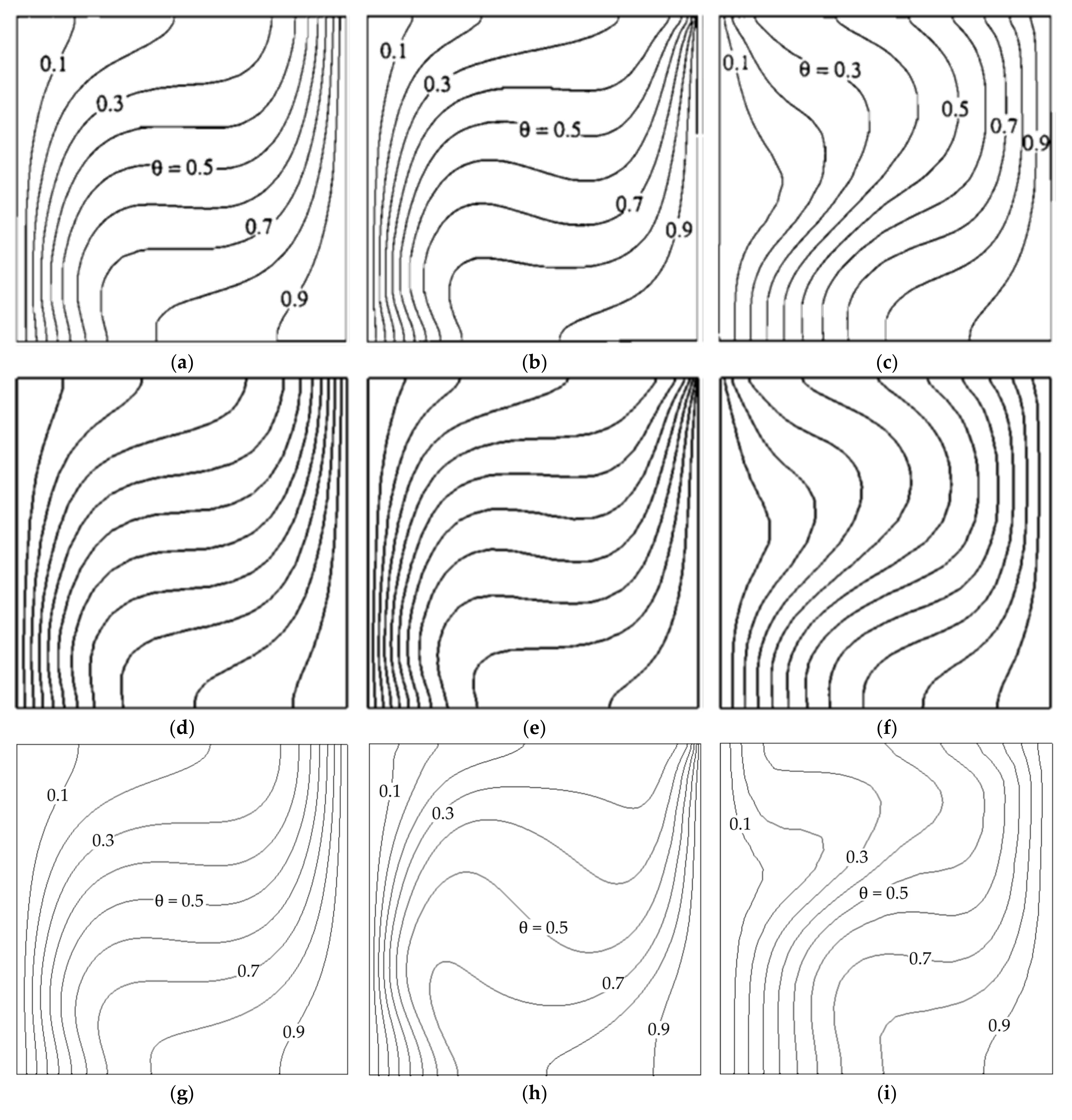
Both Saldi [33] and Bergman and Keller [34] also present plots of isotherms using a non-dimensionalized temperature θ = (T − T_min)/∆T with a spacing of 0.1. The agreement between all three publications is good. Comparing Bergman and Keller’s result in the top row of Figure 7 with Saldi’s in the middle and ours on the bottom row, a similar tendency as in the previous comparison can be observed: qualitatively a good agreement when looking at the overall appearance of the plots; the spacing of the isotherms in most cases is especially well captured, indicating that the important temperature gradients are well-captured. On the other hand, several discrepancies can be found for cases 2 and 3 between literature results in Figure 7b,e and Figure 7c,f and our results Figure 7h,i respectively. In both cases 2 and 3, the isotherms appear more twisted in a clockwise direction in the areas where the convective flow is strongest. Unfortunately, no experimental results that can validate the simulation results from the literature could be found, which leaves some uncertainty regarding any of the results presented.

3.3. Melting of a Block of Gallium

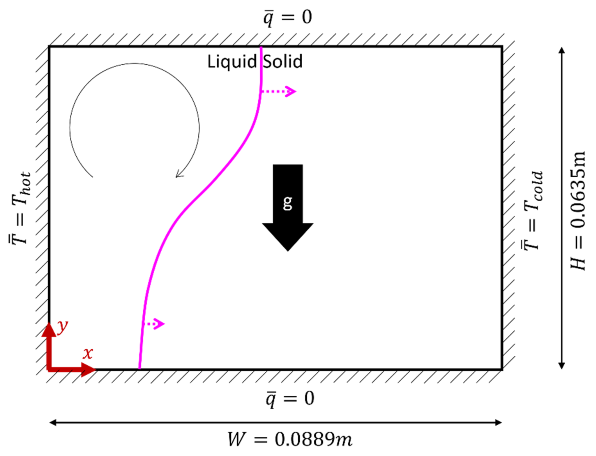
A rectangular block of solid gallium slightly below the melting point is in a closed box. The block is exposed to a hot wall on the left, which is of constant temperature significantly above the melting point. The gallium then progressively melts from left to right. This test case combines a buoyancy-driven convective flow and the modelling of phase change, which affects momentum equation and heat. All of these effects are strongly coupled, leading to an interesting test case. A schematic is provided in Figure 8.

This test case is based on experiments originally conducted by Gau and Viskanta in 1986 [35]. The advantage of choosing gallium is that the melting point, Tm = 302.78 K, is near room temperature, greatly simplifying the experimental setup. Likewise, a pure metal exhibits a sharp melting front, which is easier to measure. The remaining material parameters are $\rho$ = 6093 kg/m³, μ = 1.81 × 10⁻³ Pa s, c_p = 381.5 J/kg K, $\kappa$ = 32.0 W/m K, β_V = 1.2 × 10⁻⁴ K⁻¹ and ∆h_L = 8,016,021 J/kg. 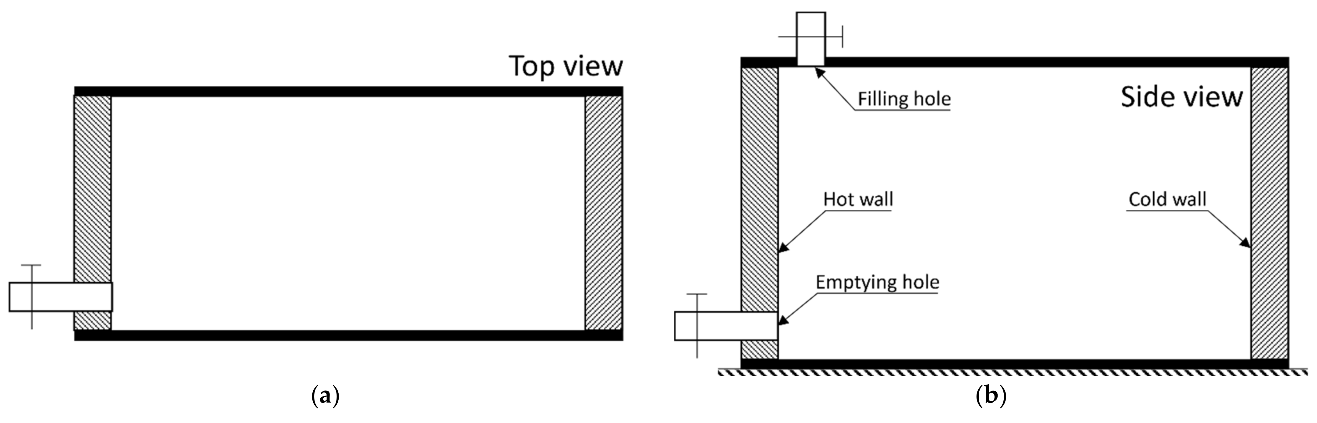The hot wall on the left has T_hot = 311.0 K, and the cold wall on the right has T_cold = 301.3 K, which is also used as initial temperature T₀ from the entire domain. Note that the initial temperature is very close to the melting point. The experimental setup is shown in Figure 9. The cavity can be adjusted to have different dimensions, resulting in different aspect ratios A = H/W, where H = 0.0635 m and W = 0.0889 m are typically used for the height and width of the cavity, respectively, to arrive at an aspect ratio of A = 0.714. This aspect ratio is used in the simulations described below, and other aspect ratios mentioned by Gau and Viskanta are ignored in this work.

The process of obtaining the position of the melting front in the experiment is not simple, as gallium is not visually transparent. First, melted gallium is poured into the cavity through the opening at the top, which is sealed afterwards. Then, the entire cavity is cooled down to the initial condition, which is a fixed temperature slightly below the melting point. At this stage, the gallium has completely solidified in the cavity. The experiment begins by pushing fluid of a constant given temperature through the side walls, the left one hot and the right one cold; this way, the side walls maintain a constant temperature throughout the entire experiment. As time passes, the gallium melts near the hot wall and convective flow sets in. After a given time, the experiment is interrupted and the liquid quickly evacuated from the cavity, leaving only the remaining solid part of the gallium block behind. From this block, the melting front is traced and photographed. For each time duration, the experiment is repeated from the beginning to finally reconstruct the progression of the melting front over time. This way, the melting front position is obtained for nine different time marks (2, 3, 6, 8, 10, 12.5, 15, 17 and 19 min). It is not disclosed if the experiment was repeated several times and the results averaged for each time mark. It is also not discussed in detail how the experiment could be flawed. Potential issues can arise from:

• 3D effects that are not represented in the 2D curves of the melting front;
• Shrinkage after filling the cavity with liquid gallium and letting it solidify, leading to potential loss of contact between the gallium and the walls;
• Heat losses or parasitic heat conduction in the walls;
• Possible transient temperature evolution in the “constant temperature walls” upon switching on the constant temperature liquid feeding system;
• Possible continuation of the melting while the liquid is evacuated too slowly, leading to sloshing potentially affecting the roughness of the resulting surface;
• Possible errors from tracing and photography, not explained in detail.

Another large uncertainty is introduced through the strong anisotropy of the thermal conduction of solid gallium. This issue is discussed in the work Gau and Viskanta in the context of the inverse experiment, where the gallium is initially liquid and then solidified on a constant temperature cold wall, as opposed to the melting of solid gallium on a hot wall, which is the topic of this work. In the solidification experiment, the physical behavior has been found to be highly dependent on the crystallography of the freshly solidified gallium, introducing significant variability into the position of the solidification front. In the melting experiment, the authors explain that the anisotropy of the solid gallium plays a lesser role, as the physical behavior is dominated by the heat transfer in the liquid, which is plausible. However, a quantitative evaluation of the variability of the experiment should have been included. It is also not clear if the presented results were obtained through several repetitions and subsequent averaging.

In 1988, Brent et al. [36] attempted to match the experimental results with a Eulerian Finite Volume Method approach that used an extremely coarse mesh by today’s standards. The latent heat absorption was accounted for using an iterative nodal enthalpy formulation that also works on coarse, fixed grids. The authors point out that this scheme creates a diffuse phase change region rather than a sharp front. The momentum equations are modified for the solid using the same Carman–Kozeny equation for porous media as in Section 2.5. This combination of nodal enthalpy with an iterative scheme for the phase change and the porosity model for the solid is called the enthalpy–porosity approach in their work. The authors model the experiment as closely as possible, using the same material properties and a fixed rectangular domain with an aspect ratio A = 0.714. The boundary conditions at all walls are no-slip conditions. The authors provide results on streamlining and temperature contour plots for four time marks (3, 6, 10, 19 min) as well as the melting front position for all nine time marks, as was done for this experiment.

More recently, Saldi [33] also used a Eulerian Finite Volume Method approach with the same Carman–Kozeny equation to freeze the fluid’s motion as in Section 2.5. For the latent heat, Saldi uses a separate source term calculated using an iterative scheme similar to the one used by Brent et al. [36]. Saldi’s work unfortunately does not state what numerical parameters (such as time step size, mesh size or residual target) were used. It is also not clear which type of boundary conditions were used on the walls.

The latest research publications that feature this test case tend to use it as a validation step. Unfortunately, this means that these publications provide neither an exhaustive description of the setup, nor an in-depth discussion of the results. We have picked two recent publications that highlight the variability of numerical results. First, Tiari et al. 2021 [42], who use the commercial FVM fluid dynamics code Ansys, with a mesh resolution between 12,500 and 50,000 elements. Secondly, Sharma et al. 2021 [43], who use the commercial (Eulerian) FEM code COMSOL. The equations to be solved are clearly described, but no further details about the simulation setup are given in either reference.

Our simulation setup is shown in Figure 8. Several mesh densities were tested to determine the required mesh resolution, as further discussed below. It was found that an initial mesh with 61 × 85 = 5185 nodes and 10′080 triangular elements is sufficiently fine to adequately capture the main features of the solution. Further refinement does not improve the results. A constant time step of ∆t = 0.02 s was used, which requires 57,000 time steps to complete 19 min of real time. The normalized residuals for momentum and heat equation must reach a threshold of ${\epsilon }_{crit}={10}^{-6}$. The width of the regularization was chosen to be ∆T_pc = 0.4 K, which is a close approximation of the step function, although not the smallest value that we could achieve before encountering convergence issues. The results shown below were obtained with an adaptive mesh refinement, where the regions of the mesh that are solid and far from the melting front were allowed to be coarsened by a factor of ten.

The top boundary was originally modelled with a no-slip boundary condition, the same as all other walls. This was specifically described by Brent et al., whereas other authors do not explicitly mention it. Alternatively, we repeated the simulation with a free slip boundary condition at the top. This choice is discussed below.

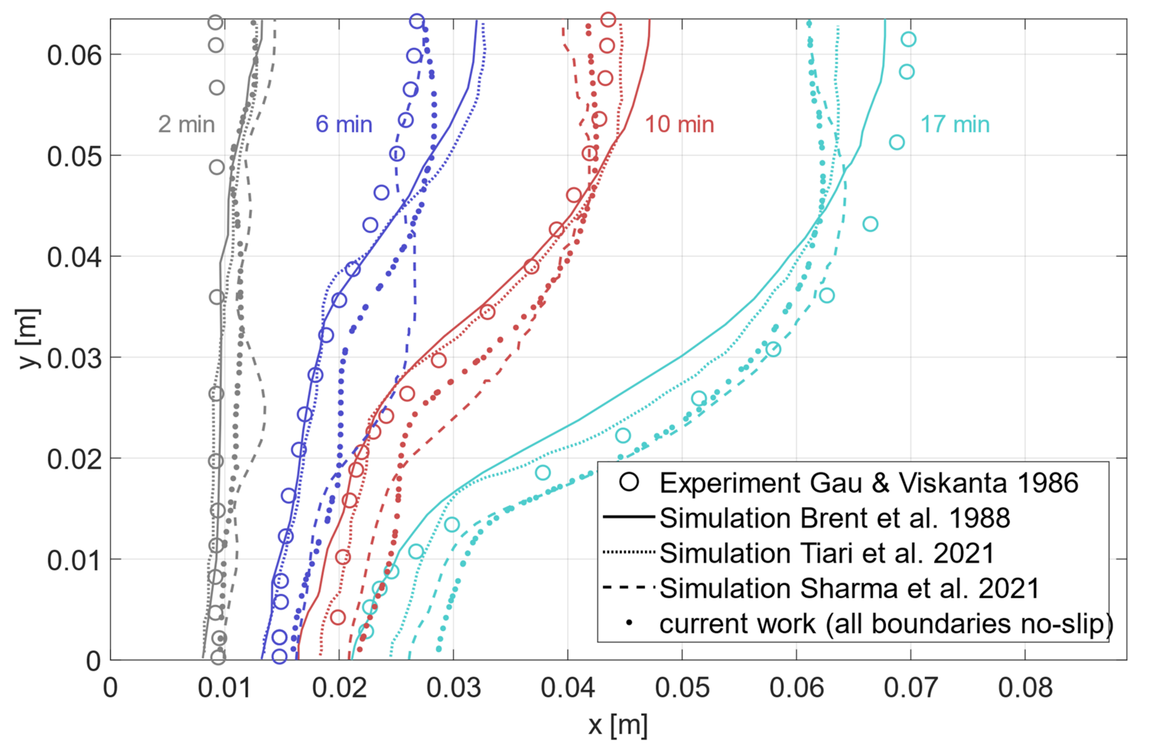
A comparison of the position of the melting front at four time instances with the original no-slip boundaries is found in Figure 10. None of the methods agree perfectly with the experiments by Gau and Viskanta, but all show at least the same overall behavior: The melting front is faster near the top, as the heat transfer is convection-dominated there. This effect becomes more pronounced over time. Conversely, the bottom advances considerably more slowly due to the reduced influence of the heat convection compared to heat conduction, which dominates there. These effects combine to produce the curved shape of the melting front.

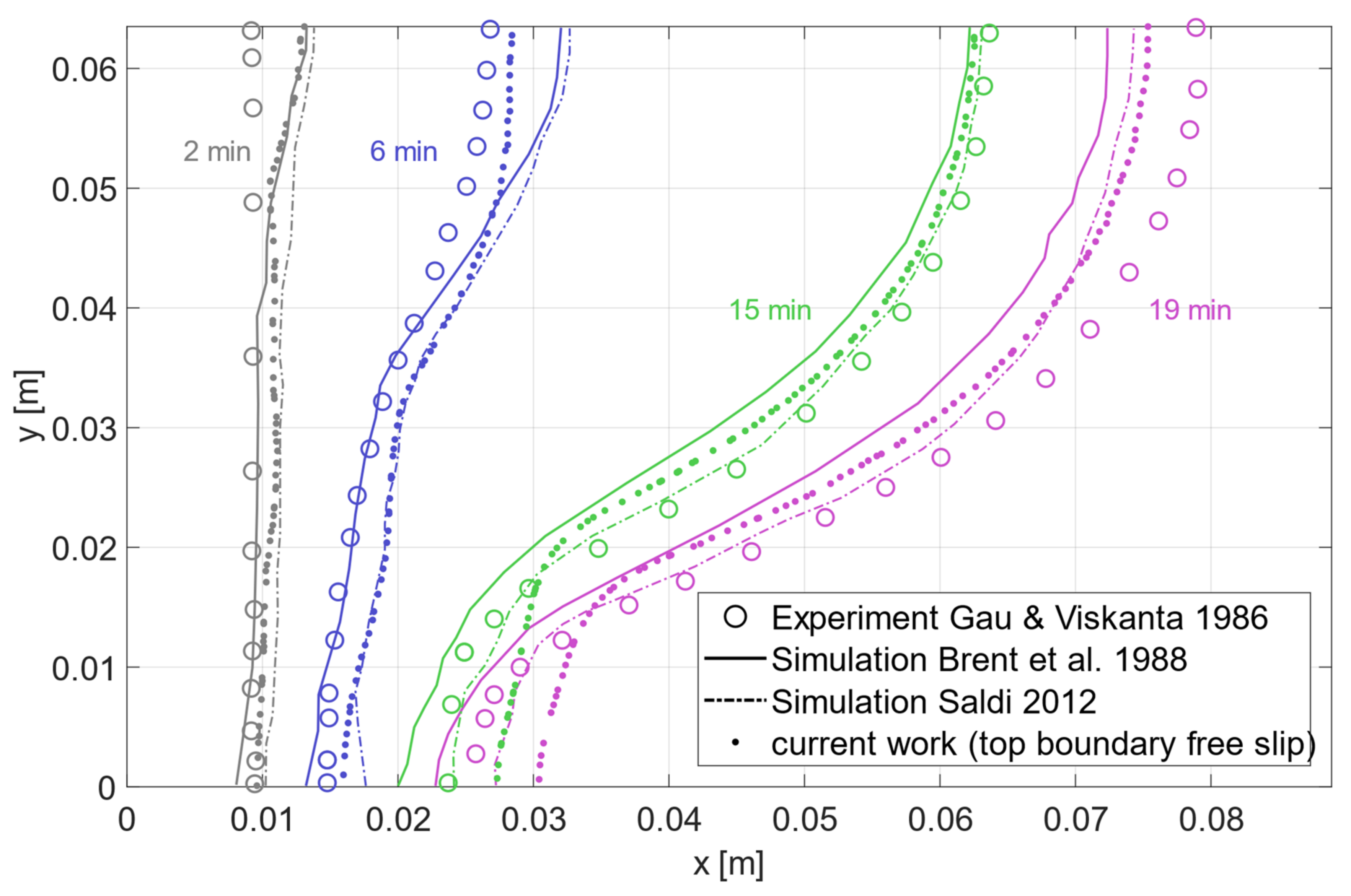
Evidently, this creates a shape of the curve that does not agree well with the experiments. One finds a backwards curved front near the top boundary that is not observed in the experiments. When instead switching to a free slip boundary at the top, the results seem to agree better with the experiments, as shown in Figure 11. With the original no-slip condition, the advancement of the front is slowed near the top surface. A hypothetical explanation regarding the experimental results relies on the strong assumption that the top surface of the liquid gallium may not be in contact with the casing during the experiment due to shrinkage. We cannot know if this was the case during the experiments; however, the possibility persists, and our results improve noticeably with this boundary condition. An alternative justification could be a thin boundary layer that is best modelled by a free slip condition; however, assuming a laminar flow, the mesh that we use seems to be sufficiently fine. More work is needed to confirm or reject this assumption. We also see this shape in the results by Saldi [33] and Brent et al. [36], although there is no reason to assume that a free slip condition was used at the top boundary.

In general, we observe the same overall behavior in all cases: At the 2-min mark, all simulation results seem to have the same tendency of a rather straight vertical melting front that exhibits a slight shift to the right at the very top. This effect is not observed in the experiments. After 6 min, when the problem transitions from conduction-dominated to convection-dominated, the greatest dispersion of results is observed. While the experiments start to show the effect of the convective heat transfer in the top half of the domain, where the front position is slightly shifted to the right, the simulations all tend to overestimate the advancement of the melting front. At later time instances (10, 15, 17, 19 min) all simulation results agree much better with the experimental result, as the curves have the more or less correct shape and advancement in the x-direction. This can be explained by the stable vortex structure that has formed at these times, as discussed in following paragraphs.

Some explanations for the above observations can be drawn from a more detailed look at the velocity and temperature field. No such information is provided in the experimental work of Gau and Viskanta [35], and details provided about the simulation results of Saldi [33] and Brent et al. [36] are scarce. Tiari et al. [42] and Sharma et al. [43] do not provide any deeper insight into the velocity and temperature fields. The flow field at the beginning is characterized by a narrow vertical column of fluid between the hot left wall and the comparably cold melting front, which is advancing evenly towards the right. This column of fluid, with its large temperature gradient, immediately begins to develop a circulation driven by buoyancy. The circulation forms into several separate circulation cells or vortices. When the width increases over time as more material is continuously melted, the size of the vortices increases, which means that the number of vortices that can fit in the height of the fluid column must decrease over time; this process thus begins with many small vortices and develops into few large vortices.

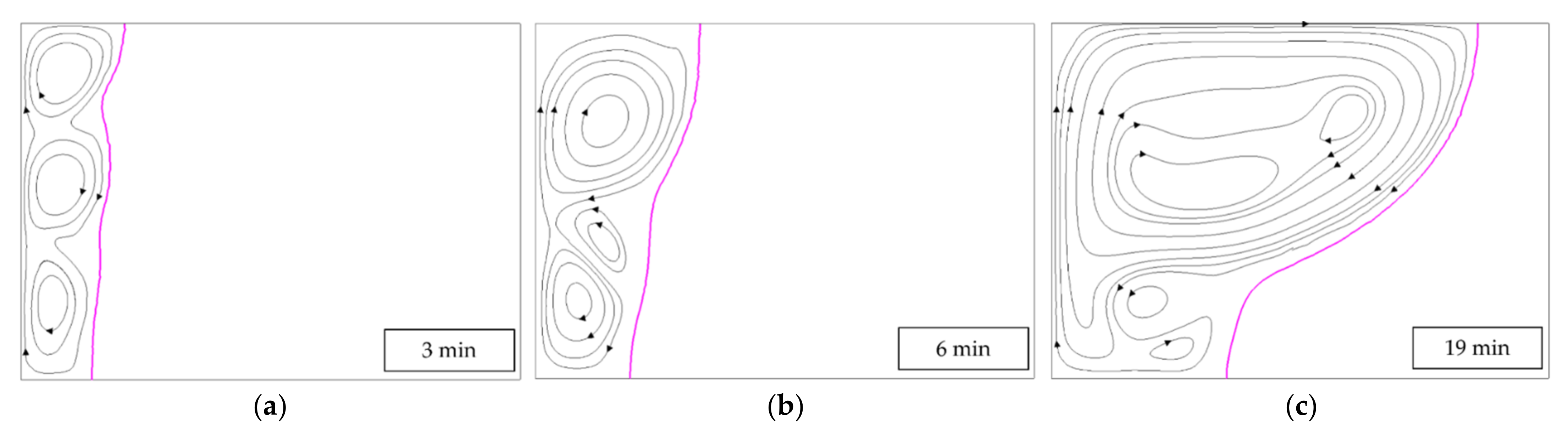
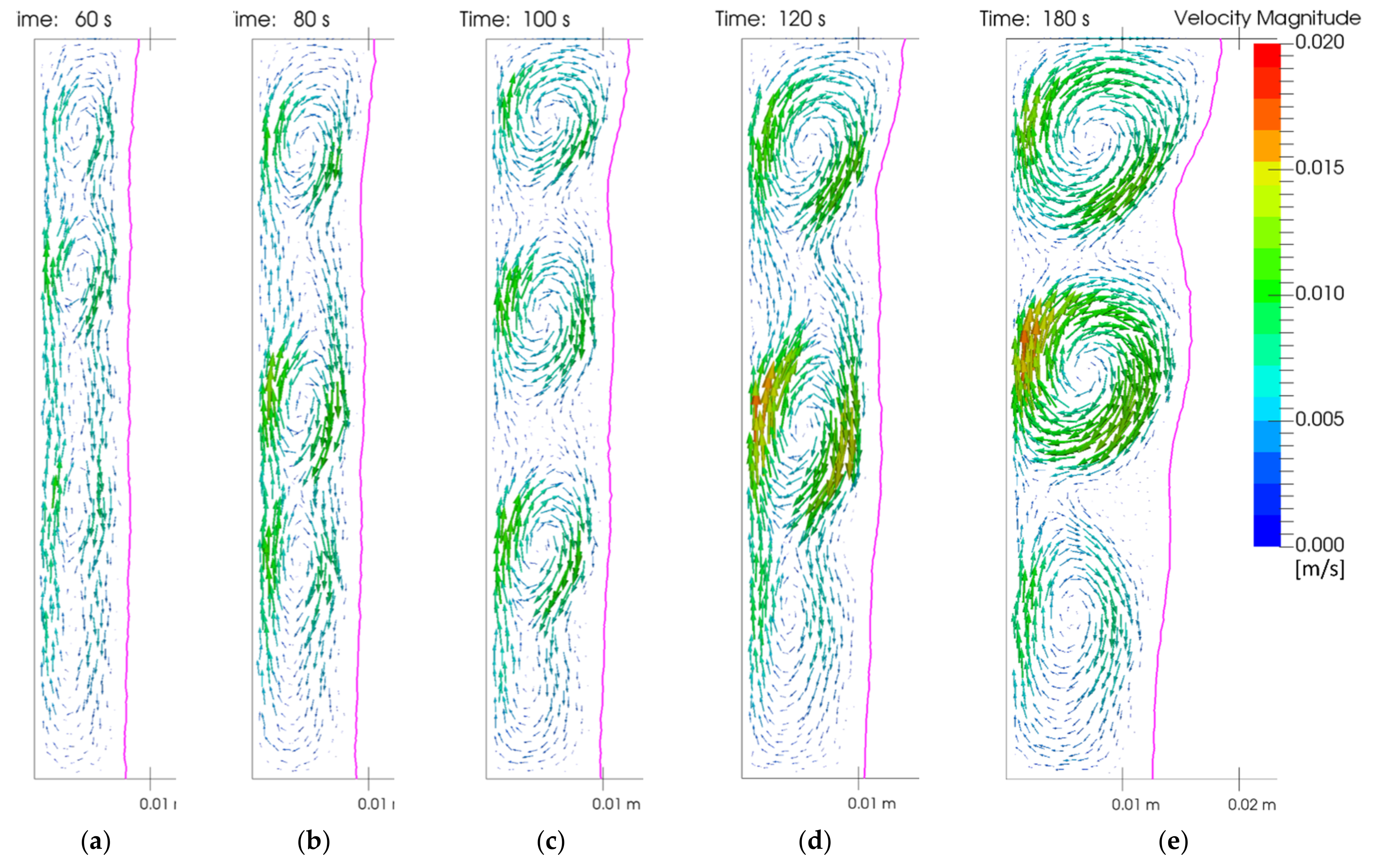
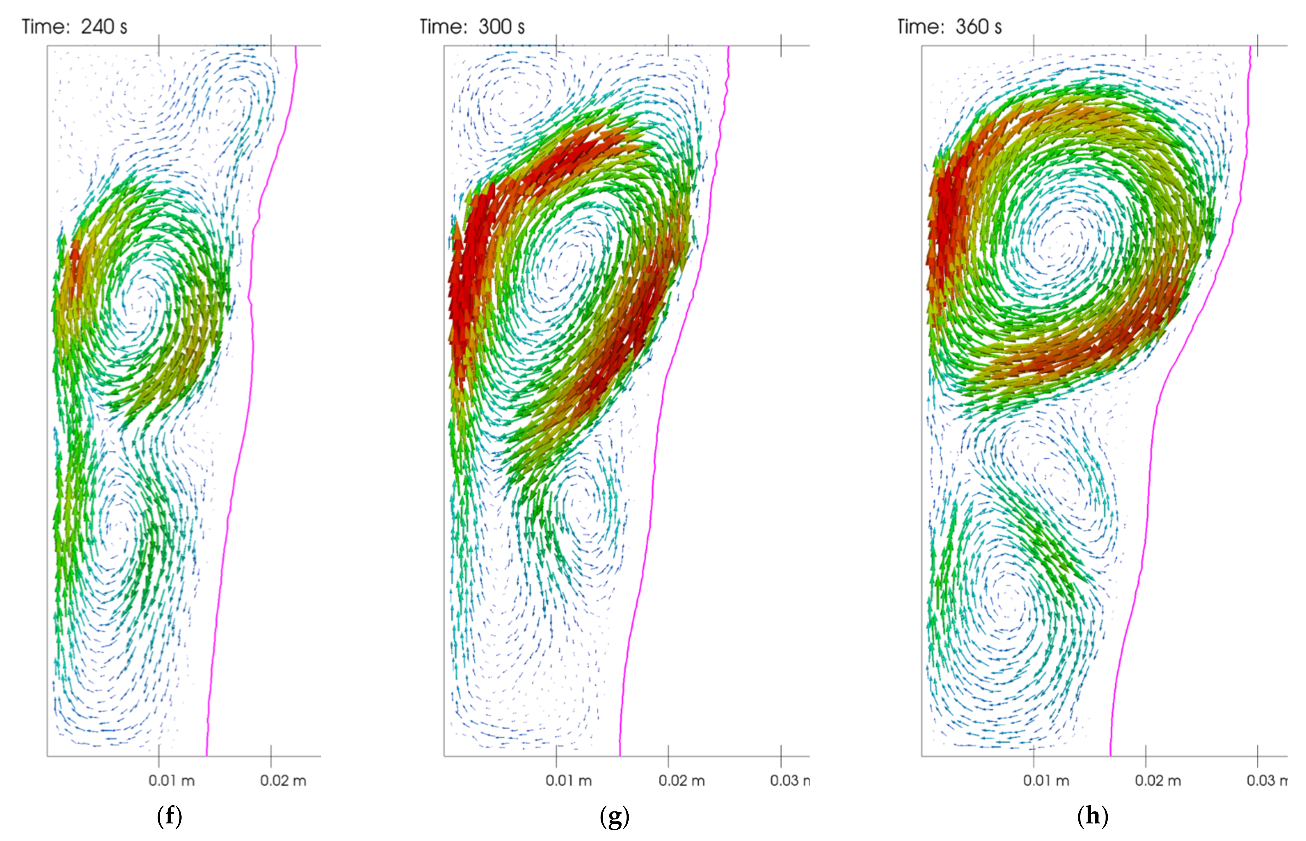
The development of the vortex structure over time can be analyzed using Figure 12. It is at around 60 s (a) that the vortices establish themselves for the first time, in this case three distinct vortices and three transition regions where the fluid motion is less pronounced. Shortly after, at 80 s (b), the dominant vortices are found to be more compact and more round, creating more space at the bottom, where a fourth vortex is in the process of establishing itself. Before it can fully develop, the entire flow field collapses and two dominant vortices emerge after 100 s (c). Again, the vortices grow more compact, faster and more circular, allowing a weak vortex at the bottom to grow into a fully developed one, as apparent after 120 s (d). This flow structure gains further momentum and stabilizes itself at 180 s (e), before it begins collapsing after 240 s (f), where a completely different flow field has emerged. In the transition between 180 s and 240 s, the two strong vortices at the top have merged temporarily into one vortex that shortly afterward gives rise to another weak vortex, which can be seen in (f). From there on, the final more stable flow field develops, as the strong vortex in the middle becomes more and more dominant, as evident in (g) and (h). Note that all vortices literally carve concave cavities into the remaining solid over time. As a result, the phase front is never perfectly straight and constantly evolves in a curving fashion according to the flow pattern. Conversely, the only reason the front remains mostly straight for so long in the beginning is because the vortices shift around, collapse and reappear so vigorously and frequently that no vortex ever stays in one position for long, therefore not getting the time to carve deeper into the solid.

This process of vortex formation and collapse between 1 min and 5 min is found to be strongly mesh-dependent, as each slight modification can produce a very different evolution of the flow field. There is no tendency that a mesh refinement necessarily converges to some sort of final result. However, for the flow field after 5 min when the main vortex has established itself, mesh dependence is no longer observed. As for the effect on the position of the melting front shown in Figure 10, there is a delay of 1–2 min after a given vortex pattern has established itself. This explains the discrepancies at the 6 min mark, as the curve in Figure 10 depends on the vortex configuration at 4–6 min.

When directly comparing the flow field at the 2 min mark in Figure 12d to Saldi’s vector plots in Figure 13, one can see that the best match is obtained with the coarse mesh in Figure 13a. This may not be surprising at first, as the presented results are obtained on a mesh that is coarser than any of the ones used by Saldi. However, from the evolution over time in Figure 12 it becomes apparent that choosing a snapshot at one single time instance does not describe the flow very well due to how rapidly the flow field changes. Whether Saldi’s solution features the same rapid and chaotic development of the vortex structure over time cannot be deduced from the single snapshot that is provided.

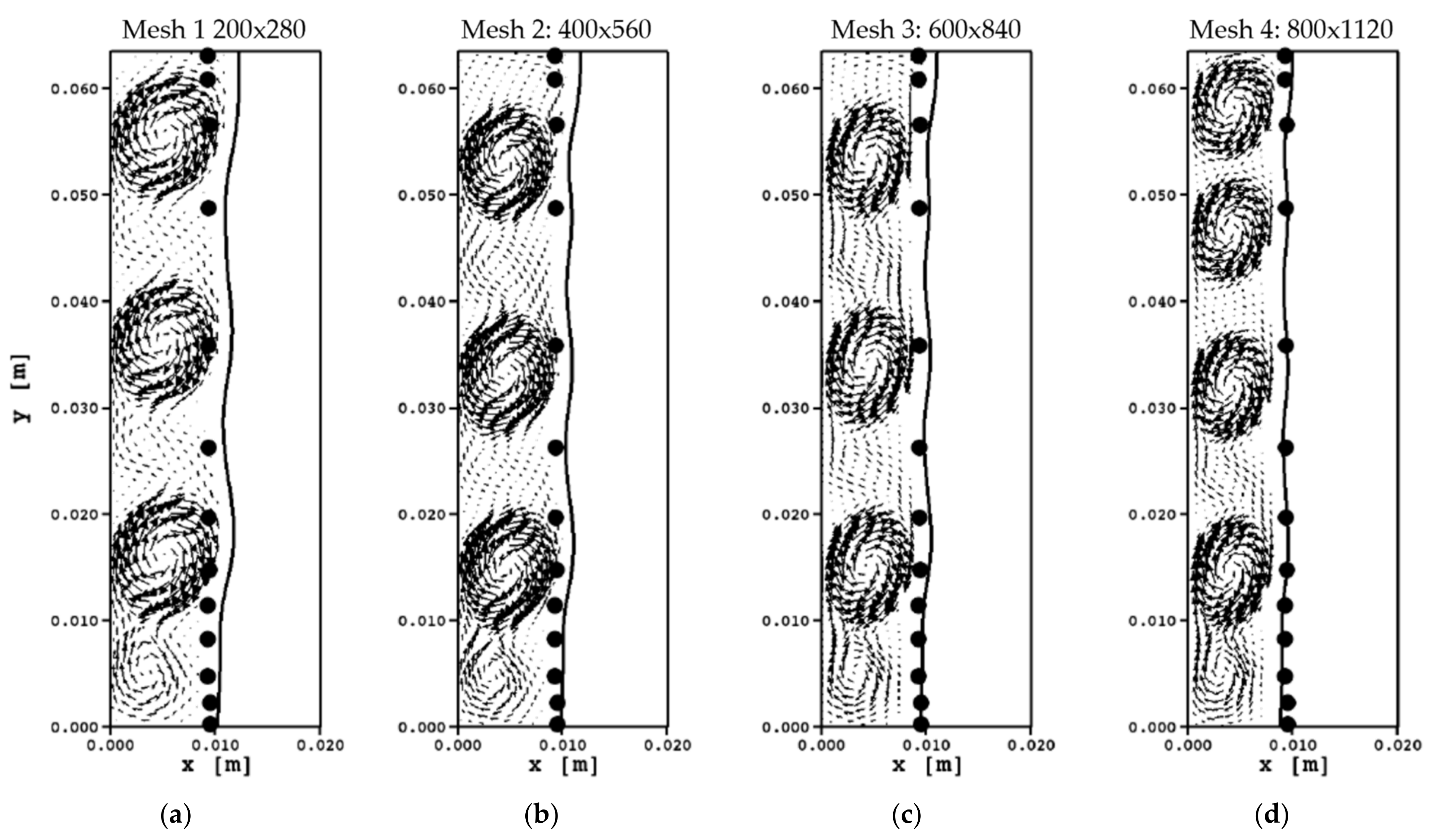
Saldi’s plots are instead intended to show the mesh dependence of the early solution. Upon further refinement, the flow field changes completely. Instead of 3 well developed vortices, the fine mesh in Figure 13d produces 4 vortices. The effect of this is an even straighter phase front as with the coarser mesh, which, as pointed out by Saldi, agrees better with the experiments (black circles). However, for the results in Figure 10 Saldi seems to use one of the coarser meshes (Figure 13a–c or even coarser), since the melting front at the 2-min mark in Figure 10 is curvy and shifted slightly to the right. Brent et al. 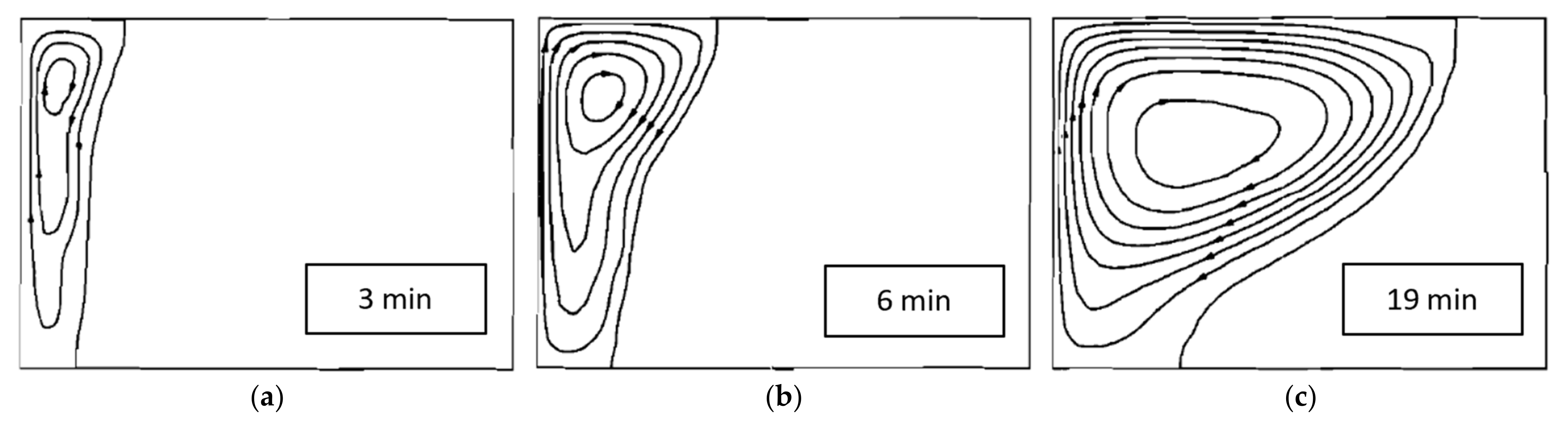[36] use an even coarser mesh of 42 × 32 cells, which is not sufficient to resolve the vortex structure found in the other simulations. In fact, there seems to be only one vortex that covers the entire liquid region at all times in Figure 14. Unfortunately, a direct comparison with Saldi is not possible, as Saldi only provides details about the flow field at 2 min, while Brent et al. provide details for 3 min and later (Figure 14a). Nevertheless, it can be clearly concluded that the extremely coarse mesh does not resolve the physics of the flow well. It is also remarkable that Brent et al. seem to generally produce rather small velocity gradients, which we do not observe (see Figure 15). Our streamlines also show steeper gradients and relatively large vortex centers.

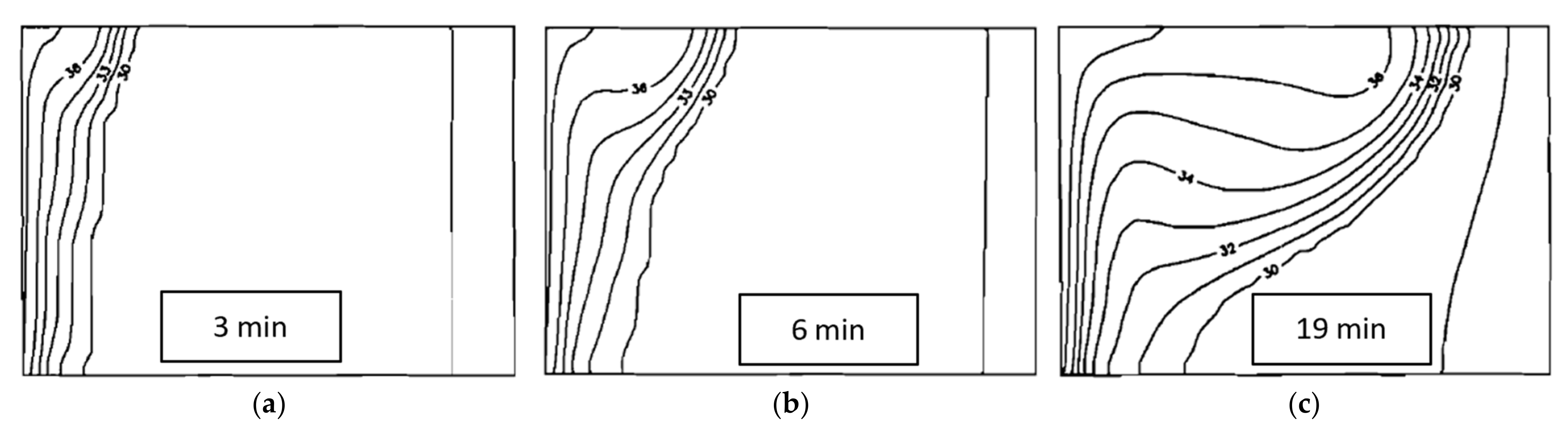
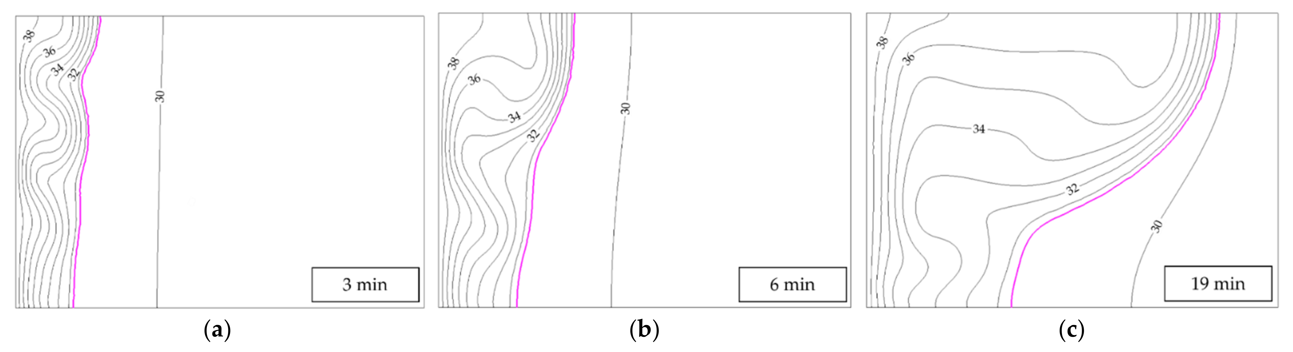
Likewise, in the results of Brent et al. the isotherms in Figure 16 reflect the smoothness of the flow field, as they are not strongly twisted or curved. Our results clearly show the influence of the flow on the temperature field, as isotherms are twisted by the vortices and re-circulation bubbles (Figure 17).

In summary, neither the streamlines nor the isotherms agree well. The explanation is that the simulations by Brent et al. use such a coarse mesh that all the details of the complex flow field are smeared out or not captured at all. Note that the streamlines of our results are obtained by integrating over the velocity field from freely chosen seed points. This leaves some uncertainty when comparing velocity gradients. Nonetheless, the overall flow pattern and vortex structure can be reliably compared.

While some minor differences in the results remain, the overall behavior of the melting of Gallium is well-captured. The PFEM-based method can run a simulation featuring complex physics without stability issues, even over a long simulation time. The agreement with other simulation methods has been shown to be good. Future work should explore the effects of further mesh refinement, which may require better optimization of the simulation code to counteract the quickly-increasing computational cost.

4. Conclusions

A new approach for simulating industrial processes that involve localized melting of a solid, such as welding or additive manufacturing, is being developed based on the particle finite element method (PFEM). The use of PFEM is rooted in its robustness, which stems from the underlying FEM; at the same time, the particle character of this method allows simulation of large deformations, including complex fluid flow. Furthermore, PFEM is particularly suited for free surface deformation, as boundaries and interfaces are naturally captured. The free surface flows are not included in this work, but the first validation step for a thermo-fluid solver that can simulate such processes is shown and its suitability for some of the most important physics involved in these processes is demonstrated.

The Marangoni effect and natural convection are the driving forces of flow in the melt pool of a welding or additive manufacturing process. Both effects are correctly captured by the presented method in 2D. Melting of metal with natural convection has been simulated here in order to prove the suitability of the methods utilized to model the phase transition in 2D. Minor discrepancies with results from the literature were found; however, the overall behavior observed in experiments has been well-captured. It can be concluded that the PFEM-based method is capable of simulating phase change.

Further developments should aim to investigate the combined effects of free surface deformation, surface tension, natural convection and phase change. Extension to 2D axisymmetric cases and then 3D cases should follow thereafter. Once this point is reached, the thermo-fluid simulation of welding or additive manufacturing will be possible, and models of powders and elasto-plastic solids as well as metallurgical models could be added to complete the physics required at the mesoscale.