Abstract
One of the most noteworthy aspects of computed tomography (CT) based on the nuclear resonance fluorescence (NRF) transmission method is the isotope selectivity that makes it possible to discern an isotope of interest from other isotopes within a sample. We experimentally obtained a three-dimensional (3D) isotope-selective CT image based on the NRF transmission method (3D NRF-CT) for the enriched lead isotope distribution of 208Pb in a cylindrical holder in a previous study. The cylindrical holder’s diameter and height are 25 mm and 20 mm, respectively. The NRF-CT imaging technique requires a considerable data accumulation time. It took 48 h to obtain an image with a resolution of 4 mm/pixel in the horizontal plane and 8 mm/pixel in the vertical plane using a laser Compton scattering (LCS) gamma-ray beam with a beam size of 2 mm and a flux density of 10 photons/s/eV. Improving the NRF-CT image resolution with the existing hardware is challenging. Therefore, we proposed an alternative method to improve the NRF-CT image resolution using the fusion visualization (FV) technique by combining the NRF-CT image including isotopic information with a gamma-CT image, which provides better pixel resolution. The 3D gamma-CT image for the same sample was measured at the same beamline BL1U in the ultraviolet synchrotron orbital radiation-III (UVSOR-III) synchrotron radiation facility at the Institute of Molecular Science at the National Institutes of Natural Sciences in Japan under similar experimental conditions except for the LCS gamma-ray beam flux and beam size. Obtaining a 3D gamma-CT image with a resolution of 1 mm/pixel took 5 h using an LCS gamma-ray beam with a beam size of 1 mm and a flux density of 0.7 photons/s/eV. The data processing of the FV technique has been developed, and the 3D NRF-CT image quality was improved.
1. Introduction
Nuclear safeguards have a critical role in the non-proliferation of nuclear materials for reprocessing nuclear fuels and the control of nuclear materials. Nuclear resonance fluorescence (NRF) analysis [1] is a promising technology for nuclear safeguards and other nuclear applications [2,3,4]. Non-destructive inspection (NDI) for isotopes based upon NRF has recently attracted a lot of attention because of its capacity to identify shielded isotope substances such as fissile material content in spent fuel and commercial cargo [2,3,4,5,6,7]. Because the NRF energy is specific to each nuclide, a nuclide of interest can be characterized by measuring the absorption of the incident gamma rays at the NRF energy or of the scattered gamma rays with an energy identical to the NRF energy. Energy-tunable quasi-monochromatic gamma rays generated by laser Compton scattering (LCS) [8,9] are suitable for the NRF measurements. Furthermore, computed tomography (CT) based on the NRF transmission method [10,11] with LCS gamma rays has been proposed as a novel technology for imaging an isotope of interest within massive materials [11]. The NRF-CT imaging technique makes it possible to distinguish an isotope of interest from other isotopes within the same element in a sample. Therefore, the isotope selectivity is one of its strengths. Zen et al. [12] experimentally demonstrated the NRF-CT using an LCS gamma-ray beam. They obtained a two-dimensional (2D) NRF-CT image with a resolution of 5 mm/pixel for the 208Pb isotope in a natural lead rod hidden inside an iron cylinder holder, together with a set of different materials (aluminum, iron, and a vacant area).
In our previous study [13], we obtained a 2D isotope-selective CT image based on the NRF transmission method for the distribution of an enriched lead isotope (208Pb) and of another enriched lead isotope (206Pb) implied inside an aluminum cylinder holder. The 2D NRF-CT image had a resolution of 2 mm/pixel with a data acquisition time of 60 h [13]. As a result, 208Pb and 206Pb were clearly distinguished. In a subsequent study [14], we added another one-dimensional scan to obtain a three-dimensional (3D) NRF-CT image with horizontal and vertical resolutions of 4 and 8 mm/pixel, respectively. The data acquisition time was 48 h [14]. It is obvious that improving the resolution of NRF-CT images is crucial for realistic applications. To improve the image resolution while keeping a reasonable data acquisition time, upgrading the detection efficiency of the NRF measurement system and/or increasing the gamma-ray beam intensity are possible approaches. However, in practice, it is difficult to upgrade the detection system and/or the gamma-ray beams system of existing LCS facilities such as the ultraviolet synchrotron orbital radiation-III (UVSOR-III) synchrotron radiation facility at the Institute of Molecular Science at the National Institutes of Natural Sciences in Japan.
In the current study, we proposed an alternative approach that applied a numerical treatment, called the fusion visualization (FV) technique [15,16,17,18], to improve the NRF-CT image quality. In the case of the NDI for the hidden isotopes within an assembly volume, scientific visualization is representing complex raw data as 2D or 3D images to understand the shape of the hidden isotopes that may be overlooked by standard methods alone. The term “data fusion” refers to a numerical data processing technique that may give more consistent, accurate, and meaningful information by integrating multiple data sources. In the current study, we applied the FV technique to improve the quality of the 3D NRF-CT image that was obtained in our previous study [14]. The FV technique is based on the integration of various data sources. One of the sources is the primary 3D NRF-CT image [14], which supplies the desired isotope distribution, but its image quality needs improvement. Another data source is a high-resolution gamma-CT image for the same CT sample under similar experimental conditions measured at the beamline BL1U in the UVSOR-III facility but with some alterations in the LCS gamma-ray beam parameters. In this article, we describe the numerical treatment procedures of the FV technique for integrating the primary images of the 3D NRF-CT and the 3D gamma-CT to improve the quality of an isotope-selective 3D NRF-CT image. We compared a few different numerical treatments of the FV technique and discussed the quality of the obtained images.
In Section 2, we outline the experimental setup at the UVSOR synchrotron radiation facility’s beamline BL1U. We present a full description of the sample under investigation in Section 2.1. The experimental setup to measure the gamma-CT images is described in full in Section 2.2. We provide a brief explanation of the 3D NRF-CT image in Section 2.3, which was previously presented [14]. Section 3 provides the obtained results and the FV numerical treatments. Section 3.1 illustrates the obtained 2D gamma-CT images in detail and presents how they were visualized to one 3D image. Additionally, a reference to the original 3D NRF-CT image that needs to be improved is provided. The post-multiply FV method between the original NRF-CT and gamma-CT images and its outcomes are shown in Section 3.2. The other possible methods of the FV between the original images followed by our recommendation are also presented. In Section 4, we give the conclusions of our research. This article incorporates sub-elementary Materials (Movie S1 and Movie S2).
2. Experimental Setup
The primary images of the 3D gamma-CT and the 3D NRF-CT were acquired using LCS gamma-ray beams at the beamline BL1U in the UVSOR-III synchrotron radiation facility. First, we measured the 3D gamma-CT image based on atomic absorption using a relatively low flux LCS gamma-ray beam. Second, high flux LCS gamma rays were used to measure the 3D NRF-CT image. An electron beam with an energy of 746 ± 1 MeV and an average current of 300 mA was stored in the top-up mode of the UVSOR-III electron storage ring. We generated LCS gamma-ray beams with a maximum energy of 5528 MeV by a head-on collision between the electrons and a laser beam provided by a Tm-fiber laser system (TLR-50-AC-Y14, IPG Laser GmbH, Köttinger Weg 188 Wissen, Germany), which has a lasing wavelength of 1.896 ± 2 μm (0.6539 eV), a spectral linewidth of 0.7 nm, a beam quality M2 of 1.05, and a maximum average power of 50 W. The laser beam was randomly polarized and was operated in the continuous wave (CW) operation mode.
2.1. CT Sample Description
A cylindrical aluminum container with 20 mm in height and 25 mm in diameter was used as a specimen holder for the CT sample in both experiments. Three circular holes with identical diameters of 6.1 mm were drilled into the container body at a 120° pitch angle. A set of various cylindrical rods with diameters of 6 mm and heights of 6 mm were used to fill the holes as shown in Figure 1a with the following arrangements. (i) An iron (Fe) rod was inserted in the bottom hollow of the first hole (1), followed by an enriched lead isotope (208Pb) rod, leaving the third hollow unfilled. (ii) The bottom of the second hole (2) was filled with an enriched lead isotope (206Pb) rod, followed by an aluminum (Al) rod and a 208Pb rod. (iii) A 208Pb rod was placed in the bottom of the third hole (3), followed by an Fe rod and a 206Pb rod. Figure 1b displays a picture of the CT sample. An automated scanning system implemented with LabVIEW software was built to scan the CT sample in three dimensions. The scanning system consisted of three components: (i) a three-axis moving stage that can move in three dimensions (vertical (y), horizontal (x), and rotational (θ)), (ii) a data analysis system, and (iii) a detector spectrum recording system which includes a multichannel analyzer (APG7400, Techno AP Co., Ltd., Mawatari, Hitachinaka-shi, Ibaraki, Japan).
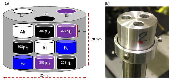
Figure 1.
(a) The cylindrical CT sample holder’s geometry, with the arrangement of the rods within the holder. (b) Picture of the CT sample during the experiment.
2.2. 3D Gamma-CT Image Measurement
Figure 2 shows a schematic diagram of the experimental setup at the beamline BL1U in the UVSOR-III facility used to measure the 3D gamma-CT image. A lead collimator with a quadrangular prism shape that was 200 mm in length, 100 mm in width, and 100 mm in height, which had a circular hole with a diameter of 1 mm, was positioned in the LCS gamma-ray beam’s path to define the diameter and the energy spectrum of the LCS gamma-ray beam on the CT sample. We operated the laser system at a typical average power of 2.4 W during measurement of the gamma-CT images to generate an LCS gamma-ray beam with an intensity of 7 × 10⁶ photons/s with 100% energy bandwidth at the full width at half maximum (FWHM) before collimation. The EGS5 Monte Carlo simulation code [19] was used to estimate the LCS gamma-ray beam’s properties after the collimation [13]. The estimated flux of the LCS gamma-ray beam after collimation was 0.7 photons/s/eV at a maximum energy of 5528 MeV with 1.1% energy bandwidth at the FWHM. Since the LCS gamma-ray beam’s divergence was small (on the order of 10−3), the diameter of the LCS beam on the CT sample was almost the same as the size of the hole in the collimator: approximately 1 mm. The flux of the incident LCS gamma-ray beam was measured using a 5-mm-thick plastic scintillator (PL) located 180 cm downstream from the collimator. After passing through the PL, the transmitted LCS gamma-ray beam was injected into the CT sample, which was installed on the three-axis traveling stage located 213 cm downstream from the collimator. The flux of the transmitted gamma rays was measured using a 3.5″ × 4″ LaBr3(Ce) scintillation detector positioned 82 cm downstream from the CT sample. This transmitted flux was used for evaluating the atomic attenuation of the sample. We chose the LaBr3(Ce) scintillation detector due to a better energy resolution, 2.7% at 662 KeV, than the NaI(Tl) scintillation detector whose typical energy resolution is approximately 6% to 8% at 662 keV. In addition, the availability of a high counting rate of the LaBr3(Ce) scintillation detector due to the short decay time is suitable for our measurement. The intrinsic radiation of the LaBr3(Ce) scintillation detector contributes significantly to the background radiation in the region below 1.6 MeV [20], which is far below our energy of interest (around 5.5 MeV). To avoid signal pile-up on the LaBr3(Ce) detector, a 5-cm-thick bismuth (Bi) absorber was placed in front of the detector. We used the bismuth as an absorber because of its high density. In addition, in the NRF-CT imaging technique, we measure the scattered NRF gamma rays from a witness target made from the isotope of interest such as the lead isotope 208Pb in our experiments. If we used lead material as an absorber, the NRF gamma rays would be contaminated by the scattered NRF gamma rays from the absorber material. Therefore, it is preferable to avoid using the isotope of interest material as an absorber. Other high-density materials, such as tungsten, can be used as absorbers as well; however, bismuth is less expensive than tungsten.
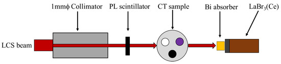
Figure 2.
Schematic diagram of the experimental setup to measure the 3D gamma-CT image at the beamline BL1U in the UVSOR-III synchrotron radiation facility.
The CT sample was scanned along three axes as follows: (i) the vertical position (y) was fixed at a set position; (ii) 2D gamma-CT images were scanned in the horizontal direction (x) across the range from −12 to +12 mm with a step size of 1 mm. The sample was scanned in each horizonal position in the direction of rotation (θ) across the range from 0 to 150 degrees with a step size of 30 degrees; (iii) (i) and (ii) were repeated for different vertical positions (y) from 1 to 22 mm with a step size of 1 mm. We gathered 3300 data points in the presence of the CT sample by measuring 25 locations along the x-axis, 22 layers in the y direction, and 6 rotational angles (θ). In addition, we measured one data point for each scan in the x direction in the absence of the CT sample. Therefore, a total of 3432 data points were measured with an average measurement time of 5 s per data point. The overall time needed to obtain the gamma-ray spectra at all data points was approximately 5 h.
2.3. 3D NRF-CT Image Measurement
We used a high-flux LCS gamma-ray beam to measure the 3D NRF-CT image. Since the total gamma-ray flux was proportional to the average power of the laser with a proportional constant of 3.5 × 10⁶ photons/s/W, we used the Tm-fiber laser system with a typical average power of 36 W to generate the LCS gamma-ray beam. When the laser system was operated at 36 W, a total flux higher than 108 photons/s with a 100% energy bandwidth could be generated. We used a collimator with a hole diameter of 2 mm, which is twice as wide as that of the collimator used for 3D gamma-CT image measurement. The LCS gamma-ray beam flux passing through the collimator was numerically estimated using the EGS5 Monte Carlo simulation code [19], and thus we found that the flux density was 10 photons/s/eV and that the maximum energy was 5528 MeV with 2.9% energy bandwidth at the FWHM, which was able to excite the Jπ = 1− NRF level at 5512 MeV in 208Pb. Although the NRF-CT imaging technique is time-consuming, we were able to shorten the image acquisition time for each measurement point, which had been measured in our previous research [13] by adjusting the CT sample scanning pattern and increasing the LCS gamma-ray beam’s intensity flux. The overall time needed to obtain a 3D NRF-CT image was approximately 48 h. Reference [14] gives more details on the experimental setup, the CT sample scanning plan, and a schematic diagram of the 3D NRF-CT image.
3. Results and Discussion
3.1. 3D-CT Primary Images
CT imaging can be performed by measuring the decrease in the gamma-ray intensity passing through a CT sample along a series of linear paths and various angles. The amount of decrease depends on the gamma-ray energy, the path lengths, and the material’s linear attenuation coefficients. Therefore, one can obtain a gamma-CT image for a sample using the gamma-ray transmission factor measurements of the off-resonance energy, known as off-resonance (εoff) attenuation, which originates from the atomic effect. The procedures of the 2D gamma-CT images calculation are detailed in references [13,14,21]. Since the height of the CT sample holder was 20 mm, we divided it into 20 layers and added two extra layers; one of the two extra layers was located below the bottom of the CT sample and the other above it. These layers were separated by a vertical distance of 1 mm. Therefore, the total number of scanned layers was 22. We assigned the labels L1 to L22 to the layers at the vertical distances of y = −1 mm to y = 21 mm, respectively. Consequently, we obtained one 2D gamma-CT image (25 × 25) with a resolution of 1 mm/pixel for each row of rods in the y direction of the CT sample scan. The pixel size was determined by the scanning step in the x direction. In total, 22 reconstructed 2D gamma-CT images were obtained, which we named to . Since Layer L1 was located beneath the CT sample holder and Layer L2 was located at the bottom edge of the holder, the LCS gamma-ray beam traveled underneath the rods. Therefore, the reconstructed images for the first two layers and did not show any characterization of the rods within the CT sample. Figure 3a shows the cross-sectional slices of the CT sample for the horizontal layers from L3 to L8. The total height of these layers was 6 mm, which was identical to the height of each rod within these layers. Two rods of enriched lead isotopes (208Pb and 206Pb) were inserted into two of the holes in the CT sample, and an Fe rod was inserted into the third hole. Figure 3b shows the reconstructed CT images from to due to the atomic attenuation measured by the LaBr3(Ce) detector. Because the lead isotope (206Pb and 208Pb) rods had the same atomic attenuation, the two high-attenuation areas in the white-colored area caused by the atomic process corresponding to the locations of these lead rods were plainly evident in all reconstructed images. However, it was difficult to discriminate between the two isotopes. Furthermore, the atomic attenuation caused by the Fe rod was smaller than that caused by the lead rods, making the Fe rod appears as a faint shadow.
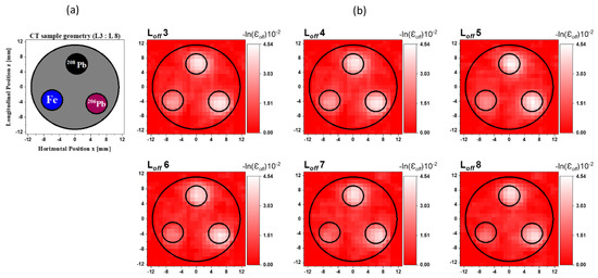
Figure 3.
(a) Cross-sectional slice images of the CT sample in the layers from L3 to L8. (b) Reconstructed images from to of the off-resonance attenuation (atomic effect) measured by the LaBr3(Ce) detector with a resolution of 1 mm/pixel.
Figure 4a shows the cross-sectional slices of the CT sample for the horizontal layers from L9 to L14. The total height of these layers was also 6 mm. Rods of 208Pb, Fe, and Al were inserted into the first, second, and third holes, respectively. The reconstructed CT images from to are shown in Figure 4b. A high-attenuation area caused by the atomic process corresponding to the 208Pb rod is clearly visible in the reconstructed images. The atomic attenuation originating from the Fe rods was less than that caused by the 208Pb rod, making the Fe rod discernible but not as apparent. Since the CT sample holder was Al, the Al rod was not visible.
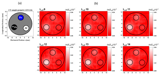
Figure 4.
(a) Cross-sectional slice images of the CT sample in the layers from L9 to L14. (b) Reconstructed CT images from to of the off-resonance attenuation (atomic effect) with a resolution of 1 mm/pixel.
The results for the horizontal layers from L15 to L20 are shown in Figure 5. Two lead isotope rods (208Pb and 206Pb) were inserted into the two holes, while the third hole remained unfilled as shown in Figure 5a. Figure 5b shows the reconstructed images from to . The two high-attenuation areas corresponding to the 206Pb and 208Pb rods can be clearly observed but they cannot be distinguished. The low-intensity area at the third hole corresponds to the vacant space.
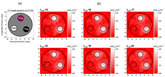
Figure 5.
(a) Cross-sectional slice images of the CT sample in the layers from L15 to L20. (b) Reconstructed CT images from to of the off-resonance attenuation (atomic effect) at a resolution of 1 mm/pixel.
Since Layers L21 and L22 were located above the inserted rods within the CT sample, the LCS gamma-ray beam did not pass through these rods. Therefore, there was no characterization for the rods in the two reconstructed images, and . The 3D-CT image was, in general, primarily made up of the 2D-CT images taken at various positions. Thus, the 22 measured 2D gamma-CT images were visualized together to create one 3D gamma-CT image. We used the MicroAVS data visualization tool [22] to create the 3D gamma-CT image with a resolution of 1 mm/pixel. Movie S1 shows the visualized 3D gamma-CT image. Figure 6 shows a shot of the 3D gamma-CT image, which was captured from the visualized 3D movie (see Movie S1 in the Supplementary Materials). We adjust a value of approximately 60% of the maximum intensity of the 2D gamma-CT images as a threshold limit for visualizing the 3D surface. Since the Fe or Al rods induced less atomic attenuation than the lead rods, this threshold limit ensured that only the lead rods appeared on the 3D surface. Intensity values greater (less) than the limit appeared (disappeared) on the 3D image. The five high-attenuation areas caused by the atomic process, which correspond to the positions of the five enriched lead isotope (208Pb and 206Pb) rods within the CT sample, are clearly visible. The gamma-CT imaging technique is capable of clearly identifying the presence of the materials to be examined. In addition, we obtained the 3D gamma-CT image with a higher resolution and shorter acquisition time than the NRF-CT imaging technique. However, it lacked the isotope-selective capability needed to distinguish between different isotopes of the same element. Therefore, we utilized the 3D gamma-CT image as an additional information source to improve the quality of the 3D isotope-selective CT imaging based on the NRF transmission method.
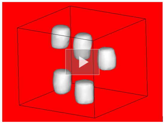
Figure 6.
A shot of the three-dimensional visualization of the atomic attenuation (3D gamma-CT image). See coresponding Movie S1 in the Supplementary Materials.
For the primary 3D NRF-CT image, we chose the layers at the vertical distances of z = 3, 11, and 17 mm, measured from the holder’s bottom, to reconstruct the 2D NRF-CT images of , , and , respectively. One 2D NRF-CT (7 × 7) image was obtained for each horizontal row of rods (see Figure 1a). In our previous study [14], we reported the visualization of the reconstructed 3D images with a resolution of 4 or 8 mm/pixel for the horizontal or vertical plane, respectively, which were based on the atomic attenuation and the pure NRF attenuation. The measurement procedure, numerical equations, and 2D NRF-CT images were reported in [14]. If a 3D NRF-CT image were measured under the current gamma-ray flux and detection efficiency available at the BL1U in the UVSOR-III facility, the total required time for obtaining a 3D NRF-CT with a spatial resolution of 1 mm is expected to be 2640 h. Thus, we need an alternative method to improve the resolution of the 3D NRF-CT image without needing a long measurement time. We used an FV numerical treatment to obtain a higher-quality image with a resolution of 1 mm/pixel with a measuring time shorter than that required to get the desired resolution without this treatment. In the following sub-section, we detail the FV approach.
3.2. Post-Multiply FV Method
One of the FV numerical approaches is the so-called “post-multiply FV method”, which analyzes a 3D gamma-CT image with a resolution of 1 mm/pixel as an additional data source to improve the resolution of the 3D NRF-CT image [14]. The procedure of the post-multiply FV method is as follows: (i) sinogram adjustment, (ii) layer alignment (x, θ), (iii) 2D gamma-CT image segmentation, (iv) 2D-CT image overlapping, and (v) image visualization in 3D.
- (I)
- Sinogram Adjustment
The transmission factors of the off-resonance attenuation (εoff) and the on-resonance attenuation (εNRF) [14] were gathered into a 2D matrix (sinogram). The size of the two-dimensional sonogram was determined by the scanning steps in the x direction and the θ angle. We obtained the 2D gamma-CT images by scanning the CT sample in the x direction with a 1 mm step size across the range from −12 to +12 (25 positions). Furthermore, we scanned the CT sample in the θ direction with an angle step of 30° across the range from 0° to 150° (six angles). Therefore, we obtained sinograms of the εoff transmission factor in a matrix with a size of 25 × 6. Moreover, the reconstructed 2D gamma-CT images had a matrix size of 25 × 25. For the 2D NRF-CT images, we scanned the CT sample in the x direction with a 4 mm step size across the range from −12 to +12 (seven positions). We scanned the CT sample in the θ direction with an angle step of 30° across the range from 0° to 150° (six angles). Therefore, we obtained sinograms of the ԐNRF transmission factor with a size of 7 × 6 [14]. The reconstructed 2D NRF-CT images had a matrix size of 7 × 7. For overlapping the two 2D-CT images resulting from the sinograms of the reconstructed transmission factors ԐNRF and Ԑoff, the images needed to have the same size in both directions (x and z). In order to ensure the two images had the same size in both directions, we introduced a sinogram adjustment process to numerically divide each ԐNRF sinogram from with a dimension of 7 × 6 to with a dimension of 25 × 6 as follows: we divided each value in the x direction equally into 25 values to create a sinogram (x, θ) with a dimension of 175, 6. We then combined each seven consecutive values together into one value to create a new sinogram in a dimension of 25 × 6. Therefore, the newly reconstructed images had a size of 25 × 25.
- (II)
- Layer Alignment (x, θ)
We measured the 22 layers of the gamma-CT measurement ( to ) in addition to the three layers of the NRF-CT measurement (), and we aligned every image to a group with six 2D gamma-CT images measured for six consecutive layers. Figure 7 illustrates the aligned layers in the vertical direction for both kinds of images. We aligned the 2D gamma-CT images from to , which included the rods of 208Pb, 206Pb and Fe, with the image of . We also aligned the 2D gamma-CT images from to , which included the rods of 208Pb, Fe, and Al, with the image of . The 2D gamma-CT images from to , including the 206Pb and 208Pb rods in addition to the vacant area, were aligned with the image of .
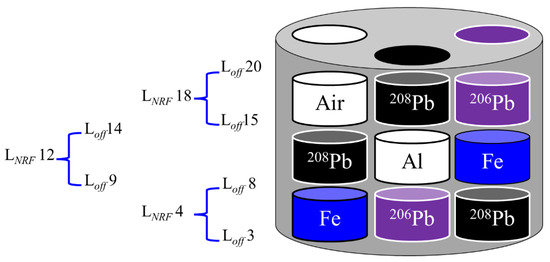
Figure 7.
The arrangement of the inserted rods within the CT sample holder and the scanned layers in the z direction used for the 2D gamma-CT and NRF-CT images.
- (III)
- 2D Gamma-CT Image Segmentation
Image segmentation is a process of partitioning an image into numerous segments or a process of placing pixels such that they have non-overlapping areas [23]. This segmentation procedure is the first stage of image analysis [24], object representation, visualization, and other image processing strategies used in a variety of fields [25]. The main goal of image segmentation is to simplify and/or transform an image into one that can be readily analyzed [24]. In the case of segmentation of a 2D gamma-CT image, we assumed that the atomic absorption intensities varied in some regions of the CT sample and that the intensity at each pixel in a region where a rod existed would be almost constant. The first step of 2D gamma-CT image segmentation was primary image scaling. We scaled the primary gamma-CT images to a value between 0 and 255. The range of 0 to 255 was chosen to provide for an 8-bit representation of each pixel. The black, gray, and white colors were represented by values of 0, 128, and 255, respectively. One of the most commonly used approaches used for image segmentation is the threshold method [24,26]. Thresholding plays a crucial role in various algorithms used for image analysis, object representation, and visualization [27]. In this method, we chose a threshold value (Tr) for transforming an image from a grayscale into a binary image, in which each pixel has a value of 0 or 1, to distinguish the foreground and background of the image [28]. A pixel with an intensity greater (lower) than Tr is shown by a white-colored (black-colored) area. Threshold methods are grouped into two types: local thresholding and global thresholding. The local thresholding methods apply different threshold values to different regions of the image. Each Tr value is determined by the neighborhood of the pixel to which the threshold is applied [26,29]. On the other hand, in global thresholding, a single Tr value is used to separate the foreground and the background for all pixels in an image [24,30]. In the present analysis, we performed global thresholding with a common threshold Tr value of 128 as the second step of gamma-CT image segmentation. The black and white 2D segmented gamma-CT images of the scanned layers are shown in Figure 8, with the layers labeled from to . The positions of the inserted rod turned entirely white, while the residual areas turned black. The image segmentation procedure resulted in a set of segments that collectively covered the whole image or a set of contours as the object’s edge. Each pixel in the inserted rods’ positions had a common property such as color or intensity. Furthermore, the neighboring areas differed substantially in terms of the same characteristic. When 2D segmented gamma-CT images are created for the employment of the FV technique with the NRF-CT images after the gamma-CT image segmentation, the resulting contours can be used to precisely preserve the 208Pb rod locations within the gamma-ray images of the CT sample and cut the surrounding noise and distortions.
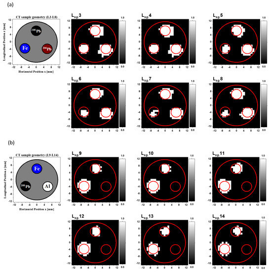
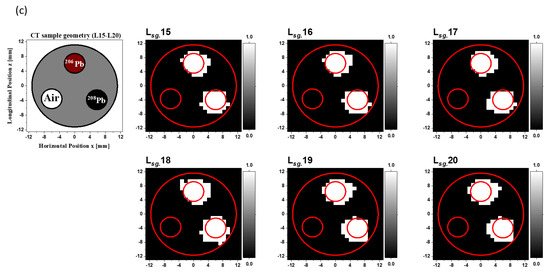
Figure 8.
(a–c). Cross-sectional slice images of the CT sample in the layers from L3 to L20, in addition to the binary (0,1) 2D Tr gamma-CT images.
- (IV)
- 2D-CT Image Overlapping
We overlapped the primary 2D-CT images to obtain a 2D FV NRF-CT image as follows: the images of Layers , , and were overlapped with the 2D segmented gamma-CT images from to , to , and to , respectively, according to the following equation:
We labeled the resulting 2D FV NRF-CT images as to . While the 208Pb rod is clearly visible in the fused images from to , as shown in Figure 9a, the Fe and 206Pb rods are almost invisible. Figure 9b shows the fused images from to . Only the 208Pb rod can be seen clearly, but neither the Fe nor the Al rods are visible. Moreover, we can clearly pinpoint the location of the 208Pb rod in the reconstructed images from to , as shown in Figure 9c. The 206Pb rod and the vacant area disappeared. Obviously, the noise in all 2D FV NRF-CT image backgrounds caused by using the post-multiply FV method for the primary data sources was totally eliminated from the reconstructed image background. Since the overlapping process of the post-multiply FV method was performed by multiplying the intensity value at each pixel in the by a value of 1 within the 208Pb locations or by a value of 0 in the surrounding regions, the method preserved the locations of the isotopes of interest and completely eliminated the surrounding distortion and background noise. Furthermore, it kept the intensity value at each pixel constant, making this approach useful for isotope quantification.
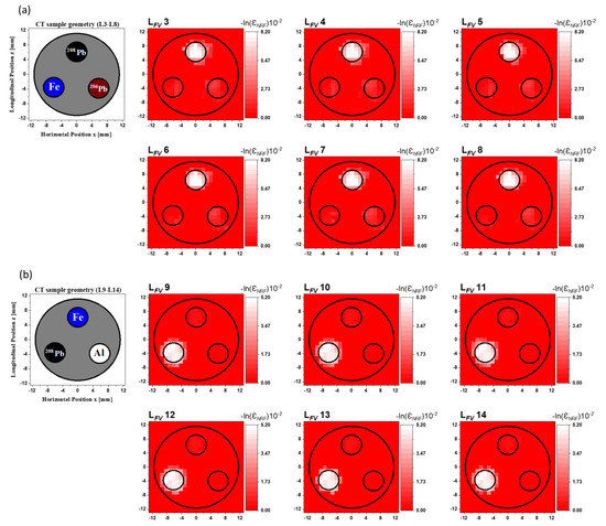
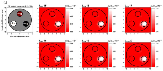
Figure 9.
Reconstructed 2D FV NRF-CT images from (a) to , (b) to , and (c) to for the post-multiply FV method with the CT sample’s geometry for each layer group.
- (V)
- Image Visualization in 3D
The 22 2D FV NRF-CT images were combined together using the MicroAVS data visualization tool to create the 3D FV NRF-CT image. We also adjusted a value within the intensity range of the 2D FV NRF-CT images as a threshold limit, so that only the intensity values greater than the threshold limit (208Pb rods) appeared on the 3D surface. Movie S2 shows a visualization of the fused CT-image of the NRF attenuation caused by the 208Pb isotope rods within the CT sample (pure NRF) in three dimensions. Figure 10 shows a shot of the 3D FV NRF-CT image, which was captured from the visual-ized 3D movie (see Movie S2 in the Supplementary Materials). The visualization clearly shows the locations of the enriched lead isotope (208Pb) rods. In contrast, the rods of 206Pb, Fe, and Al and the empty areas are not visible.
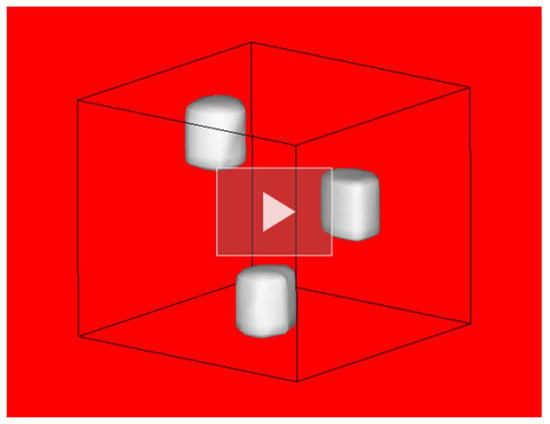
Figure 10.
A shot of the three-dimensional visualization of the fused CT-image of the NRF attenuation caused by the distribution of 208Pb (3D FV NRF-CT image). See corresponding Movie S2 in the Supplementary Materials.
We obtained an isotope-selective 3D FV NRF-CT image with a resolution of 1 mm/pixel for the distribution of an enriched lead isotope (208Pb) inserted with rods of different materials within a cylindrical sample 20 mm in height and 25 mm in diameter. Since the fused image has the same pixel resolution as the primary gamma-CT image, the image distortion and the background noise vanished, and the locations of the 208Pb rods were clearly visible. In contrast, the other rods completely disappeared, since their intensity values were less than the selected threshold limit of the 3D surface. Therefore, the combination of primary 3D NRF-CT images with high-resolution 3D gamma-CT images obtained by the FV technique provided a beneficial improvement in the image resolution and the isotope-selective capability in three dimensions.
The numerical treatment of the FV technique can be used in different approaches for primary 3D-CT images. Most of these approaches are similar to the post-multiply FV method, except for a few minor differences. One of the approaches is to directly overlap a 2D NRF-CT image with a 2D gamma-CT image without the 2D gamma-CT image segmentation process according to the following equation:
The 2D FV NRF-CT image obtained by this approach in the current study had the required quality. However, it could not be used for isotope quantification because the intensity at each pixel of the NRF-CT image was not conserved. Furthermore, even if the background noise were significantly reduced, it would be impossible to eliminate all noise. Another approach is the post-sum FV method, for which the overlapping is as follows:
The fused image obtained using the post-sum FV method shows the change in the intensity at each pixel but retains some of the background noise, so this method is useless for isotope quantification. Figure 11 shows a comparison between the 2D FV NRF-CT images for the layer L4 obtained by (a) the post-multiply FV method, (b) the post-multiply FV method without 2D gamma-CT image segmentation, and (c) the post-sum FV method.
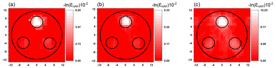
Figure 11.
(a) 2D NRF-CT images obtained via the post-multiply FV method, (b) the post-multiply FV method (without 2D gamma-CT image segmentation), and (c) the post-sum FV method for layer L4.
These results show that the alternative approaches may change the intensity of each pixel, so that they are unable to maintain the quantity of the isotope of interest. Furthermore, the noise cannot be completely removed even if it can be greatly decreased. Therefore, we recommend the post-multiply FV method as the most beneficial method for NRF-CT imaging that is likely to be effectively applicable in a variety of fields, including nuclear engineering and nuclear safety.
4. Conclusions
The fusion visualization (FV) technique can be used as an effective numerical treatment to improve computed tomography (CT) imaging based on the nuclear resonance fluorescence (NRF) transmission method. We obtained two three-dimensional (3D) CT images for the distribution of an enriched lead isotope (208Pb) inserted into a cylindrical holder together with rods of various materials (another enriched lead isotope of 206Pb, iron, and aluminum). One of the images was the isotope-selective 3D CT image based on the NRF transmission method, which had a relatively low resolution. The other was a significantly higher-resolution 3D gamma-CT image. The two images were measured at the beamline BL1U in the ultraviolet synchrotron orbital radiation-III (UVSOR-III) synchrotron radiation facility at the Institute of Molecular Science at the National Institutes of Natural Sciences in Japan. We generated a laser Compton scattering (LCS) gamma-ray beam with a maximum energy of 5528 MeV, which was able to excite the Jπ = 1− state at 5512 MeV in 208Pb. We used two LCS beams with different intensities and beam diameters for two experiments. First, we generated an LCS gamma-ray beam with a diameter of 1 mm and a flux of 0.7 photons/s/eV to obtain a 3D gamma-CT image with a resolution of 1 mm/pixel. Next, we generated an LCS gamma-ray beam with a diameter of 2 mm and a flux of 10 photons/s/eV to measure the 3D NRF-CT image with a resolution of 4 and 8 mm/pixel in the horizontal and vertical planes, respectively. We applied the FV technique using the post-multiply FV method between the two primary images to create a 3D isotope-selective fused CT image based on the NRF transmission method (3D FV NRF-CT) for the distribution of 208Pb in the CT sample. The background noise in the fused 3D image was removed and the quantity of the isotope of interest was conserved. Although we also examined the direct overlapping method and the post-sum FV method, we concluded that the post-multiply FV method was the most suitable for isotope-selective CT imaging to be used in nuclear engineering and various nuclear applications.
Supplementary Materials
The following are available online at https://www.mdpi.com/article/10.3390/app112411866/s1, Movie S1: Three-dimensional visualization of the atomic attenuation (3D gamma-CT image), Movie S2: Three-dimensional visualization of the fused CT image of the NRF attenuation caused by the distribution of 208Pb (3D FV NRF-CT image).
Author Contributions
Conceptualization, H.O.; data curation, K.A. and H.Z.; formal analysis, K.A.; funding acquisition, H.O., T.H. and T.S.; investigation, K.A., H.O. and H.Z.; methodology, K.A., H.Z., H.O., T.H. and T.S.; project administration, H.O.; resources, H.O., T.H., T.S. and M.K.; software, K.A. and H.Z.; supervision, H.O.; validation, K.A., H.Z., H.O., T.K., T.H., T.S., M.K., Y.T., M.F. and H.T.; visualization, K.A., H.Z. and H.O.; writing—original draft, K.A.; writing—review and editing, K.A., H.Z., H.O., T.K., T.H., T.S., M.K., Y.T., M.F. and H.T. All authors have read and agreed to the published version of the manuscript.
Funding
This research was funded by the Japan Society for the Promotion of Science (JSPS) KAKENHI under Grants 18H01916, 18H03715, and 17K05482.
Informed Consent Statement
Not applicable.
Acknowledgments
This work was performed at the beamline BL1U of the UVSOR-III Synchrotron Radiation Facility with the approval of the Institute for Molecular Science (IMS), National Institute of Natural Science (NINS), Okazaki 444-8585, Japan (Proposal No. 19-503 and 20-703).
Conflicts of Interest
The authors declare no conflict of interest. The funders had no role in the design of the study; in the collection, analyses, or interpretation of data; in the writing of the manuscript; or in the decision to publish the results.
References
- Metzger, F. Resonance fluorescence in nuclei. Progr. Nucl. Phys. 1959, 7, 54–88. [Google Scholar]
- Bertozzi, W.; Ledoux, R.J. Nuclear resonance fluorescence imaging in non-intrusive cargo inspection. Nucl. Instrum. Methods Phys. Res. Sect. B Beam Interact. Mater. At. 2005, 241, 820–825. [Google Scholar] [CrossRef]
- Pruet, J.; McNabb, D.P.; Hagmann, C.A.; Hartemann, F.V.; Barty, C.P.J. Detecting clandestine material with nuclear resonance fluorescence. J. Appl. Phys. 2006, 99, 123102. [Google Scholar] [CrossRef]
- Hajima, R.; Hayakawa, T.; Kikuzawa, N.; Minehara, E. Proposal of nondestructive radionuclide assay using a high-flux gamma-ray source and nuclear resonance fluorescence. J. Nucl. Sci. Technol. 2008, 45, 441–451. [Google Scholar] [CrossRef]
- Kikuzawa, N.; Hajima, R.; Nishimori, N.; Minehara, E.; Hayakawa, T.; Shizuma, T.; Toyokawa, H.; Ohgaki, H. Nondestructive detection of heavily shielded materials by using nuclear resonance fluorescence with a laser-Compton scattering γ-ray source. Appl. Phys. Express 2009, 2, 036502. [Google Scholar] [CrossRef]
- Hayakawa, T.; Kikuzawa, N.; Hajima, R.; Shizuma, T.; Nishimori, N.; Fujiwara, M.; Seya, M. Nondestructive assay of plutonium and minor actinide in spent fuel using nuclear resonance fluorescence with laser Compton scattering γ-rays. Nucl. Instrum. Methods Phys. Res. Sect. A Accel. Spectrom. Detect. Assoc. Equip. 2010, 621, 695–700. [Google Scholar] [CrossRef]
- Quiter, B.J.; Ludewigt, B.A.; Mozin, V.V.; Wilson, C.; Korbly, S. Transmission nuclear resonance fluorescence measurements of 238U in thick targets. Nucl. Instrum. Methods Phys. Res. Sect. B Beam Interact. Mater. At. 2011, 269, 1130–1139. [Google Scholar] [CrossRef]
- Arutyunian, F.R.; Tumanian, V.A. The Compton effect on relativistic electrons and the possibility of obtaining high energy beams. Phys. Lett. 1963, 4, 176–178. [Google Scholar] [CrossRef]
- Milburn, R.H. Electron scattering by an intense polarized photon field. Phys. Rev. Lett. 1963, 10, 75–77. [Google Scholar] [CrossRef]
- Barty, C.P.; Albert, F.; Anderson, S.G.; Armstrong, P.; Bayramian, A.; Beer, G.; Cross, R.; Ebbers, C.A.; Deis, G.; Gibson, D.J.; et al. Overview of MEGa-Ray-Based Nuclear Materials Management Activities at the Lawrence Livermore National Laboratory; Institute of Nuclear Materials Management: Palm Desert, CA, USA, 2011. [Google Scholar]
- Bertozzi, W.; Ledoux, R.J. Methods and Systemic For Computer Tomography of Nuclear Isotopes Using Nuclear Resonance Fluorescence. U.S. Patent 8,180,019 B2, 15 May 2012. [Google Scholar]
- Zen, H.; Ohgaki, H.; Taira, Y.; Hayakawa, T.; Shizuma, T.; Daito, I.; Yamazaki, J.-i.; Kii, T.; Toyokawa, H.; Katoh, M. Demonstration of tomographic imaging of isotope distribution by nuclear resonance fluorescence. AIP Adv. 2019, 9, 035101. [Google Scholar] [CrossRef]
- Ali, K.; Ohgaki, H.; Zen, H.; Kii, T.; Hayakawa, T.; Shizuma, T.; Toyokawa, H.; Taira, Y.; Iancu, V.; Turturica, G.; et al. Selective isotope CT imaging based on nuclear resonance fluorescence transmission method. IEEE Trans. Nucl. Sci. 2020, 67, 1976–1984. [Google Scholar] [CrossRef]
- Ali, K.; Ohgaki, H.; Zen, H.; Kii, T.; Hayakawa, T.; Shizuma, T.; Toyokawa, H.; Taira, Y.; Fujimoto, M.; Katoh, M. Three-dimensional nondestructive isotope-selective tomographic imaging of 208Pb distribution via nuclear resonance fluorescence. Appl. Sci. 2021, 11, 3415. [Google Scholar] [CrossRef]
- Ziock, K. Principles and applications of gamma-ray imaging for arms control. Nucl. Instrum. Methods Phys. Res. Sect. A Accel. Spectrom. Detect. Assoc. Equip. 2018, 878, 191–199. [Google Scholar] [CrossRef]
- Diaz, J.; Kim, T.; Petrov, V.; Manera, A. X-ray and gamma-ray tomographic imaging of fuel relocation inside sodium fast reactor test assemblies during severe accidents. J. Nucl. Mater. 2021, 543, 152567. [Google Scholar] [CrossRef]
- Wahl, C.G.; Kaye, W.R.; Wang, W.; Zhang, F.; Jaworski, J.M.; King, A.; Boucher, Y.A.; He, Z. The Polaris-H imaging spectrometer. Nucl. Instrum. Methods Phys. Res. Sect. A Accel. Spectrom. Detect. Assoc. Equip. 2015, 784, 377–381. [Google Scholar] [CrossRef]
- Duc, T.P.; Nakamura, R. Fused visualization of 3D Ultrasound and CT image on navigation system for water-filled laparo-endoscopic surgery. Trans. Jpn. Soc. Med. Biol. Eng. 2014, 52, O-303–O-304. [Google Scholar]
- Hirayama, H.; Namito, Y.; Bielajew, A.F.; Wilderman, S.J.; Nelson, W.R. The EGS5 Code System; SLAC-R-730 (2005) and KEK Report Number: 2005-8; Department of Energy: Washington, DC, USA, 2009.
- Sangang, L.; Yi, C.; Lei, W.; Li, Y.; Huan, L.; Jiawei, L.; Liyang, Z.; Yong, L.; Xiaoyu, W.; Qiuyan, P.; et al. The Effect of Intrinsic Radiation from a 3 × 3-in. LaBr3(Ce) Scintillation Detector on In Situ Artificial Radiation Measurements. Nucl. Tech. 2018, 204, 195–202. [Google Scholar] [CrossRef]
- Daito, I.; Ohgaki, H.; Suliman, G.; Iancu, V.; Ur, C.A.; Iovea, M. Simulation study on computer tomography imaging of nuclear distribution by quasi monoenergetic gamma rays with nuclear resonance fluorescence: Case study for ELI-NP application. Energy Procedia 2016, 89, 389–394. [Google Scholar] [CrossRef]
- AVS. General Purpose Visualization Software. Cybernet Systems Co., Ltd. Available online: https://www.cybernet.co.jp/avs/sitemap.html (accessed on 1 April 2021).
- Tavares, J.M.R.; Natal, J.R. Computational Vision and Medical Image Processing IV, 1st ed.; CRC Press: London, UK, 2013; p. 492. [Google Scholar]
- Shapiro, L.G.; Stockman, G.C. Computer Vision; illustrated ed.; Prentice Hall: Hoboken, NJ, USA, 2001; pp. 97–106. [Google Scholar]
- Evelin, S.G.; Lakshmi, Y.V.S.; Jiji, G.W. MRI brain image segmentation based on thresholding. Int. J. Adv. Comput. Res. 2013, 3, 97–101. [Google Scholar]
- Senthilkumaran, N.; Vaithegi, S. Image segmentation by using thresholding techniques for medical images. Comput. Sci. Eng. Int. J. 2016, 6, 1–13. [Google Scholar]
- Goh, T.Y.; Basah, S.N.; Yazid, H.; Safar, M.J.A.; Saad, F.S.A. Performance analysis of image thresholding: Otsu technique. Measurement 2018, 114, 298–307. [Google Scholar] [CrossRef]
- Huang, K.; Wang, L.; Mao-Jiun, J. Image thresholding by minimizing the measures of fuzziness. Pattern Recognit. 1995, 28, 141–151. [Google Scholar] [CrossRef]
- Devi, H. Thresholding: A Pixel-level image processing methodology preprocessing technique for an OCR system for the Brahmi script. Anc. Asia 2006, 1, 161–165. [Google Scholar] [CrossRef][Green Version]
- Otsu, N. A Threshold selection method from gray-level histograms. IEEE Trans. Syst. Man Cybern. 1979, 9, 62–66. [Google Scholar] [CrossRef]
Publisher’s Note: MDPI stays neutral with regard to jurisdictional claims in published maps and institutional affiliations. |
© 2021 by the authors. Licensee MDPI, Basel, Switzerland. This article is an open access article distributed under the terms and conditions of the Creative Commons Attribution (CC BY) license (https://creativecommons.org/licenses/by/4.0/).