Using Feedback Strategies in Simulated Annealing with Crystallization Heuristic and Applications

Abstract

This paper represents how typical advanced engineering design can be structured using a set of parameters and objective functions corresponding to the nature of the problem. The set of parameters can be in different types, including integer, real, cyclic, combinatorial, interval, etc. Similarly, the objective function can be presented in various types including integer (discrete), float, and interval. The simulated annealing with crystallization heuristic can deal with all these combinations of parameters and objective functions when the crystallization heuristic presents a sensibility for real parameters. Herein, simulated annealing with the crystallization heuristic is enhanced by combining Bates and Gaussian distributions and by incorporating feedback strategies to emphasize exploration or refinement, or a combination of the two. The problems that are studied include solving an electrical impedance tomography problem with float parameters and a partially evaluated objective function represented by an interval requiring the solution of 32 sparse linear systems defined by the finite element method, as well as an airplane design problem with several parameters and constraints used to reduce the explored domain. The combination of the proposed feedback strategies and simulated annealing with the crystallization heuristic is compared with existing simulated annealing algorithms and their benchmark results are shown. The enhanced simulated annealing approach proposed herein showed better results for the majority of the studied cases.

1. Introduction

The solution of engineering problems often involves optimization. There are several well-known optimization methods, mainly based on the cost function gradient property. These methods require a seed to start the search and perform the search walking in the direction of the largest gradient [1]. However, in many applications, these methods cannot be used. The difficulties are that either the gradient property is not available, the gradient property is noisy, or the cost function is discrete. These methods are called deterministic methods because, starting from a given seed, the final result is always the same. The determination of the seed is also an additional task which eventually cannot be easily determined.

To overcome problems such as the gradient property of the cost function and seed determination, a large set of metaheuristic methods have been proposed. Usually, metaheuristics mimic some emergent behavior from nature. Genetic Algorithms (GA) [2] model the dominance of stronger creatures over weaker creatures. GA has two conventional operators: crossover and mutation. Particle Swarm Optimization (PSO) [3] models the learning task, where creatures can learn from themselves or from others. Simulated annealing (SA) [4] is a stochastic metaheuristic which models metal annealing. Differential Evolution [5] tries to improve upon a current solution given a measure of quality. Several other metaheuristics have been proposed, each of them having a specific motivation, usually from nature.

The metaheuristics do not need a seed, and they do not use any gradient property of cost functions. They are connected with the types of parameters and the cost function. For example, GA originally manipulated integer or limited precision parameters. Modifications in the original GA, such as increasing the number of operators, allow its usage even in combinatorial problems [6]. The PSO was originally proposed to deal with real parameters, and modifications in the original approach also allow its application to combinatorial problems [7].

Combinatorial problems are considered the most difficult type of problem—they are called NP-hard problems. SA was originally proposed to deal with combinatorial problems, such as traveling salesman and graph partitioning problems. It is the only metaheuristic that has a proof of convergence to the global optimum [8]. SA is the simplest algorithm with only two loops. However, it has been difficult to include real parameters in the SA. This paper explains the motivations towards the enhancement of SA to manipulate real parameters and the proposed SA with the crystallization heuristic. The crystallization heuristic does not interfere with combinatorial or integer parameters. SA with the crystallization heuristic uses feedback to control the parameter named the crystallization factor, which represents the parameter sensibility [9]. SA with the crystallization heuristic was successfully applied to problems with discrete cost functions [10,11,12]. This research improves the crystallization heuristic by combining the Bates and Gaussian distributions. Additionally, feedback strategies are proposed to emphasize the desired behavior through exploration or refinement. This proposal improves upon the results of the benchmark test from the literature.

This paper starts by explaining the proposed SA with the crystallization heuristic. Section 2 also describes several proposals for the use of real parameters with SA and the motivation to propose SA with the crystallization heuristic. Section 3 presents the results of solving some benchmark problems with SA with the crystallization heuristic. Section 4 describes an extension of SA with the crystallization heuristic in which the cost function is partially evaluated. This is called interval SA with the crystallization heuristic. The study case solves the electrical impedance tomography problem. Section 5 explains that the crystallization factor is related to the parameter sensibility. This is an important property which can enhance the SA convergence. The study case solves the airplane design problem, which is a constrained problem. All study cases are related to design and manufacturing problems. Finally, Section 6 presents the conclusions.

2. SA with Crystallization Heuristic and Feedback Strategies

SA is a popular nature-based optimization technique, and it shares many features with other meta-heuristics. Although the final solution is not guaranteed to be optimal, SA can be applied to a wide range of problems (different types of variables and objective functions) and is capable of escaping local optima when searching for a solution.

The SA algorithm was inspired by a mathematical simulation of atoms in equilibrium at a given temperature [13]. The algorithm was subsequently formalized by [14], incorporating the atom equilibrium configuration simulation by using a multivariate combinatorial optimizer. In [15], the algorithm was later extended for use with continuous variables.

At its core, SA is an iterative method with the so-called temperature parameter decreasing during execution and influencing the solution selection process. In a typical SA application, the solution is modified at each iteration, defining a candidate, and the objective function is reevaluated. If the candidate cost is smaller, then the modification is accepted. If the new cost is larger, then the modification is accepted with the probability

$$P(\Delta E)=exp(-\Delta E/T)$$

(1)

where $\Delta E$ is the difference between the current and previous costs, k is the Boltzman constant, and T is the current temperature.

This procedure allows the search to escape local optima, with the temperature parameter influencing how likely a worse solution is to be accepted; at higher temperatures, a worse solution is more likely to be accepted, whereas the inverse is true for lower temperatures. Therefore, the control of the temperature parameter, defined by the cooling schedule, has a significant impact on the effectiveness of the SA algorithm.

Algorithm 1 shows the pseudo code of a basic implementation of the SA algorithm. The algorithm consists of two nested loops: the external loop controls the temperature and the internal loop performs the solution modifications.

Algorithm 1 Basic SA

$x\leftarrow <$ random initial solution > $T\leftarrow <$ initial temperature $T_0>$ while < The global condition is not satisfied> do   while < The local condition is not satisfied> do     $x^{*}\leftarrow <$ modified solution >     $\Delta E=F\left(x^{*}\right)-F\left(x\right)$     if $\Delta E<0$ then      $x\leftarrow x^{*}$    else if $\mathrm{random}(0,1)<exp(-\Delta E/T)$ then      $x\leftarrow x^{*}$    end if   end while   $T\leftarrow T\ast \alpha$ end while

Parameter $\alpha$ controls the cooling schedule within the external loop. During each iteration of the inner loop, a new solution $x^{*}$ is created by modifying $x$, the new cost is evaluated, and the modification is either accepted or rejected. The local condition that controls the inner loop can be a fixed number of iterations or accepted candidates. On the other hand, the global stop condition is more application-specific, but usually reflects the solution convergence.

2.1. How to Modify the Solution with Continuous Variables

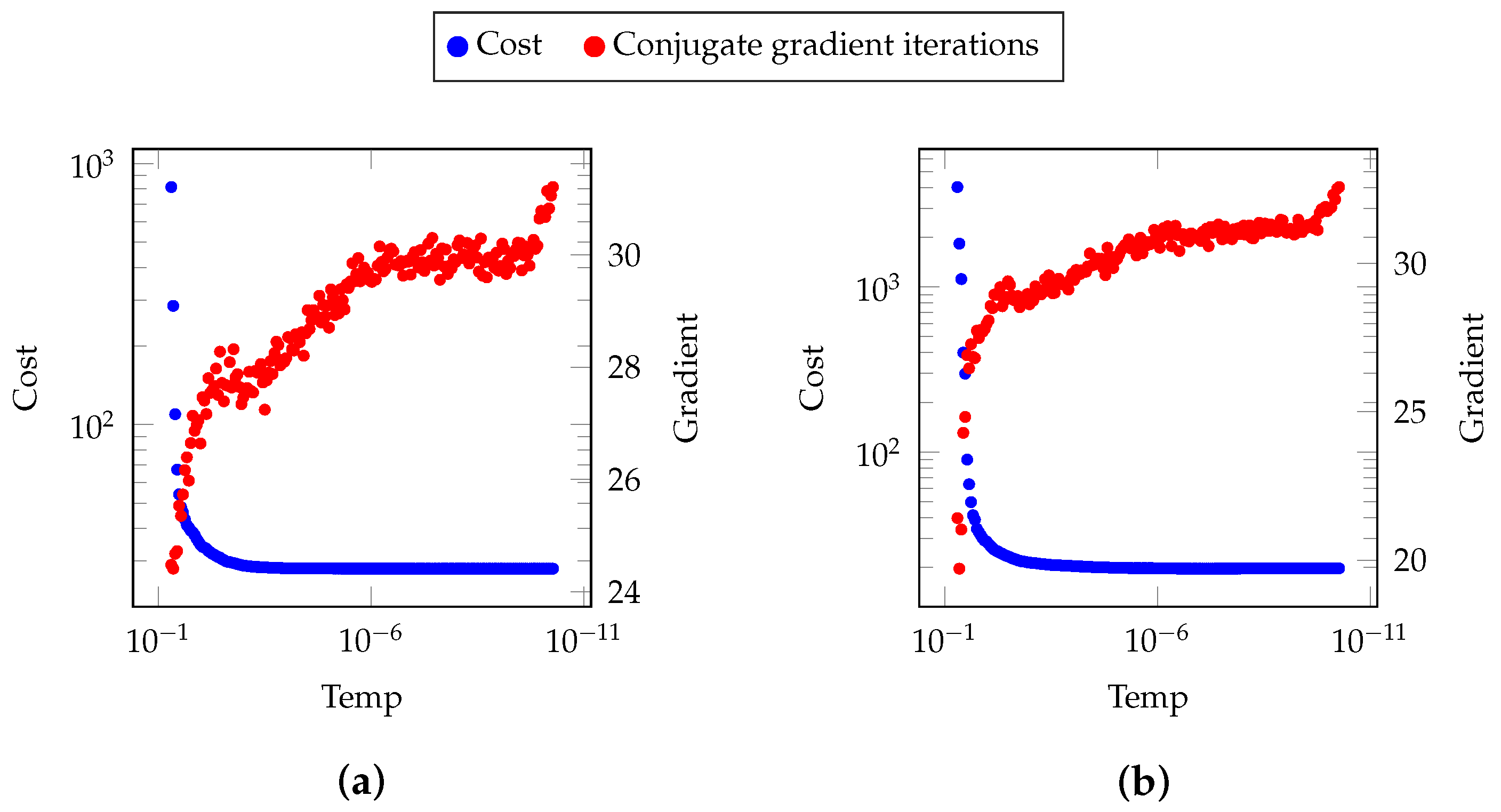
An important part of the algorithm is the generation of $x^{*}$. Several different strategies can be used to determine a new candidate during the random search step in the SA algorithm. The original SA proposed by Kirkpatrick et al. [14] was applied to the traveling salesman problem, which is a combinatorial problem. In this case, $x^{*}$ is just a permutation of $x$. They showed that SA clearly has two phases. At higher temperatures, SA explores the domain, and at lower temperatures, SA refines the solution.

Bohachevsky et al. [16] presented one of the first proposals to approach continuous problems using SA. They determined the next candidate $x^{*}$ by combining a random $\parallel \mathit{u}\parallel =1$ and a fixed step size $\Delta r$, as 

$$x^{*}=x+\Delta r·\mathit{u}.$$

When a fixed step size is considered, SA always stays in the same phase of exploration or refinement. Usually, larger steps are associated with the exploratory phase, and smaller steps are associated with the refinement phase. Bohachevsky et al. proposed that the step size $\Delta r$ must consider the objective function derivative information. If the objective function derivative related to a specific parameter i is large, this specific parameter step size $\Delta r_i$ must be small. The same reasoning works in the opposite direction. Besides the connection with the derivative information, each parameter must have its own specific step size. The connection with the derivative information proposed by Bohachevsky et al. is a weak point.

Corana et al. [15] used another important concept: the number of accepted candidates must be increased, but the number of accepted candidates must not be extremely high. For higher temperatures, the SA can accept bad candidates with higher probabilities, as can be seen from (1). If the percentage of accepted candidates is $100\%$, the search is completely aleatory. It is necessary to have a balance between accepted and rejected candidates. Corana et al. proposed that the step size must be defined in such a way that the balance between accepted and rejected candidates is kept. This proposal was good, as the relation with the derivative information was removed. Ingber et al. [17] realized that if the step size is too small, SA cannot escape from some local minimum. Thus, the step size must be kept large enough, and despite the step size always being the same, each variable has its probability distribution. Bohachevsky et al. [16] and Corana et al. [15] adopted a fixed constant probability distribution for each variable. Ingber proposed that the standard deviation of the probability distribution is related to the objective function derivative.

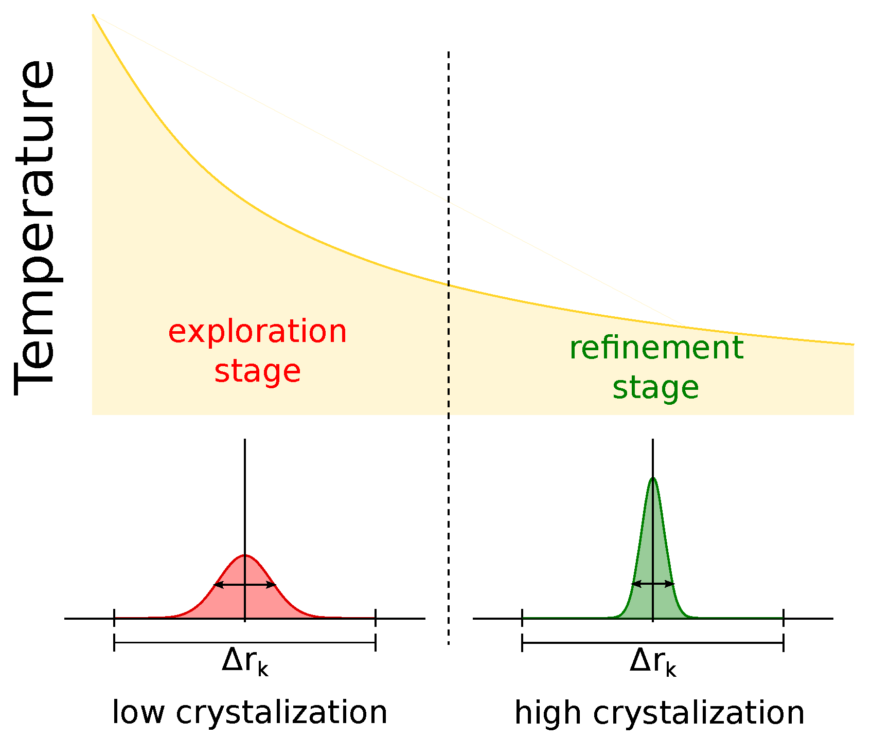
Martins and Tsuzuk [10,18] understood that the relation between the standard deviation and objective function derivative is not good. They proposed a feedback control method which keeps the number of accepted candidates at a reasonable level. The control variable is called the crystallization factor, and it represents the standard deviation of the probability distribution. Figure 1 shows the two phases of SA: exploration and refinement [19]. Associated with the phase, the probability distribution standard deviation is also represented. The standard deviation must be larger at higher temperatures and will allow larger jumps at higher temperatures. At lower temperatures, the behavior is exactly the opposite, where smaller jumps will have a higher probability of happening.

Considering a specific k-th variable represented by $e_k$, a vector with all elements zero and just the k-th element equal to 1 is created. This variable has step size $\Delta r_k$ and crystallization factor $c_k$. The next candidate is determined by

$$x^{*}=x+\frac{1}{c_k}\left[\sum _{i=1}^{c_k}\mathrm{random}(-1,+1)\right]·\Delta r_k·e_k.$$

(2)

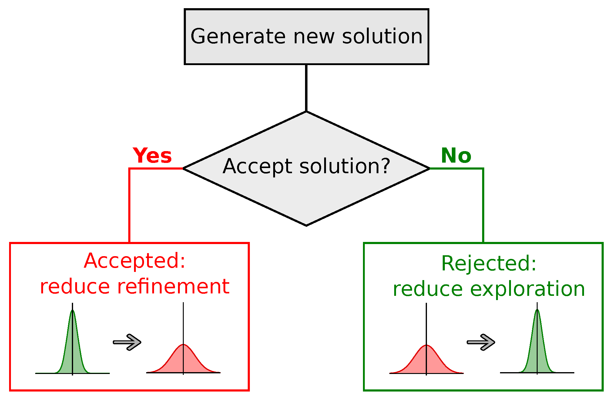
The summation of random numbers creates a Bates distribution [20] defined by the crystallization factor $c_k$. The crystallization factor is controlled by a feedback mechanism shown in Figure 2. If the candidate is accepted, the crystallization factor $c_k$ is reduced and, consequently, the standard deviation of the probability distribution increases. The opposite action happens if the candidate is rejected; consequently, the standard deviation of the probability distribution decreases.

Previous versions of SA with the crystallization heuristic limited the maximum value $c_{max}$ of the crystallization factor $c_k$. The summation of numbers between $-1$ and 1 can grow to be very large. If a new number between $-1$ and 1 is added to a large number, no modification will happen. This happens because of the computer’s internal numerical representation. The approach of SA with the crystallization heuristic proposed herein has no upper limit for the crystallization factor.

The numerical issue presented below can be overcome by using a Gaussian distribution. The Gaussian distribution mean is zero, and its standard deviation is defined by

$$exp(c_{max}-c_k-2)$$

(3)

where $c_{max}$ is the maximum value for the crystallization factor $c_k$ to use the Bates distribution. If $c_k$ is larger than $c_{max}$, the proposed algorithm uses the Gaussian distribution and the value of the exponent is negative in (3). The Gaussian distribution has limits between $-\infty$ and $+\infty$; however, as its standard deviation is very small, it produces small numbers with high probability.

The crystallization factor controls the standard deviation of the Bates and Gaussian distributions. The Bates distribution has boundaries, and this is used to ensure that $x^{*}$ is generated under some limits. If $c_k$ grows to be larger and numerical issues might occur, $x^{*}$ is generated using a Gaussian distribution. Algorithm 2 shows a possible implementation of SA with the crystallization factor. The negative and positive feedback to control the crystallization factor are shown. Only one variable is modified at a time [21,22]. By modifying just one variable at a time, the algorithm knows that the selected variable’s associated crystallization factor $c_k$ must be modified.

Usually, the continuous variables have boundaries, and they must be kept inside a domain $[x_{min},x_{max}]$. Eventually, the generated candidate goes outside the domain. The decision of what to do when such a situation happens is crucial. The correct decision is to perform a totally new $x^{*}$ generation, as shown in the Algorithm 2. The incorrect decision is to attribute the nearest variable boundary value to $x^{*}$. If this is done, the boundary will have a higher probability to be chosen, and the solution distribution will be incorrect.

Algorithm 2 SA with crystallization heuristic.

$x\leftarrow <$ random initial solution > $T\leftarrow <$ initial temperature > while< The global condition is not satisfied> do  while < The local condition is not satisfied> do    repeat     $k\leftarrow <$ select parameter to modify >     $\mathbf{i}\mathbf{f}{c}_k\le c_{max}$ then      $x^{*}\leftarrow x+\frac{1}{c_k}{\sum }_1^{c_k}\mathrm{random}(-1,+1)·\Delta r_k·{\mathbf{e}}_k$     else      $x^{*}\leftarrow x+$ GaussianDist($exp(c_{max}-c_k-2)$) $·\Delta r_k·{\mathbf{e}}_k$     end if    until $x^{*}\in [x_{min},x_{max}]$    $\Delta E=F\left(x^{*}\right)-F\left(x\right)$    if $\Delta E<0$ then     $x\leftarrow x^{*}$     < decrease $c_k$ >                 ▹ Positive Feedback    else     $\mathbf{i}\mathbf{f}\mathrm{random}(0,1)<exp(-\Delta E/T)$ then      $x\leftarrow x^{*}$      < decrease $c_k$ >                 ▹ Positive Feedback     else      < increase $c_k$ >                 ▹ Negative Feedback     end if    end if   end while   $T\leftarrow T\ast \alpha$ end while

2.2. Proposed Feedback Strategies

Algorithm 2 shows two different types of feedback: positive and negative feedback. As shown in Figure 2, the positive feedback reduces the crystallization factor, and the standard deviation increases. The negative feedback increases the crystallization factor, and the standard deviation reduces.

Table 1. Positive feedback strategies. Rules to update the crystallization factor $c_k$. The negative feedback is the same for all four strategies. FS = feedback strategy. Exp = exploratory. Ref = refinement.

FS	Positive Feedback		Negative Feedback
	Exp Phase	Ref Phase
I	$c_k\leftarrow 1$	$c_k\leftarrow 1$	$c_k\leftarrow c_k+1$
II	$c_k\leftarrow c_k/2$	$c_k\leftarrow c_k/2$	$c_k\leftarrow c_k+1$
III	$c_k\leftarrow c_k-1$	$c_k\leftarrow c_k-1$	$c_k\leftarrow c_k+1$
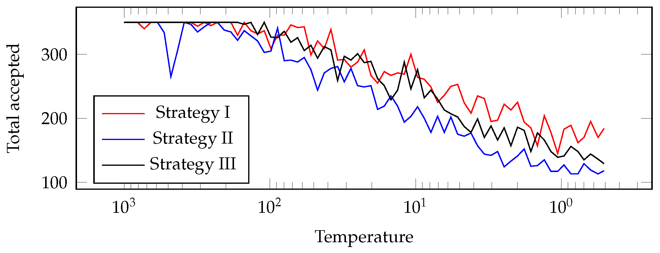
IV	$c_k\leftarrow 1$	$c_k\leftarrow c_k-3$	$c_k\leftarrow c_k+1$

shows three examples of feedback strategies, and additional strategies can be proposed. According to our experience, the negative feedback is always the same: the crystallization factor is incremented by 1.

Strategy I resets the crystallization factor $c_k$ to the unit. This strategy must be used when the objective function requires more exploration. The algorithm can generate a $x^{*}$ using larger jumps with higher probability. For example, the global optimum of an objective function with several local minima can be found using this strategy. Strategy III decrements the crystallization factor $c_k$ by one unit. This strategy must be used when the objective function requires more refinement. The algorithm generates smaller jumps when generating $x^{*}$.

Strategy II stays between strategies I and III. In this strategy, the crystallization factor is divided by 2. Strategy IV is a hybrid strategy in which the value attributed to the crystallization factor $c_k$ depends on the algorithm phase: the exploratory or refinement phase. Tavares et al. explained that the objective function standard deviation can determine the transition temperature when the algorithm goes from the exploratory to refinement phase [23]. The hybrid strategy performs exploration during the exploratory phase and performs refinement during the refinement phase. All four proposed strategies are used in this research. In the benchmark tests, strategies I and IV are used. The EIT application uses strategy II, and the airplane design application uses strategies I, II, and III.

2.3. Additional Settings

The initial temperature is an important parameter. The determination of the appropriate temperature is not a difficult task. It is recommended to fix a temperature that is high enough to ensure that SA is in the exploratory phase. If the temperature is high enough, the percentage of accepted candidates is 100%. Under this condition, SA performs only a random search and accepts everything. As the temperature decreases and reaches $80\%$ of accepted candidates, this is the appropriate initial temperature. Alternative approaches for the determination of the initial temperature exist in the literature [24].

The cooling schedule also is relevant for convergence [25]. Several proposals exist in the literature; a good review can be found in [23]. The EIT and airplane design applications use $\alpha =0.98$. For the benchmark tests, the adaptive cooling schedule explained in [23] is used. In this case, $\alpha$ is determined for each temperature and depends on the objective function’s standard deviation during the specific temperature.

The SA is terminated when the global condition is reached. The global condition represents the frozen state—it is a temperature where no candidate is accepted. In the EIT and airplane design applications, a small percentage of accepted solutions are used instead (such as $1\%$). In the benchmark tests, the algorithm is terminated when the number of objective function evaluations is reached.

The second loop is terminated when the thermal equilibrium is reached at a specific temperature. The thermal equilibrium depends on the number of variables, which is considered N. For a specific temperature, the thermal equilibrium is reached when the objective function is evaluated $5N$ times or the number of accepted candidates reaches $2.5N$. The number of accepted candidates is half the number of evaluated objective functions. For some applications, it is possible for the number of objective function evaluations to be greater than $5N$.

The value of $\Delta r_k$ can be easily fixed considering the variable boundaries, and it is defined by

$$\Delta r_k=\frac{x_{k,max}-x_{k,min}}{4}$$

(4)

where $[x_{k,min},x_{k,max}]$ are the boundaries for variable k. Finally, $c_{max}$ is defined as equal to 20.

3. Benchmark Results

SA with the crystallization heuristic was applied to some benchmark functions.

Table 2. Definition of the benchmark functions.

Function	$\mathit{f}\left(\mathbf{X}\right)$
Sphere	${\sum }_{i=1}^n{x}_i^2$
Rosenbrock	${\sum }_{i=1}^{n-1}\left[100{(x_i^2-x_{i+1})}^2+{(1-x_i)}^2\right]$
Rastrigin	$10n+{\sum }_{i=1}^n(x_i^2-10cos\left(2\pi x_i\right))$
Griewangk	$1+\frac{1}{4000}{\sum }_{i=1}^n{x}_i^2-{\prod }_{i=1}^{n}cos\left(\frac{x_i}{\sqrt{i}}\right)$
Ackley	$20-exp\left(\frac{1}{n}{\sum }_{i=1}^{n}cos\left(2\pi x_i\right)\right)+e-20exp\left(-0.2\sqrt{\frac{1}{n}{\sum }_{i=1}^n{x}_i^2}\right)$
Weierstrass	${\sum }_{i=1}^n\left[{\sum }_{j=0}^{20}\left[0.5^{j}cos\left(2\pi 3^j(x_i+0.5)\right)\right]\right]-n{\sum }_{j=0}^{20}\left[0.5^{j}cos\left(\pi 3^j\right)\right]$
Zakharov	${\sum }_{i=1}^n{x}_i^2+{\left({\sum }_{i=1}^n\frac{i}{2}{x}_i\right)}^2+{\left({\sum }_{i=1}^n\frac{i}{2}{x}_i\right)}^4$

shows the function definitions, with n being the number of variables.

Table 3. Limits and global optima of the benchmark functions.

Function	Limit	Global Optimum
Sphere	${[-100,100]}^n$	$f(0,\cdots ,0)=0$
Rosenbrock	${[-30,30]}^n$	$f(1,\cdots ,1)=0$
Rastrigin	${[-100,100]}^n$	$f(0,\cdots ,0)=0$
Griewangk	${[-600,600]}^n$	$f(0,\cdots ,0)=0$
Ackley	${[-40,40]}^n$	$f(0,\cdots ,0)=0$
Weierstrass	${[-10,10]}^n$	$f(0,\cdots ,0)=0$
Zakharov	${[-10,10]}^n$	$f(0,\cdots ,0)=0$

shows all the function limits and global optima. Each function has a different feature that is evaluated in this benchmark. The sphere function is the easiest function, with a global optimum that is well defined. The Rosenbrock function has a great deal of difficulty finding the global optimum once it is located in a flat-shaped valley. The Rastrigin, Ackley, Griewangk, and Weierstrass functions have several local minima, in which the capacity of the algorithm to escape these points is tested. The Zakharov function has a global optimum in place with a low gradient, making it difficult to determine with algorithms that use the gradient. Figure 3 shows all the functions plotted in a two-dimensional form; i.e., all functions have two variables.

All these functions are minimized with the proposed SA with the crystallization heuristic using two different positive feedback strategies: I and IV. The positive feedback strategy I resets the crystallization factor ($c_k\leftarrow 1$) every time a candidate is accepted (see Table 1). The positive feedback strategy IV resets the crystallization during the exploration phase and decreases the crystallization factor by three in the refinement phase every time a candidate is accepted. The verification of whether the algorithm is at an exploration or refinement phase is done by evaluating the standard deviation of the costs.

Each function is tested with three different numbers of variables: 10, 30, and 50. The maximum number of iterations is 10,000 times the number of variables. Each configuration is repeated 100 times, and the average and standard deviation of the cost are shown in

Table 4. Results of the benchmark function for 100 repetitions. N var is the number of variables, avg is the average of the costs, and std is the standard deviation. Strategy I is the reset of the crystallization factor, strategy IV is the hybrid decrease, reset of the crystallization in the beginning, and decrease by three unities at the end. According to Ingber, Matlab uses ASA [17,26]. PAGMO uses the SA approach proposed by Corana et al. [15,27]. The best results are emphasized in bold.

Function	N Var	Strategy I		Strategy IV		ASA-Matlab		SA-PAGMO
		Avg	Std	Avg	Std	Avg	Std	Avg	Std
Sphere	10	1.94 × 10${}^{-12}$	1.27 × 10${}^{-12}$	4.44 × 10${}^{-\mathbf{28}}$	1.39 × 10${}^{-\mathbf{28}}$	1.62 × 10${}^{-01}$	6.58 × 10${}^{-02}$	8.93 × 10${}^{-06}$	2.47 × 10${}^{-06}$
	30	6.23 × 10${}^{-12}$	2.46 × 10${}^{-12}$	2.69 × 10${}^{-\mathbf{27}}$	4.35 × 10${}^{-\mathbf{28}}$	3.69 × 10${}^{+00}$	5.31 × 10${}^{-01}$	7.06 × 10${}^{-05}$	1.05 × 10${}^{-05}$
	50	1.15 × 10${}^{-11}$	3.38 × 10${}^{-12}$	5.20 × 10${}^{-\mathbf{27}}$	6.53 × 10${}^{-\mathbf{28}}$	9.25 × 10${}^{+00}$	1.22 × 10${}^{+00}$	1.49 × 10${}^{-04}$	1.70 × 10${}^{-05}$
Rosenbrock	10	7.68 × 10${}^{-01}$	7.03 × 10${}^{-01}$	1.61 × 10${}^{-\mathbf{04}}$	2.87 × 10${}^{-\mathbf{04}}$	1.72 × 10${}^{+01}$	7.61 × 10${}^{+01}$	9.85 × 10${}^{-01}$	1.72 × 10${}^{+00}$
	30	3.43 × 10${}^{+01}$	3.32 × 10${}^{+01}$	9.97 × 10${}^{+00}$	2.34 × 10${}^{+01}$	1.63 × 10${}^{+01}$	1.16 × 10${}^{+01}$	5.59 × 10${}^{-\mathbf{01}}$	1.32 × 10${}^{+\mathbf{00}}$
	50	7.26 × 10${}^{+01}$	2.94 × 10${}^{+01}$	3.73 × 10${}^{+01}$	3.30 × 10${}^{+01}$	4.09 × 10${}^{+01}$	2.89 × 10${}^{+01}$	9.50 × 10${}^{+\mathbf{00}}$	6.06 × 10${}^{+\mathbf{00}}$
Rastrigin	10	1.58 × 10${}^{-07}$	7.24 × 10${}^{-08}$	0.00 × 10${}^{+\mathbf{00}}$	0.00 × 10${}^{+\mathbf{00}}$	4.39 × 10${}^{+01}$	1.81 × 10${}^{+01}$	1.69 × 10${}^{+01}$	5.62 × 10${}^{+00}$
	30	6.21 × 10${}^{-07}$	1.82 × 10${}^{-07}$	0.00 × 10${}^{+\mathbf{00}}$	0.00 × 10${}^{+\mathbf{00}}$	4.88 × 10${}^{+02}$	1.20 × 10${}^{+02}$	6.13 × 10${}^{+01}$	1.39 × 10${}^{+01}$
	50	1.09 × 10${}^{-06}$	2.51 × 10${}^{-07}$	0.00 × 10${}^{+\mathbf{00}}$	0.00 × 10${}^{+\mathbf{00}}$	1.31 × 10${}^{+03}$	2.24 × 10${}^{+02}$	1.04 × 10${}^{+02}$	1.92 × 10${}^{+01}$
Griewangk	10	7.13 × 10${}^{-\mathbf{02}}$	2.29 × 10${}^{-\mathbf{02}}$	7.86 × 10${}^{-02}$	3.16 × 10${}^{-02}$	1.26 × 10${}^{+00}$	1.38 × 10${}^{-01}$	2.81 × 10${}^{-01}$	1.28 × 10${}^{-01}$
	30	1.44 × 10${}^{-\mathbf{02}}$	1.61 × 10${}^{-\mathbf{02}}$	1.88 × 10${}^{-02}$	1.76 × 10${}^{-02}$	5.40 × 10${}^{+00}$	7.42 × 10${}^{-01}$	2.60 × 10${}^{-02}$	2.30 × 10${}^{-02}$
	50	7.36 × 10${}^{-\mathbf{03}}$	8.27 × 10${}^{-\mathbf{03}}$	1.11 × 10${}^{-02}$	1.77 × 10${}^{-02}$	1.19 × 10${}^{+01}$	1.35 × 10${}^{+00}$	1.19 × 10${}^{-02}$	1.36 × 10${}^{-02}$
Ackley	10	4.58 × 10${}^{-07}$	1.77 × 10${}^{-07}$	3.55 × 10${}^{-\mathbf{15}}$	0.00 × 10${}^{+\mathbf{00}}$	1.56 × 10${}^{+01}$	1.41 × 10${}^{+00}$	4.15 × 10${}^{-05}$	6.67 × 10${}^{-06}$
	30	8.29 × 10${}^{-07}$	1.89 × 10${}^{-07}$	9.24 × 10${}^{-\mathbf{15}}$	3.23 × 10${}^{-\mathbf{15}}$	2.03 × 10${}^{+01}$	1.67 × 10${}^{-01}$	2.03 × 10${}^{-04}$	1.93 × 10${}^{-05}$
	50	9.81 × 10${}^{-07}$	1.76 × 10${}^{-07}$	1.88 × 10${}^{-\mathbf{14}}$	3.41 × 10${}^{-\mathbf{15}}$	2.07 × 10${}^{+01}$	9.17 × 10${}^{-02}$	3.92 × 10${}^{-04}$	3.40 × 10${}^{-05}$
Weierstrass	10	4.38 × 10${}^{-04}$	1.17 × 10${}^{-04}$	0.00 × 10${}^{+\mathbf{00}}$	0.00 × 10${}^{+\mathbf{00}}$	3.96 × 10${}^{+00}$	7.27 × 10${}^{-01}$	1.51 × 10${}^{-02}$	1.49 × 10${}^{-01}$
	30	1.43 × 10${}^{-03}$	2.26 × 10${}^{-04}$	0.00 × 10${}^{+\mathbf{00}}$	0.00 × 10${}^{+\mathbf{00}}$	2.96 × 10${}^{+01}$	1.21 × 10${}^{+00}$	3.03 × 10${}^{-02}$	2.10 × 10${}^{-01}$
	50	2.42 × 10${}^{-03}$	2.59 × 10${}^{-04}$	0.00 × 10${}^{+\mathbf{00}}$	0.00 × 10${}^{+\mathbf{00}}$	5.88 × 10${}^{+01}$	2.73 × 10${}^{+00}$	3.06 × 10${}^{-02}$	2.10 × 10${}^{-01}$
Zakharov	10	4.58 × 10${}^{-07}$	3.64 × 10${}^{-07}$	6.02 × 10${}^{-\mathbf{17}}$	2.51 × 10${}^{-\mathbf{17}}$	2.51 × 10${}^{-01}$	9.57 × 10${}^{-02}$	1.06 × 10${}^{-05}$	3.43 × 10${}^{-06}$
	30	5.20 × 10${}^{+00}$	2.31 × 10${}^{+00}$	6.71 × 10${}^{-\mathbf{05}}$	6.94 × 10${}^{-05}$	2.39 × 10${}^{+00}$	5.20 × 10${}^{-01}$	1.24 × 10${}^{-04}$	3.43 × 10${}^{-\mathbf{05}}$
	50	1.21 × 10${}^{+02}$	2.48 × 10${}^{+01}$	1.59 × 10${}^{+00}$	6.40 × 10${}^{-\mathbf{01}}$	4.90 × 10${}^{+00}$	8.76 × 10${}^{-01}$	1.20 × 10${}^{+\mathbf{00}}$	1.34 × 10${}^{+00}$

. Strategy I is the positive feedback which resets the crystallization factor, and Strategy IV is the positive feedback strategy with a different strategy for the exploratory and refinement phase of the algorithm. The results show that the higher the number of variables, the worse the SA performs for both feedback strategies. Strategy IV performs better than Strategy I for all functions. This was expected, as every time the crystallization factor is restarted, it is necessary for several iterations to increase it to the point a new candidate is accepted. Then, the crystallization factor is kept low, making it difficult to refine to a better solution. The optimization performed by strategy I can achieve the results of strategy IV; however, a higher number of iterations will be necessary, making this strategy slower.

The proposed SA approach performed better in the Rastrigin and Weierstrass functions, finding the exact global minimum. The Sphere and Ackley functions had an average performance, followed by the Griewangk function. The Rosenbrock and Zakharov functions had the worst performance, especially in the tests with 50 variables (the source code used here to evaluate the proposed method is available at https://github.com/LabGeocomp/sacryst, 1 November 2021).

Table 4 also shows the results obtained using the Matlab and PAGMO SA algorithms. Matlab uses a SA approach based on ASA proposed by Ingber [17] and PAGMO (https://esa.github.io/pagmo2/docs/cpp/algorithms/simulated_annealing.html, 1 November 2021) uses a SA approach based on Corana et al.’s proposal [15,27]. The termination condition was a fixed number of objective function evaluations. The SA approach from PAGMO achieved the three best results: Rosenbrock with 30 and 50 variables, and Zakharov with 30 and 50 variables. As explained before, ASA uses the gradient information, which was not useful in this benchmark test.

4. SA with Incomplete Cost Evaluation Applied to EIT

EIT is a noninvasive imaging modality that provides safe medical imaging through a non-ionizing method. This technique converts its internal electrical conductivity distribution into a grayscale value, defining an image. Assuming there is no access to the interior of the body, the conductivity distribution must be inferred from electrical potential measurements taken on the surface of the body [28].

Several medical applications use EIT, which include the continuous observation of pulmonary function to assess the effects of therapeutic maneuvers on the regional distribution of ventilation [29,30], as well as monitoring cardiac activity [31]. Several nonclinical applications also use EIT, such as crack detection on mechanical components, detection of minerals in the soil, soil pollution monitoring, the visualization of multiphase flow, and real-time monitoring of industrial processes [32,33].

The EIT reconstruction problem can be solved by minimizing the difference between the observed data and a simulated impedance problem. The use of objective function derivatives is not recommended, as the EIT reconstruction is a nonlinear, nonconvex, and often ill-posed optimization problem. The objective function requires the solution of several Finite Element Method (FEM) problems, making it very computationally expensive. This work proposes a new SA approach in which the objective function is partially evaluated, while ensuring the boundaries of the proposed algorithm [34]. SA with an incomplete cost evaluation applied to EIT considers that the objective function returns an interval and a value. The value is an estimate of the precise objective function value and the interval contains the precise objective function value. It is shown below that the acceptance and rejection decision is not as simple as shown in Algorithm 2.

4.1. Equipment Configuration

A typical EIT configuration comprises the placement of electrodes along the contour of the object to be imaged. Then, a current of low amplitude is applied through an electrode pair, and the resulting electric potentials are measured at all electrodes. This process is repeated n times, applying the current across n different pairs of electrodes and taking electrical potential measurements. Figure 4 shows a 16-electrode EIT configuration for two current patterns: $J_1$ and $J_{13}$. The ensemble of measured potentials is denoted by $V=\{{\mathsf{\Phi }}_m^1,\cdots ,{\mathsf{\Phi }}_m^n\}$, where n is the number of current patterns and m is the number of electrodes [35].

4.2. Formulation of the Forward Problem

The EIT forward problem consists of calculating the potential distribution $\varphi$ within a domain $\mathsf{\Omega }$ given a conductivity distribution $\sigma$ and given an applied current pattern J. Since the frequencies of the applied current are low, the capacitive and inductive effects can be ignored, and so the 2D EIT problem satisfies the Laplace equation,

$$\nabla ·\left[\sigma \right(x,y)·\nabla \varphi (x,y\left)\right]=0,(x,y)\in \mathsf{\Omega },$$

(5)

where $\sigma$ and $\varphi$ are the conductivity and potential distributions, respectively, and $\mathsf{\Omega }$ is the domain. The equation is set to zero because there are no current sources inside the domain [36].

Solving the forward EIT problem consists of solving the Laplace equation in its weak form for $\varphi$, given the conductivity distribution $\sigma$ and the injected current J. The FEM is widely used to model forward problems, given its ability to model arbitrary geometry and boundary conditions [37,38]. In this case, the formulation of the forward problem of EIT by the FEM reduces the problem to the resolution of a linear system

$$K·\mathsf{\Phi }=J,$$

(6)

where J is the vector of injected currents, $\mathsf{\Phi }$ is the vector of potentials, and $K\in {\mathbb{R}}^{t\times t}$ is the conductance matrix [39].

4.3. The Inverse Problem

Reconstructing the conductivity distribution is an inverse problem. A valid solution would be a conductivity distribution that produces a given set of electric potential measurements. The EIT reconstruction problem can be solved by minimizing the difference between a simulated impedance domain and the one implied by the measured electric potential [40]. This is solved using SA to optimize the simulated impedance domain, using FEM to evaluate the solution at each iteration of the SA algorithm.

This optimization problem is in general strongly ill-conditioned and often nonconvex. Gradient-based optimization methods can converge to local minima and require special regularization terms to converge properly, which lead to the loss of detail in the reconstructed image.

A maximum a posteriori (MAP) probability estimate for the conductivity distribution based on Bayes’ rule can be performed using the measurements taken on the surface of the body, as well as the error estimates at each optimization iteration and some prior information of the expected conductivity distribution.

A MAP probability estimate of the conductivity distribution is one that maximizes

$$\pi \left(\sigma \right|V)\propto \pi \left(\sigma \right)\prod _{i=1}^n\chi ({\mathsf{\Phi }}_m^i-{\mathsf{\Phi }}_e^i)$$

(7)

where $\pi \left(\sigma \right)$ is a prior distribution for $\sigma$ and $\chi ({\mathsf{\Phi }}_m^i-{\mathsf{\Phi }}_e^i)$ is the probability density function (PDF) for a random error vector e, $\chi \left(e\right)=\chi ({\mathsf{\Phi }}_m^i-{\mathsf{\Phi }}_e^i)$, and ${\mathsf{\Phi }}_e^i$ is the vector of expected potentials at the electrodes. The optimization problem

$$\hat{\sigma }=argminE\left(\sigma \right)$$

(8)

is used to obtain a MAP estimation, where

$$E\left(\sigma \right)=\sum _{i=1}^n{\parallel {\mathsf{\Phi }}_m^i-{\mathsf{\Phi }}_e^i\parallel }^2+R\left(\sigma \right),$$

(9)

and $R\left(\sigma \right)\propto ln\left(\pi \right(\sigma \left)\right)$ is the regularization term, related to the prior knowledge of $\sigma$. Since the EIT problem is generally ill-posed, reconstruction is often impossible without prior knowledge [41].

4.4. Partial Evaluation and Interval SA

Evaluating the objective function on (9) typically requires solving a linear system. Since SA requires a large number of objective function evaluations, the total computational cost of a full EIT reconstruction by SA can become quite large. Let us suppose that it is possible to obtain an estimate for the objective functions $\tilde{E}$ bounded by upper and lower limits $E^{max}$ and $E^{min}$. Then, it is possible to obtain similar estimates for the variation of the objective function at the i-th iteration:

$$\begin{array}{cc}\hfill \Delta {\tilde{E}}_i& ={\tilde{E}}_i-{\tilde{E}}_{i-1}\hfill \\ \hfill \Delta E_i^{max}& =E_i^{max}-E_{i-1}^{min}\hfill \\ \hfill \Delta E_i^{min}& =E_i^{min}-E_{i-1}^{max}.\hfill \end{array}$$

This corresponds to the classical difference operation in interval arithmetic. Then, by the definition of the SA algorithm, if in a given iteration $\Delta \tilde{E}$, $\Delta E^{max}$, $\Delta E^{min}$ satisfy

$$exp(-\Delta E^{max}/T)\ge \left\{\begin{array}{cc}1-P_{\mathrm{err}}\hfill & if\Delta \tilde{E}\le 0,\hfill \\ exp(-\Delta \tilde{E}/T)-P_{\mathrm{err}}\hfill & if\Delta \tilde{E}>0\hfill \end{array}\right.$$

(10)

$$exp(-\Delta E^{min}/T)\le min(1,P_{\mathrm{err}}+exp(-\Delta \tilde{E}/T))$$

(11)

then an algorithm that uses the approximations ${\tilde{E}}_i$ has a probability of less than $P_{\mathrm{err}}$ of deviating from an algorithm that uses the exact values $E_i$.

In [32], this property is used by Martins and Tsuzuki to create stopping criteria for the underlying linear solvers that evaluate (9) for EIT reconstruction. By limiting the probability of deviation to less than $5\%$, EIT images were reconstructed by SA in as few as 20 iterations of a conjugated gradient solver operating on meshes of more than 1000 nodes.

4.5. Results and Discussion

The electrical potential measurements were taken from two different impedance distributions. Figure 5 displays the two distributions, which consisted of placing three phantoms made of cucumber slices in random positions inside of a saline solution. The reconstructed images are shown in Figure 6 for the two configurations. The saline water has almost constant conductivity. The cucumbers are visible according to the established arrangement. These results have a good contrast, determining the boundaries of the internal elements. When compared with the results of other approaches, these results show an improvement in the internal element boundaries determination [30,42].

Figure 7 shows the convergence of SA with the crystallization factor for both arrangements; the two graphs are shown in blue. Averagely, larger values of the cost function show that the exploration phase is happening at higher temperatures. The graph shows that the exploration phase is very short for both arrangements. At lower temperatures, lower values of the cost function on average show that the refinement phase happens. Martins and Tsuzuki [43] showed that the application of interval SA with the crystallization factor to EIT created an emergent behavior: external layers converged first and internal layers converged later. The possibility of convergence layer by layer was first proposed by Somersalo et al. [44]. However, it was shown to be unstable in the presence of noise. The algorithm proposed by Martins and Tsuzuki [43] is the first stable implementation with this property [45]. Tavares et al. [46] developed a new heuristic, called outside-in, using this emergent behavior.

In the two graphs in red shown in Figure 7, the number of conjugated gradient iterations is represented on average for each temperature. The mesh used in the reconstruction has more than 1000 nodes. Consequently, the linear system (6) has more than 1000 equations, and the number of iterations that the conjugated gradient must perform is the same as the number of equations. Considering Figure 7, the maximum number of conjugated gradient iterations is 35. As the cost function is partially evaluated, the number of conjugated iterations is kept at a small number.

The number of conjugated gradient iterations at higher temperatures is smaller when compared to the iterations at lower temperatures. As previously pointed, the cost function is partially evaluated and, simultaneously, the interval $\Delta E_i=\left[E_i^{min},E_i^{max}\right]$ in which the exact value is contained is also determined. At higher temperatures, SA performs exploration and the determined $\Delta E_i$ is larger. Usually, the candidates are far from the final solution and larger errors are present. At lower temperatures, SA performs refinement, and the determined $\Delta E_i$ must be small. The number of conjugated gradient iterations is kept at a reasonable level (smaller than 35 iterations) because the initial linear system solution for the conjugated gradient current is the final linear system solution from the previous conjugated gradient evaluation. Considering that only a small modification happens, remember that only one parameter is modified at a time, as shown in Algorithm 2; the final linear system solution from the previous conjugated gradient evaluation is a good initial linear system solution for the current conjugated gradient evaluation.

Table 5. Results of tests for the two arrangements. The final cost and the total number of cost function evaluations.

Arrangement	Cost	Total Iteration
Linear arrangement	28.02	1,876,819
Triangular arrangement	19.71	1,930,430

shows the final cost and the number of cost function evaluations for the two experimental arrangements. Occasionally, the linear arrangement converges first with a smaller number of cost function evaluations. The SA has aleatory convergence, and the final cost and the total number of cost function evaluations can change. However, the reconstructed image for the two arrangements is always very similar, showing that the proposed interval SA with partial evaluation of the cost function is robust. A similar algorithm was also applied to the anisotropic domain [34].

5. SA Applied to Aircraft Design

The proposed SA approach can be used for various engineering design problems. Considering the nature of any engineering design problem, it is important to have a systematic method in place to control the sequence of design tasks and define the work transfer among various design stages [47]. The work transfer requirement will also be used to define the objective functions and the corresponding optimization parameters. Examples of these structured design procedures can be seen in the design of the handling mechanism in a racing car [48], with the design of curved structures for optimum vibrational properties [49]. Various engineering requirements including the consideration of manufacturing limitations can be introduced to the problem as optimization constraints [50,51]. The SAE organizes an annual Aero Design competition in which engineering students are challenged to design and manufacture a radio-controlled aircraft [52]. The main goal of this competition is to develop the lightest aircraft that lifts the largest possible load. Designs are required to follow a set of constraints such as a maximum allowable dimensional sum, specific motor and manufacturing materials, and runway length.

The score is determined through a list of factors such as reliability (an accepted accuracy curve shows the maximum payload given the temperature and pressure statistics), total load (the sum of the aircraft weight and payload), and structural efficiency (ratio between payload and self-weight). During the conceptual design phase, participants define significant characteristics of their design. However, it is very difficult to determine a possible geometric design in the initial phase due to the large number of possible configurations. This work uses SA with the crystallization heuristic to search for the aircraft geometry that would have the highest score. Aircraft geometry is parameterized according to the the design characteristics and subsequently optimized to carry the largest load while being as light as possible and following the rules of the competition.

5.1. Aircraft Design Evaluation Process

Applying SA to the optimization of aircraft design requires a method for evaluating prospective designs that can be applied at each iteration of the algorithm [53]. In this case, the design must be validated according to the competition rules and a given score. The competition outlines several constraints for the design, and a violation of any one of these constraints invalidates it. As such, only designs that meet all the requirements can be given a score. The constraints are checked in the order outlined in Figure 8 and are described as follows:

• Dimensional constraint: The sum of the height, width, and length must be below the upper limit;
• Aerodynamic evaluation: This depends on the wing and tail geometry;
• Stability evaluation: The approximate weight of the aircraft is determined using the material density and the volume of the stringer;
• Motor placement: The motor must be more than 8 cm from the fuselage;
• Structural evaluation: All mechanical stresses are evaluated.

Once the design is validated, it is given a score based on its maximum load, which is estimated from the geometry and the runway length as set by the regulations.

The design must also be parameterized for the algorithm to be applicable. The para metrization scheme consists of 23 parameters (19 continuous variables and 4 discrete variables). Such parametrization is sufficient to calculate the aerodynamic coefficients in the aerodynamic evaluation as well as to estimate the score.

5.2. Results and Discussion

SA with crystallization heuristics was used to optimize three aircraft designs with three different positive feedback strategies: I, II, and III (see Table 1). Strategy I performs the positive feedback with a small decrement, focusing on refining the solution. However, if SA stays in a local minima at lower temperature, it will be very difficult to escape from it. Strategy III focuses on exploring the solution space, allowing an easy escape from local minima. Strategy II has a balance between refinement and exploration. The crystallization factor evolution, the acceptance and rejection ratios, as well as the best aircraft for each feedback strategy are shown with respect to the five parameters.

Through the optimization process, five parameters showed the largest variations: AA (projected superior area of the wing), DHBA (horizontal distance between leading edges), CF (fuselage chord), A1 (percentage of wingspan designated to Section 1), and TS1 (taper ratio of Section 1). Figure 9 shows a representation of an aircraft and these five parameters. Notice that the yellow region of the wing is defined as Section 1, and the blue region is defined as Section 2.

Figure 10 shows the crystallization factor evolution for each positive feedback strategy. Figure 10a shows the expected behavior for the crystallization factors. At higher temperatures, the crystallization factor is small and SA performs exploration. The crystallization factor grows gradually; at lower temperatures, SA performs refinement. However, each parameter might have different sensibilities and, consequently, different crystallization factors. Figure 10b shows the positive feedback strategy II, and the crystallization factors of parameters TS1 and CF do not increase as much as the other three parameters. When compared to strategy I, these two parameters stay in an exploratory phase during the complete algorithm. Figure 10c shows the positive feedback strategy III and shows a considerable variation at the end of the refinement phase. Notice the difference between the crystallization factors: while the positive feedback strategies I and III reached higher values at the end of convergence (more than 600 in the first method), the positive feedback strategy II barely reached 150.

Figure 11 shows the acceptance ratio for each positive feedback strategy—the acceptance ratio is the ratio between the number of accepted candidates and the total number of candidates. If the ratio is equal to $1.0$, this means that all candidates were accepted. The ratio is calculated separately for each parameter. As previously shown, it is necessary to increase the number of accepted candidates as much as possible. Usually, the acceptance ratio decreases with the temperature. SA reaches a frozen state when no new candidate is accepted. There is a difference between the positive feedback strategies at lower temperatures. Figure 11a shows a small variation of the acceptance ratios at lower temperatures. Figure 11b shows the smallest acceptance ratio among the three positive feedback strategies. Figure 11c shows a large variation in the acceptance ratios. Each parameter might have its own appropriate positive feedback strategy.

Figure 12 shows the total number of accepted solutions. As expected, the number of accepted solutions decreases as the temperature decreases. It is not possible to observe differences between the positive feedback strategies. Figure 13 shows the population dispersion for each positive feedback strategy considering only two intermediary parameters: (1) dimensional sum and (2) payload. The dimensional sum is the summation of the three maximum dimensions in the three axes x, y, and z. The dimensional sum has an associated design constraint: the “dimensional constraint”. It cannot be larger than a specific value defined by the competition. By observing the graphs, it can be seen that the larger the dimensional sum, the higher the payload. Figure 13a shows the largest concentration of solutions at the higher payload. Figure 13b shows an intermediary exploration. Figure 13c a higher exploration of the full domain. One possible heuristic that can be deduced from these results is to always keep the maximum dimensional sum.

The x and y dimensions can be freely decided, but the z dimension is determined based on a new rule. The z dimension must be the maximum dimensional sum reduced by the x and y dimensions. Using this empirical rule, the optimization will search in a domain with higher scores, and this will be faster (as one constraint is always satisfied by construction).

Figure 14 shows the best aircraft for each positive feedback strategy. The aircrafts from positive feedback strategies I and III are similar, while the aircraft from positive feedback II is different than the others. It can be seen that strategies I and II reached the highest scores and strategies I and III reached similar designs.

6. Conclusions

This paper discusses the advantages and significance of using the SA algorithm with the crystallization heuristic to solve different problems. The crystallization heuristic represents the sensibility of parameters represented by a real number. The crystallization heuristic ensures the escape from local minima even at lower temperatures. This is a key factor for solving highly nonlinear objective functions that can be seen in many engineering design and manufacturing problems. The proposed SA with crystallization approach was applied to several benchmark problems from the literature, characterizing its performance. SA has two main phases of exploration and refinement. Different strategies for implementing the positive feedback are shown, and their connection with the two SA phases is also displayed. Exploration even at lower temperatures is emphasized as a strategy. Two engineering designs have been addressed in this paper as case studies that can be solved properly using the proposed methodology. The first application case study presented the design of an Electrical Impedance Tomography system. This implemented the partial evaluation of the cost function, returning an interval in which the precise result was contained. The interval SA with crystallization heuristic approach converged with a smaller number of conjugated gradient iterations (only near 3% of the required iterations were performed). The second case study was part of an aircraft design, which resulted in an optimization with constraints.

References

1. Li, C.; Wang, X. Gauss-Newton methods for a class of nonsmooth optimization problems. Prog. Nat. Sci. 2000, 10, 472–473. [Google Scholar]
2. Etter, D.M.; Hicks, M.J.; Cho, K.H. Recursive adaptive filter design using an adaptive genetic algorithm. In Proceedings of the IEEE ICASSP, Paris, France, 3–5 May 1982; pp. 635–638. [Google Scholar]
3. Castro, E.G.; Tsuzuki, M.S.G. Swarm Intelligence applied in synthesis of hunting strategies in a three-dimensional environment. Expert Syst. Appl. 2008, 34, 1995–2003. [Google Scholar] [CrossRef]
4. Kirkpatrick, S. Optimization by simulated annealing: Quantitative studies. J. Stat. Phys. 1984, 34, 975–986. [Google Scholar] [CrossRef]
5. Hasegawa, A.Y.; Rosso, R.S.; Tsuzuki, M.S.G. Bézier Curve Fitting With A Parallel Differential Evolution Algorithm. IFAC Proc. Vol. 2013, 46, 233–238. [Google Scholar] [CrossRef]
6. Changdar, C.; Mahapatra, G.; Pal, R. A modified genetic algorithm-based approach to solve constrained solid TSP with time window using interval valued parameter. Int. J. Oper. Res. 2016, 26, 398–421. [Google Scholar] [CrossRef]
7. Vallade, B.; Nakashima, T. Improving particle swarm optimization algorithm and its application to physical travelling salesman problems with a dynamic search space. Stud. Comp. Intell. 2014, 553, 105–119. [Google Scholar]
8. Granville, V.; Krivanek, M.; Rasson, J.P. Simulated annealing: A proof of convergence. IEEE Trans. Pattern Anal. 1994, 16, 652–656. [Google Scholar] [CrossRef]
9. Goto, T.G.; Najafabadi, H.R.; Duran, G.C.; Ueda, E.K.; Sato, A.K.; Martins, T.C.; Takimoto, R.Y.; Gohari, H.; Barari, A.; Tsuzuki, M.S.G. Versatility of Simulated Annealing with Crystallization Heuristic: Its Application to a Great Assortment of Problems. In Optimization Problems in Engineering [Working Title]; IntechOpen: London, UK, 2021. [Google Scholar] [CrossRef]
10. Martins, T.C.; Tsuzuki, M.S.G. Simulated annealing applied to the rotational polygon packing. IFAC Proc. Vol. 2006, 39, 475–480. [Google Scholar] [CrossRef]
11. Martins, T.C.; Tsuzuki, M.S.G. Rotational placement of irregular polygons over containers with fixed dimensions using simulated annealing and no-fit polygons. J. Braz. Soc. Mech. Sci. 2008, 30, 205–212. [Google Scholar] [CrossRef] [Green Version]
12. Sato, A.K.; Martins, T.C.; Tsuzuki, M.S.G. Rotational Placement using Simulated Annealing and Collision Free Region. IFAC Proc. Vol. 2010, 43, 234–239. [Google Scholar] [CrossRef]
13. Metropolis, N.; Rosenbluth, A.W.; Rosenbluth, M.N.; Teller, A.H.; Teller, E. Equation of state calculations by fast computing machines. J. Chem. Phys. 1953, 21, 1087–1092. [Google Scholar] [CrossRef] [Green Version]
14. Kirkpatrick, S.; Gelatt, C.D.; Vecchi, M.P. Optimization by simulated annealing. Science 1983, 220, 671–680. [Google Scholar] [CrossRef]
15. Corana, A.; Marchesi, M.; Martini, C.; Ridella, S. Minimizing multimodal functions of continuous variables with the simulated annealing algorithm. ACM Trans. Math. Softw. 1987, 13, 262–280. [Google Scholar] [CrossRef]
16. Bohachevsky, I.O.; Johnson, M.E.; Stein, M.L. Generalized simulated annealing for function optimization. Technometrics 1986, 28, 209. [Google Scholar] [CrossRef]
17. Ingber, L. Very fast simulated re-annealing. Math. Comput. Model. 1989, 12, 967–973. [Google Scholar] [CrossRef] [Green Version]
18. Tsuzuki, M.S.G.; Martins, T.C.; Takase, F.K. Robot path planning using simulated annealing. IFAC Proc. Vol. 2006, 39, 175–180. [Google Scholar] [CrossRef]
19. Martins, T.C.; Tsuzuki, M.S.G. Placement over containers with fixed dimensions solved with adaptive neighborhood simulated annealing. Bull. Pol. Acad. Sci. 2009, 57, 273–280. [Google Scholar] [CrossRef] [Green Version]
20. Bates, G.E. Joint distributions of time intervals for the occurrence of successive accidents in a generalized polya scheme. Ann. Math. Stat. 1955, 26, 705–720. [Google Scholar] [CrossRef]
21. Ueda, E.K.; Sato, A.K.; Martins, T.C.; Takimoto, R.Y.; Rosso, R.S.U., Jr.; Tsuzuki, M.S.G. Curve approximation by adaptive neighborhood simulated annealing and piecewise Bézier curves. Soft Comput. 2020, 24, 18821–18839. [Google Scholar] [CrossRef]
22. Ueda, E.K.; Tsuzuki, M.S.; Barari, A. Piecewise Bézier curve fitting of a point cloud boundary by simulated annealing. In Proceedings of the 13th IEEE INDUSCON, São Paulo, Brazil, 12–14 November 2018; pp. 1335–1340. [Google Scholar]
23. Tavares, R.S.; Martins, T.C.; Tsuzuki, M.S.G. Simulated annealing with adaptive neighborhood: A case study in off-line robot path planning. Expert Syst. Appl. 2011, 38, 2951–2965. [Google Scholar] [CrossRef]
24. Lee, C.Y. Fast simulated annealing with a multivariate Cauchy distribution and the configuration’s initial temperature. J. Korean Phys. Soc. 2015, 66, 1457–1466. [Google Scholar] [CrossRef]
25. Cohn, H.; Fielding, M. Simulated annealing: Searching for an optimal temperature schedule. SIAM J. Optim. 1999, 9, 779–802. [Google Scholar] [CrossRef]
26. Moins, S. Implementation of a Simulated Annealing Algorithm for Matlab Training Performed; Linköping University: Linköping, Sweden, 2002. [Google Scholar]
27. Simulated Annealing (Corana’s Version)—Pagmo 2.18.0 Documentation. Available online: https://esa.github.io/pagmo2/ (accessed on 8 November 2012).
28. Martins, T.C.; Tsuzuki, M.S.G.; Camargo, E.D.L.B.; Lima, R.G.; Moura, F.S.D.; Amato, M.B.P. Interval Simulated Annealing applied to Electrical Impedance Tomography image reconstruction with fast objective function evaluation. Comput. Math. Appl. 2016, 72, 1230–1243. [Google Scholar] [CrossRef]
29. Hua, P.; Woo, E.J.; Webster, J.G.; Tompkins, W.J. Finite element modeling of electrode-sking contact impedance in electrical impedance tomography. IEEE Trans. Biomed. Eng. 1993, 40, 335–343. [Google Scholar] [CrossRef]
30. Trigo, F.C.; Lima, R.G.; Amato, M.B.P. Electrical impedance tomography using the extended Kalman filter. IEEE Trans. Biomed. Eng. 2004, 51, 72–81. [Google Scholar] [CrossRef]
31. Eyüboglu, B.M.; Brown, B.H.; Barber, D.C. In vivo imaging of cardiac related impedance changes. IEEE Eng. Med. Biol. 1989, 8, 39–45. [Google Scholar] [CrossRef]
32. Martins, T.C.; Tsuzuki, M.S.G. Electrical impedance tomography reconstruction through simulated annealing with total least square error as objective function. In Proceedings of the 34th IEEE EMBC, San Diego, CA, USA, 28 August–1 September 2012; pp. 1518–1521. [Google Scholar]
33. Silva, O.L.; Lima, R.G.; Martins, T.C.; Moura, F.S.; Tavares, R.S.; Tsuzuki, M.S.G. Influence of current injection pattern and electric potential measurement strategies in electrical impedance tomography. Control Eng. Pract. 2017, 58, 276–286. [Google Scholar] [CrossRef]
34. Martins, T.C.; Tsuzuki, M.S.G. Investigating anisotropic EIT with simulated annealing. IFAC-PapersOnLine 2017, 50, 9961–9966. [Google Scholar] [CrossRef]
35. Tavares, R.S.; Nakadaira-Filho, F.A.; Tsuzuki, M.S.G.; Martins, T.C.; Lima, R.G. Discretization error and the EIT forward problem. IFAC-PapersOnLine 2014, 47, 7535–7540. [Google Scholar] [CrossRef]
36. Martins, T.C.; Fernandes, A.V.; Tsuzuki, M.S.G. Image reconstruction by electrical impedance tomography using multi-objective simulated annealing. In Proceedings of the 11th IEEE ISBI, Beijing, China, 28 April–2 May 2014; pp. 185–188. [Google Scholar]
37. Martins, T.C.; Tsuzuki, M.S.G. Electrical impedance tomography reconstruction through simulated annealing with multi-stage partially evaluated objective functions. In Proceedings of the 35th IEEE EMBC, Osaka, Japan, 3–7 July 2013; pp. 6425–6428. [Google Scholar]
38. Bianchessi, A.; Akamine, R.H.; Duran, G.C.; Tanabi, N.; Sato, A.K.; Martins, T.C.; Tsuzuki, M.S.G. Electrical impedance tomography image reconstruction based on neural networks. IFAC-PapersOnLine 2020, 53, 15946–15951. [Google Scholar] [CrossRef]
39. Martins, T.C.; Camargo, E.D.L.B.; Lima, R.G.; Amato, M.B.P.; Tsuzuki, M.S.G. Electrical impedance tomography reconstruction through simulated annealing with incomplete evaluation of the objective function. In Proceedings of the 33rd IEEE EMBC, Boston, MA, USA, 30 August–3 September 2011; pp. 7033–7036. [Google Scholar]
40. Tavares, R.S.; Sato, A.K.; Martins, T.C.; Lima, R.G.; Tsuzuki, M.S.G. GPU acceleration of absolute EIT image reconstruction using simulated annealing. Biomed. Signal Process. 2019, 52, 445–455. [Google Scholar] [CrossRef]
41. Martins, T.C.; Tsuzuki, M.S.G. EIT image regularization by a new multi-objective simulated annealing algorithm. In Proceedings of the 37th IEEE EMBC, Milan, Italy, 25–29 August 2015; pp. 4069–4072. [Google Scholar]
42. Martins, T.C.; Camargo, E.D.L.B.; Lima, R.G.; Amato, M.B.P.; Tsuzuki, M.S.G. Image reconstruction using interval simulated annealing in electrical impedance tomography. IEEE Trans. Biomed. Eng. 2012, 59, 1861–1870. [Google Scholar] [CrossRef]
43. Martins, T.C.; Tsuzuki, M.S.G. Simulated annealing with partial evaluation of objective function applied to electrical impedance tomography. IFAC Proc. Vol. 2011, 44, 4989–4994. [Google Scholar] [CrossRef] [Green Version]
44. Somersalo, E.; Cheney, M.; Isaacson, D.; Isaacson, E. Layer stripping: A direct numerical method for impedance imaging. Inverse Probl. 1991, 7, 899–926. [Google Scholar] [CrossRef]
45. Martins, T.C.; Sato, A.K.; Moura, F.S.; Camargo, E.D.L.B.; Silva, O.L.; Santos, T.B.R.; Zhao, Z.; Möeller, K.; Amato, M.B.P.; Mueller, J.L.; et al. A review of electrical impedance tomography in lung applications: Theory and algorithms for absolute images. Annu. Rev. Control 2019, 48, 442–471. [Google Scholar] [CrossRef] [PubMed]
46. Tavares, R.S.; Martins, T.C.; Tsuzuki, M.S.G. Electrical impedance tomography reconstruction through simulated annealing using a new outside-in heuristic and GPU parallelization. J. Phys. Conf. Ser. 2012, 407, 012015. [Google Scholar] [CrossRef] [Green Version]
47. Platanitis, G.; Pop-Iliev, R.; Barari, A. Development of a DSM-based methodology in an academic setting. J. Mech. Des. 2012, 134, 021007. [Google Scholar] [CrossRef]
48. Diba, F.; Barari, A.; Esmailzadeh, E. Handling and safety enhancement of race cars using active aerodynamic systems. Veh. Syst. Dyn. 2014, 52, 1171–1190. [Google Scholar] [CrossRef]
49. Askari, H.; Esmailzadeh, E.; Barari, A. A unified approach for nonlinear vibration analysis of curved structures using non-uniform rational B-Spline representation. J. Sound Vib. 2015, 353, 292–307. [Google Scholar] [CrossRef]
50. Barari, A.; ElMaraghy, H.A.; Orban, P. NURBS representation of estimated surfaces resulting from machining errors. Int. J. Comp. Integr. Manuf. 2009, 22, 395–410. [Google Scholar] [CrossRef]
51. Jankovics, D.; Barari, A. Customization of automotive structural components using additive manufacturing and topology optimization. IFAC-PapersOnLine 2019, 52, 212–217. [Google Scholar] [CrossRef]
52. Sato, A.K.; Borburema, D.M.; Tsuzuki, M.S.G.; Ueda, E.K.; Martins, T.C.; Mariani, A.L.C. Simulated annealing with crystallization heuristic applied to aircraft conceptual design. In Proceedings of the 11th IEEE INDUSCON, Juiz de Fora, Brazil, 7–10 December 2014. [Google Scholar]
53. Borburema, D.M.; Sato, A.K.; Tsuzuki, M.S.G. Design and optimization of UAV for surveillance at Fernando de Noronha’s risk areas. In Proceedings of the 13th IEEE INDUSCON, São Paulo, Brazil, 12–14 November 2019; pp. 413–418. [Google Scholar]
Figure 1. SA has two clear phases in the optimization process: exploration and refinement. The crystallization factors have a connection with the two phases. During the exploration phase, larger jumps are performed (the parameters have lower crystallization). During the refinement phase, the optimization performs smaller jumps with higher probability (the parameters have higher crystallization). Δ r k is fixed for each variable and represents the distribution width.
Applsci 11 11814 g001
Figure 2. SA provides a feedback to the crystallization factor associated with the modified variable. If the solution is accepted, the crystallization factor is reduced (positive feedback). If the solution is rejected, the crystallization factor is increased (negative feedback).
Applsci 11 11814 g002
Figure 3. Plot of the functions with two variables. (a) Sphere, (b) Rosenbrock, (c) Rastrigin, (d) Griewangk, (e) Ackley, (f) Weierstrass, (g) Zakharov.
Applsci 11 11814 g003
Figure 4. Given a domain with a conductivity distribution σ ( x , y ) , EIT equipment is used to measure the electrical potential Φ j i on all j [ 1 , 16 ] electrodes from the injection of the current pattern J i .
Applsci 11 11814 g004
Figure 5. Electrical potential measurements were taken for two conductivity distributions. (a) Physical linear arrangement. (b) Physical triangular arrangement.
Applsci 11 11814 g005
Figure 6. The reconstructed for the two conductivity distributions in ( Ω · m ) 1 . (a) Linear arrangement reconstructed. (b) Triangular arrangement reconstructed.
Applsci 11 11814 g006
Figure 7. The graphs in blue show the cost function average for each temperature. It represents the convergence of SA. The graphs show a short exploration phase and a longer refinement phase. The graphs in red show the number of conjugated gradient iterations on average for each temperature. (a) Linear arrangement. (b) Triangular arrangement.
Applsci 11 11814 g007
Figure 8. Flowchart of constraint verification. Starting from a candidate (the new configuration), different constraints are verified in sequence. If any constraint is not satisfied, a new candidate is selected.
Applsci 11 11814 g008
Figure 9. Schematic representation of the airplane. A set of parameters is shown: CF (fuselage chord), DHBA (horizontal distance between leading edges), and Section 1 (percentage of wingspan represented as A1, and tapper ration represented as TS1).
Applsci 11 11814 g009
Figure 10. Crystallization factor evolution according the three positive feedback strategies. (a) Enhancing the refinement. (b) Good balance between refinement and exploration. (c) Enhancing the exploration.
Applsci 11 11814 g010
Figure 11. The accepted solution ratio for each parameter is shown for all the three positive feedback strategies. (a) The refinement is enhanced. (b) There is a balance between refinement and exploration. (c) The exploration is enhanced.
Applsci 11 11814 g011
Figure 12. Total number of accepted solutions for each temperature.
Applsci 11 11814 g012
Figure 13. The influence of some intermediary parameters with the final score: the dimensional sum and payload. The score is represented in colors. (a) Strategy I, (b) Strategy II, (c) Strategy III.
Applsci 11 11814 g013
Figure 14. Best aircraft design obtained from each positive feedback strategy. (a) Strategy I, (b) Strategy II, (c) Strategy III.
Applsci 11 11814 g014